
MBNet: Multi-Branch Network for Extraction of Rural Homesteads Based on Aerial Images

1
Institute of Agricultural Information, Chinese Academy of Agricultural Sciences, Beijing 100081, China
2
Key Laboratory of Agricultural Blockchain Application, Ministry of Agriculture and Rural Affairs, Beijing 100125, China
*
Author to whom correspondence should be addressed.
Remote Sens. 2022, 14(10), 2443; https://0-doi-org.brum.beds.ac.uk/10.3390/rs14102443
Submission received: 2 April 2022
/
Revised: 12 May 2022
/
Accepted: 17 May 2022
/
Published: 19 May 2022
Abstract
:Deep convolution neural network (DCNN) technology has achieved great success in extracting buildings from aerial images. However, the current mainstream algorithms are not satisfactory in feature extraction and classification of homesteads, especially in complex rural scenarios. This study proposes a deep convolutional neural network for rural homestead extraction consisting of a detail branch, a semantic branch, and a boundary branch, namely Multi-Branch Network (MBNet). Meanwhile, a multi-task joint loss function is designed to constrain the consistency of bounds and masks with their respective labels. Specifically, MBNet guarantees the details of prediction through serial 4× down-sampled high-resolution feature maps and adds a mixed-scale spatial attention module at the tail of the semantic branch to obtain multi-scale affinity features. At the same time, the low-resolution semantic feature maps and interaction between high-resolution detail feature maps are maintained. Finally, the result of semantic segmentation is refined by the point-to-point module (PTPM) through the generated boundary. Experiments on UAV high-resolution imagery in rural areas show that our method achieves better performance than other state-of-the-art models, which helps to refine the extraction of rural homesteads. This study demonstrates that MBNet is a potential candidate for building an automatic rural homestead management system.

1. Introduction
As an essential division of China’s rural land, rural homesteads ensure the basic welfare of farmers and have been a worldwide focus. A comprehensive understanding of the fundamental information such as the scale, layout, ownership, and utilization status of homesteads can provide support for deepening the reform of the rural homestead system. The commonly used statistics of rural homestead-related information mainly depend on the traditional methods such as field surveys and surveying and mapping [1]. Since these methods suffer from a large workload, long cycle, and low efficiency, it is difficult to meet the country’s needs for homestead statistics and management [2]. In recent years, the development of high-resolution remote sensing image technology has provided new measures for obtaining homestead information. As a kind of remote sensing images, low-altitude unmanned aerial vehicle (UAV) images have a higher resolution than satellite images, which helps obtain large-scale and detailed information on the distribution of homesteads in rural areas without intensive labor. However, using manual visual interpretation alone to illustrate remotely sensed images will also involve great manpower and time costs, which poses serious challenges when addressing thousands of rural homestead surveys. Therefore, this requires fast and accurate automation technologies to interpret the rural homesteads in remote sensing images.
The essence of rural homestead recognition is to extract the rural buildings and related areas from the images. The use of high-resolution remote sensing images to automatically extract buildings has always been a hot issue, and it has great significance for urban and rural planning, map updating, disaster assessment, geographic information system database updating, and other applications [3,4,5]. With the development of deep learning technologies, fast and accurate building extraction has become possible. Due to the irregular shapes and boundaries of buildings, the semantic segmentation method appears to be the most prospective for precisely extracting buildings in high-resolution remote sensing images, and the extracted targets can also be used further for subsequent analysis and calculations. The contribution of the pioneering work of deep learning in the field of semantic segmentation, fully convolutional networks (FCNs), is to employ an end-to-end convolution neural network and also use deconvolution for up-sampling [6]. Furthermore, a jump connection method was used to fuse the deep and shallow information of the network. Then, U-Net added a channel feature fusion method on the basis of FCN, fusing the underlying information and advanced information in the channel dimension, which is more helpful for obtaining boundary information [7]. As the latest version of the DeepLab series proposed by Google, DeepLabV3+ employed the encoder–decoder architecture and atrous spatial pyramid pooling module to obtain multi-scale spatial information and integrate low-level features into high-level semantic information [8]. DANet combines channel attention mechanism and spatial attention mechanism to enhance the expression ability of foreground and make the network focus more on the target pixels [9]. Given that the semantic segmentation algorithms have achieved excellent performance, many scholars have improved the existing models suitable for urban building extraction. For instance, Xu et al. combined the attention mechanism module and the multi-scale nesting module to improve the U-Net algorithm [10]. Zhang et al. proposed the JointNet algorithm with atrous convolution to extract urban buildings and roads [11]. Ye et al. studied the semantic gap of features at different stages in semantic segmentation and re-weighted the attention mechanism to extract buildings [12]. Aiming at the problem of the difficulty of recognizing a building boundary using semantic segmentation, Xia et al. proposed the Dense D-LinkNet architecture to realize the precise extraction of the building [13].
Buildings in rural areas are generally scattered and disordered, but in partial areas, rural houses are closely connected. In order to calculate the quantitative indicators such as the number and area of rural homesteads, a high-precision algorithm is required to extract rural homesteads from satellite images. Recently, semantic segmentation methods have been successfully applied for extracting and detecting rural buildings. Pan et al. employed U-Net to extract and recognize urban village buildings based on Worldview satellite images [14]. Ye et al. combined Dilated-Resnet and SE-Module with FCN to discriminate rural settlements using Gaofen-2 images [15]. Sun et al. used a two-stage CNN model to detect rural buildings [16]. Li et al. focused on the problem of distinguishing old and new rural buildings and then improved the instance segmentation algorithm Mask-RCNN in combination with the threshold mask method to recognize old and new buildings in rural areas [17].
Despite satisfactory performance in the extraction of buildings in urban areas [17,18], the biggest challenge that needs to be addressed for accurately calculating the relevant indicators of rural homesteads is the need to refine the extraction of closely connected rural buildings. There are many types of features in rural areas, and some homesteads are similar to farmlands, roads, waters, and other background categories in terms of color, brightness, and texture. This will greatly interfere with the extraction of foreground targets. In this case, a potential solution is to build an effective semantic segmentation model with strong feature extraction and scene understanding capabilities, so that the relationship between foreground and background can be better discriminated by aggregating contextual information, which will reduce the interference of non-foreground factors on foreground targets. In addition, since most homesteads are closely adjacent and there is little spacing, it is difficult to extract the boundaries of homesteads, which causes the deviation of homestead statistics. As a result, the most desirable approach is to extract and optimize the homestead boundary for a second time to refine the initial segmentation results. Benefitting from the development of deep learning technologies, edge detection methods based on deep learning have begun to emerge. For instance, HED [19] is an end-to-end edge detection network based on VGG-16 [20], which is characterized by extracting features of multiple scales, multi-level deep supervision, and fusion. DecoupleSegNet [21] decoupled the edge part of high frequency and the body part of low frequency in an image and supervised the body part and edge separately to explicitly sample different parts to achieve the purpose of optimizing the boundary. CED [22] was proposed to solve the problem of the insufficient crispness of edge extraction, which could generate a thinner edge map than HED. Therefore, there is an urgent need to build a rural homestead recognition system using a multi-task joint framework in a precise and intelligent way.
Previous research has proven that multi-task architecture is an effective method for improving learning efficiency, prediction accuracy, and generalization for computer vision tasks [21,23,24,25]. In this study, a multi-task learning architecture (named MBNet) is proposed with the purpose of obtaining detailed information and high-level semantic information from feature maps and constraining the consistency of predicted binary map points on the boundary with ground truth. Specifically, the network is composed of a detail branch, a semantic branch, and a boundary branch. The detail branch maintains high-resolution parallelism, which is used to extract the low-level detail information of the feature map and interact with the semantic branch. A mixed-scale spatial attention module is added at the top of the semantic branch to obtain contextual weighted information, which makes the network pay more attention to the foreground targets. A boundary branch is designed on the detail branch to extract and optimize the boundary of the extraction target. In addition, a multi-task joint loss function that includes the weighted binary cross-entropy loss and Dice loss is designed to generate accurate semantic masks and clear boundary predictions. It should be noted that, inspired by PointRend [26], a novel point-based refinement module (named PTPM) is proposed, which uses boundary information to refine semantic information, enabling multi-task interaction.
2. Materials and Methods
2.1. Study Area
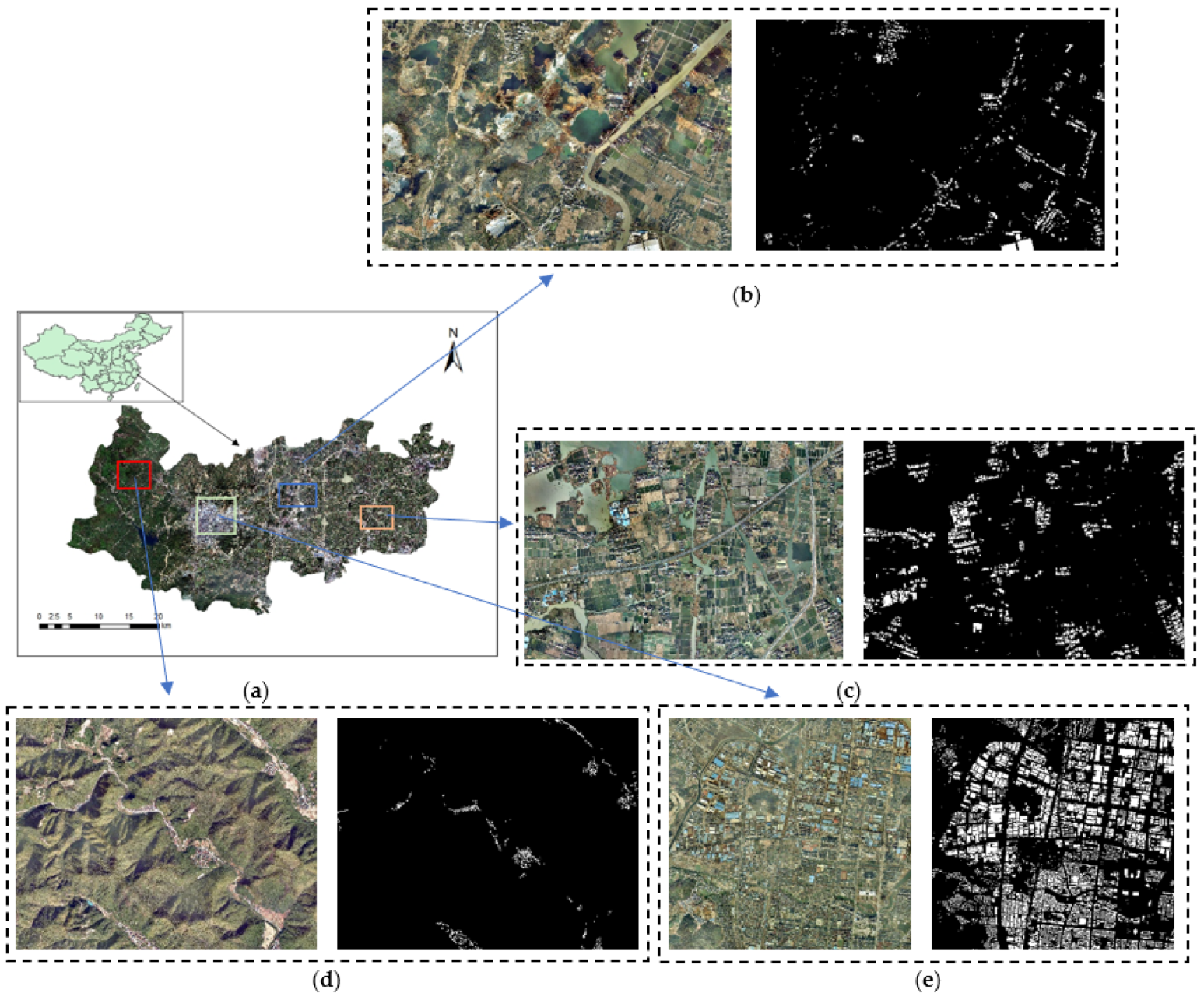
As one of the pilot counties for rural housing land reform, Deqing County, Zhejiang Province, China, has rich geomorphological characteristics. The west of Deqing County is a mountainous area, and the hilly area and plain area are located in the middle and the east, respectively. The features of homesteads in different geomorphic areas such as spatial distribution, texture, shape, and chromaticity are various. In order to apply the proposed approach in rural homesteads for future use, some representative geomorphological area images were selected as the study area (Figure 1).
2.2. Methodology
This study focuses on the extraction of rural homesteads in high-resolution remote sensing images and proposes a novel convolutional neural network, MBNet, for precise and automatic rural homestead statistics. Multiple branches in the network are designed for performing different tasks and then integrated for combining respective information. This section provides a detailed description of the network architecture.
2.2.1. Overview of Network Architecture
Given a high-resolution remote sensing image with three RGB channels, the encoder extracts the features and the decoder restores the resolution of the network, and finally, a binary image with the same length and width as the input image is output, where black areas denote background and white areas indicate homesteads.
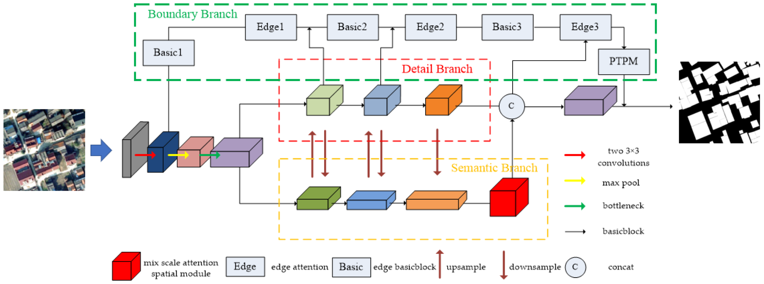
The proposed framework for refining the extraction of a homestead is shown in Figure 2. We use different colors to mark the feature map of different stages. The network encoder section mainly uses the BasicBlock module of ResNet-34 to extract features. However, the 7 × 7 down-sampling convolution module of ResNet is replaced with two 3 × 3 convolutions to reduce the number of parameters while maintaining the same receptive field, and these convolutions are then followed by the maxpool layer and the first bottleneck of ResNet-50. Extended from the basic modules for feature extraction, three branches are added to integrate more feature information: a detail branch (see Section 2.2.2), a semantic branch (see Section 2.2.3), and a boundary branch (see Section 2.2.4). The role of the detail branch is to maintain the low-level information such as edges and textures of small objects in the image. The semantic branch is used to extract high-level information in the image, allowing the algorithm to fully understand the image. The boundary branch is based on the detail branch to accurately extract the boundary of the object to refine the segmentation result.
2.2.2. Detail Branch
There is a contradiction in deep neural networks based on convolutional modules. The first few shallow neural networks have a higher resolution which can effectively maintain low-level information such as edges and textures, but the receptive field is narrow and lacks semantic information in the image. As the network gradually deepens, the deep network receptive field increases, and the semantic information becomes rich but with low image resolution, thus causing the detailed information loss of the image and the boundary blurring. This is challenging for some scenarios that require fine-grained semantic segmentation.
As illustrated in Figure 2, the detail branch is designed to keep the image resolution after down-sampling by four times. Through the fusion of the detail branch and semantic branch, the semantic information of the image can be fully understood while maintaining the detailed information of the image. In order to reduce the computational cost caused by maintaining the high resolution of the image, we use a simple BasicBlock as the feature extraction module, and the stride is 1. When acquiring the feature map sampled by the semantic branch, the high-resolution feature map and the low-resolution feature map are spliced, and then a 1 × 1 convolution layer is used to reduce the dimension, and the number of channels is set to 64. Batch normalization (BN) is used to normalize the data, and RELU is used as the activation function. The interaction between the detail branch and the semantic branch adopts a simple maxpool down-sampling and bilinear interpolation up-sampling method.
2.2.3. Semantic Branch
The semantic branch consists of a semantic feature extractor designed based on the last three layers of ResNet-34 BasicBlock and a mixed-scale spatial attention module in series. Since the ResNet is originally designed for classification tasks, the last two layers end with the global average pooling layer and fully connected layer, which is not applicable to dense pixel-based semantic segmentation tasks. Therefore, we remove the last global average pooling layer and fully connected layer. In the first BasicBlock and the second BasicBlock of the semantic branch, the feature map resolution is one-sixteenth of that of the original image after down-sampling the second BasicBlock with stride = 2. The last BasicBlock uses an atrous convolution with stride = 1 and atrous rate = 2 to increase the receptive field without reducing the resolution.
Mixed-Scale Module:
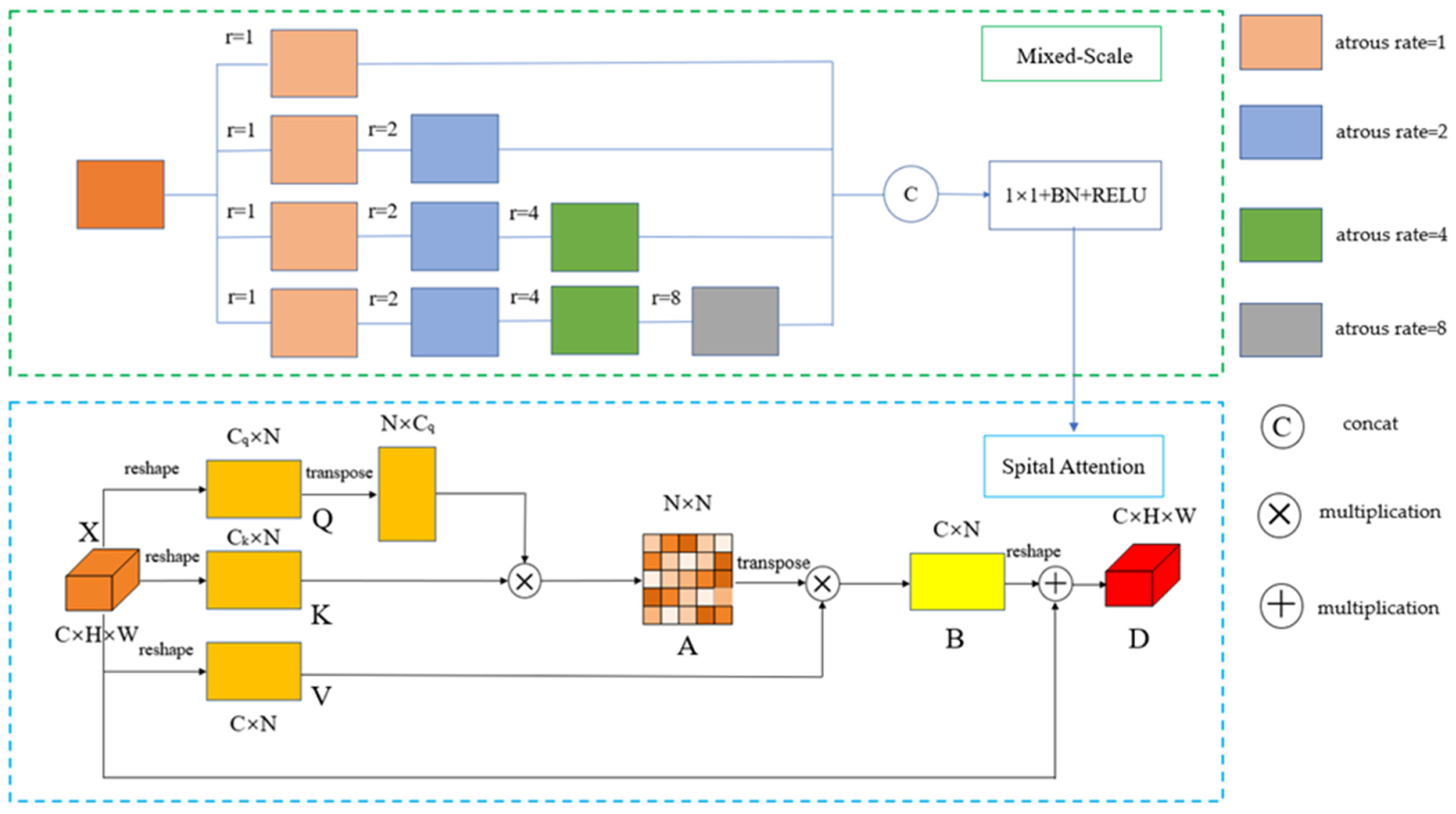
Inspired by atrous spatial pyramid pooling (ASPP) [27] and hybrid dilated convolution (HDC) [28], we designed a cascaded mixed-scale module. This module is composed of four groups of 3 × 3 convolution blocks with different atrous rates stacked. The fast atrous rate of the first group of convolution is 1, and the corresponding receptive field is 3; the atrous rates of the second group of convolution blocks are 1 and 2, and the corresponding receptive field is 7; the atrous rates of the third group convolution block are 1, 2, and 4, and the corresponding receptive field is 15; the atrous rates of fourth group convolution block are 1, 2, 4, and 8, and the corresponding receptive field is 31. The original input image size is 512 × 512, the feature encoder section of the semantic branch is down-sampled by 16 times, and the final output feature map size is 32 × 32. So, the feature points on the last center layer will present with 31 × 31 points on the first center feature map, covering the main parts of the first center feature map [29]. The obtained multi-scale feature maps are spliced with the 1 × 1 convolution for restoring the number of channels, and then the feature map after 1 × 1 convolution is input to the BN layer and RELU layer to normalize and activate mixed-scale features.
Spatial Attention Module:
The visual attention mechanism is a unique brain signal processing mechanism for human vision. Human vision obtains the target area that needs to be focused on by quickly scanning the global image and devoting more attention resources to this area [30]. The attention mechanism is inspired by the human visual system [30,31], which can establish long-range dependencies in space. It is widely used in computer vision tasks and natural language processing tasks [32,33,34,35,36]. The self-attention mechanism is an attention module originated in natural language processing [34], which associates the context information of different global positions and enhances the information representation by calculating the relationship between different positions in the sequence. The same idea is used in computer vision to aggregate image contextual information through a self-attention mechanism to highlight the importance of the foreground. The remote sensing images of rural homesteads are complex, and there are objects with a high similarity between classes, which are easy to misclassify. The self-attention mechanism can effectively help solve this problem. Combining the characteristics of the self-attention mechanism, we propose a spatial attention module.
As illustrated in Figure 3, given a feature map , we input it into a 1 × 1 convolutional layer to generate two new feature maps Q and K with channel numbers Cq and Ck, respectively, where , , and Cq and Ck are equal. Then the feature maps Q and K are reshaped to and , where . The transpose operation is performed on the feature map Q after the reshape operation, and the shape becomes . Next, we multiply K and the transposed Q matrix and generate the spatial attention feature map through the softmax function. A is defined as follows:
where is the scaling factor, which is used to prevent the back-propagation error of softmax from being 0 and the gradient disappearing when the variance is large. A is the size of the feature representation describing two spatial locations. The larger the value of A, the greater the correlation between them.
The feature map X generates a new feature map through the 1 × 1 convolution layer and also keeps the number of channels unchanged. Then it can be reshaped into shape and multiplied with the transposed matrix of the generated attention feature map A to obtain a feature map . Finally, we set a learnable scaling factor to adjust the weight of the attention feature map B and reshape it into , which is added to the input feature map X pixel by pixel to form the final feature map :
where is initialized as 0, and the optimal value is obtained by continuous learning [37].
For semantic segmentation, contextual information is very important for understanding semantic information [38]. The spatial attention mechanism weights each position of the multi-scale feature map output by the mixed-scale module to generate a multi-scale attention feature map, which makes the model pay more attention to foreground objects, suppresses the interference of non-foreground objects with the foreground, and enhances the representation ability of the foreground pixels, so as to achieve the understanding of the scene environment and semantics in the remote sensing image.
2.2.4. Boundary Branch
The allocation of pixels in semantic segmentation tasks is unbalanced. Generally, only a small number of pixels are located at the boundary of the object, and the number of pixels in the main part of the object is much larger than the number of pixels on the boundary, which leads to the lack of attention of the semantic segmentation model to the boundary. It is difficult for the end-to-end semantic segmentation model to accurately identify the edge contours of objects. It is far from satisfactory to segment objects only by predicting the body part. Therefore, we propose an edge branch that is learned individually based on fusion modules.
Figure 2 shows the overall process of the boundary branch, where the high-resolution (4×) feature maps and low-resolution semantic feature maps are concatenated to form a feature fusion module, on which low-level texture information and high-level semantic information are learned to generate the boundary feature map. Here, we retain the edge detail information of the stem module and use the high-resolution semantic feature maps of the first, second, and third modules of the detail branch to generate the boundary attention module, which then can be used to weight the boundary feature maps from the stem. The steps are as follows:
- (1)
- Obtain the feature map output by the stem module as the main feature, up-sample to the original image size, and go through a 1 × 1 convolutional layer. Then input it into BasicBlock and use 1 × 1 convolution to reduce the dimension to half the number of original channels;
- (2)
- Reduce the fused feature map from the first module of the detail branch to a single channel, and then up-sample the result to the original image size;
- (3)
- Concatenate the feature maps obtained in the first step and the second step, reducing the dimension to a single channel after the BN layer and RELU activation, and use the sigmoid function to generate the boundary attention mechanism (BAM):
- (4)
- Reduce the edge feature map after the current weighted semantic information from the residual function according to ResNet’s residual paradigm:
- (5)
- Take the feature map generated in step 4 as the main feature, and cycle the above steps to the feature map which is concatenated by the last step in the detail branch and semantic branch.
- (6)
- The final boundary generated in step 5 is input to the feature which is concatenated by the last layer of the detail branch and the semantic branch. Then input the final boundary map to point-to-point refinement module (PTPM) for correction processing to obtain the final accurate semantic boundary. The specific point-to-point module will be described next.
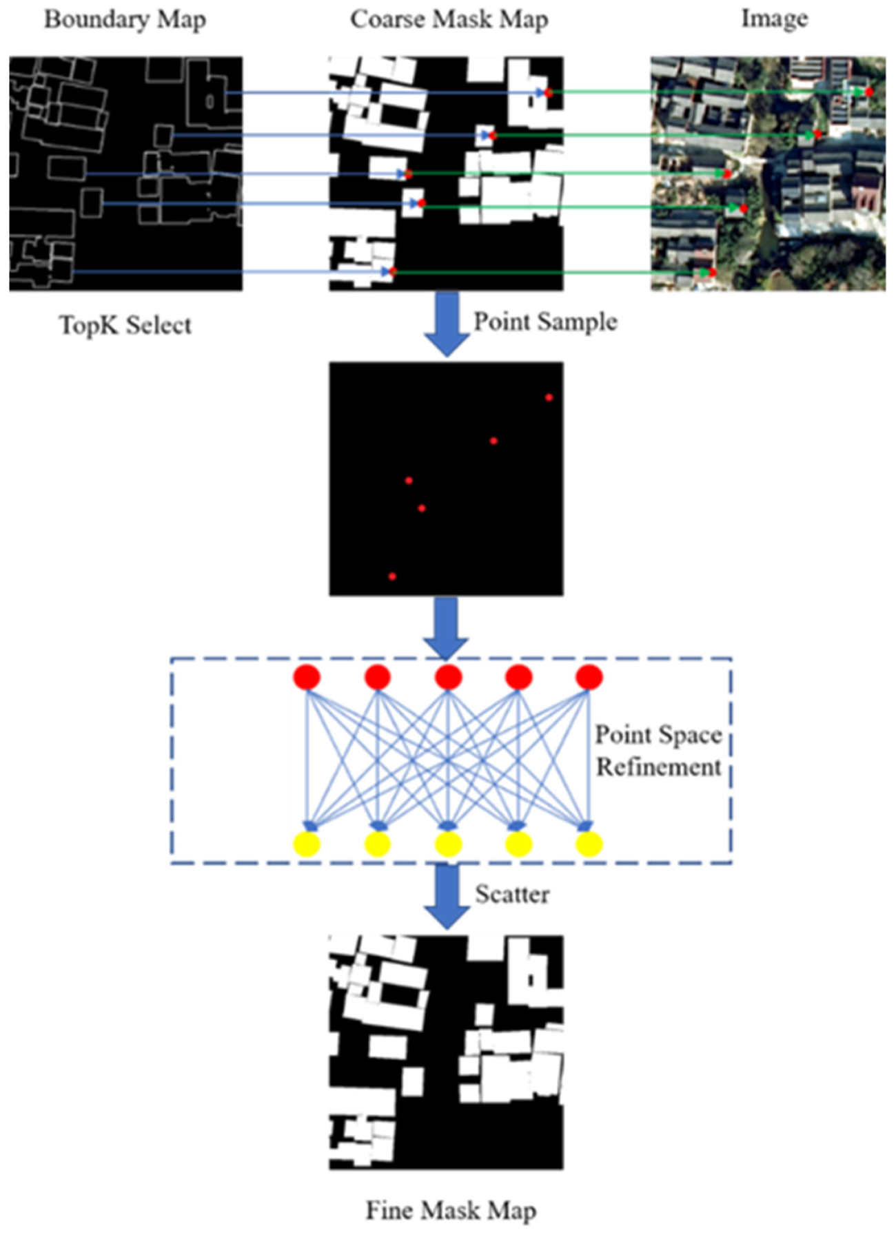
Point-To-Point Module:
In order to achieve finer boundary delineation on the final semantic segmentation result map, we designed an efficient point-to-point module (PTPM) to refine the boundary. The key of PTPM is to extract the predicted accurate points and uncertain points from the precise boundary, establish the spatial relationship between these points and the semantic segmentation map, and obtain the boundary point affinity map of the semantic segmentation map.
As illustrated in Figure 4, we first select the K points with the highest confidence and another K points with the lowest confidence from the predicted semantic boundaries (the value of K in this paper is 2048), and then we calculate the position coordinates of these 2K points and map them to the coarse mask map. The corresponding points are indexed by position coordinates and samples to establish the point-to-point spatial relationship. The matrix shape of these points is 2K × C, where C is the number of channels. Then we input the matrix of shape 2K × C into the point space refinement module for re-prediction, update the parameters of the MLP through back-propagation of the loss function, and iteratively obtain the correct category of the boundary points in the mask map. Finally, the correct boundary points are remapped to the coarse mask map to obtain the fine mask map. It should be noted that the optimization network in PTPM is a fully connected network composed of 1 × 1 convolutions, which can also be understood as an MLP structure.
2.2.5. Loss Layer Design
The proposed network architecture is a kind of multi-task learning, which can be roughly divided into detail semantic tasks and boundary tasks. Therefore, the loss function consists of two parts: semantic loss and boundary loss. Although some semantic segmentation networks based on the encoder–decoder structure have adopted deep supervision methods and achieved good results [19,39,40,41,42,43], adopting multi-layer supervision will significantly increase the amount of computation, and in this experiment, it is also found that the recognition results are not significantly improved by adopting the deep supervision method. Therefore, the loss calculations are designed on the last layer of feature maps.
Semantic Loss:
Binary cross-entropy loss (BCE) is the most widely used loss function in binary classification tasks [44]. It is defined as:
where and represent the ground truth and the predicted probability map of a pixel. N is the total number of pixels.
Data imbalance is a common problem in data analysis, deep learning, and other fields. Although the BCE loss is relatively stable, when the data are unbalanced, it will cause the loss function to drop rapidly in the direction of a large number of categories, resulting in ignoring other categories. For remote sensing image semantic segmentation tasks, data imbalance is almost unavoidable, especially for tasks such as building extraction in rural areas. Despite the data resampling operation being performed, the number of foregrounds is still smaller than the number of backgrounds in most cropped images. So, we need to use weighted BCE loss to rebalance the data. We use the hyperparameter to define the weighted BCE loss:
where is a parameter that weights positive samples and is a parameter that weights negative samples. In this work, is set to 0.85 and the value of is 0.15.
Boundary Loss:
The loss function of the boundary branch consists of two parts. One part is the weighted BCE loss function, and the other part is the Dice loss to obtain a clear boundary.
There is a serious imbalance between boundary pixels and non-boundary pixels. In order to avoid training collapse caused by data imbalance, we use the weighted BCE loss of Formula (6) and set the weight of the boundary loss as
where represents the boundary pixel; , , and represent the number of non-boundary pixels, the number of boundary pixels, and the total number of pixels, respectively.
Due to the serious imbalance of the number of pixels on the boundary and the non-boundary, as well as the nearest neighbor interpolation in the upper process, the final predicted boundary is very thick and not clear enough. The ideal boundary is composed of a single pixel, and too thick a boundary will cause inaccurate segmentation results. Inspired by LPCB [45], we add Dice loss [46] to the boundary loss function to ensure that the shape of the boundary is consistent with the ground truth, making the predicted boundary thinner. The basic expression of Dice loss is shown in Equation (8):
where N denotes the total number of pixels in the image and yi denotes whether the ith pixel in the ground truth belongs to a homestead. If it belongs to a homestead, yi = 1; otherwise, yi = 0. pi denotes the probability that the ith pixel in the predicted result is a homestead.
Joint Loss:
To constrain the consistency of multi-branch learning, we assign weights to each loss function and add them to obtain the final joint loss function, which is defined as follows:
where is the weight of the semantic segmentation loss and and are the weights of the boundary loss. In this study, we set , , and to 1, 25, and 1, respectively.
3. Results
In this section, we describe the method of processing the dataset in experiments and then provide experimental parameter settings and quantitative evaluation methods. Finally, we compare the quantitative evaluation results of the proposed method with those of other state-of-the-art methods and analyze the reasons leading to these results.
3.1. Dataset
The dataset in this study covers the entire county areas of Deqing County, and the remote sensing images have rich landform features, including mountainous landforms, hilly landforms, and plain landforms. The distribution and characteristics of homesteads in different landforms vary greatly. Different kinds of datasets are divided for analysis and comparison according to the characteristics of the landforms. In addition, a suburban homestead is different from the above; it is larger and relatively regular, and also closely arranged, so it is also added as a separate dataset.
The original remote sensing image is labeled with LabelMe to generate a mask. In order to train the boundary branch, we generate ground truth through the distance map transform method [47]. Specifically, we calculate the Euclidean distance between each pixel in the image and the background point (pixel value is 0) to obtain a binarized segmentation mask map and then set a threshold, and points smaller than the threshold are considered as boundary points. Here, we set the threshold to be .
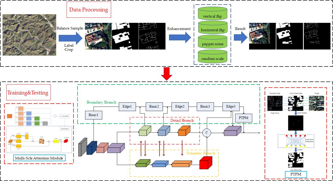
Since the GPU memory cannot accommodate large-sized remote sensing images and labels, we crop the image to 512 × 512 pixels. Considering that there are data imbalance and multi-scale problems in the dataset, and in order to expand the dataset, the cropping strategy is divided into two steps:
- Starting from the upper left corner of the image, the number of clipping sliding steps is 256. When cropping to a certain area, the number of background pixels/total number of pixels ≤ 0.92, and then the number of sliding steps is reduced by half; otherwise, the number of sliding steps is multiplied by 0.9 and then rounded up.
- After randomly cropping the image; if the number of background pixels/total number of pixels ≤ 0.9, it is kept; otherwise, it is discarded.
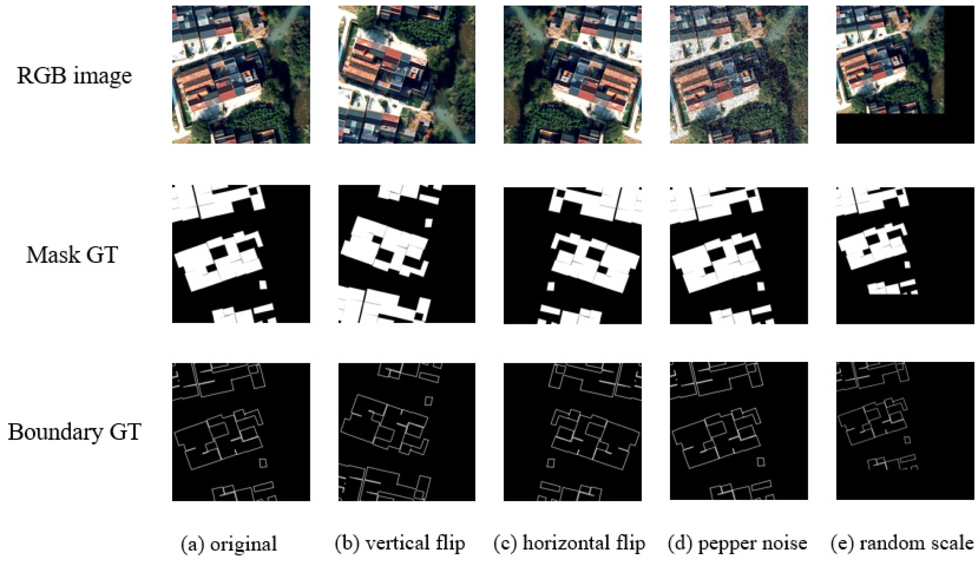
As shown in Figure 5, we perform data modification according to a certain probability during training for each cropped image, including random scaling, random horizontal and vertical flipping, random salt and pepper noise, random color dithering, etc.
3.2. Experimental Setting
All of the experiments in this paper were implemented based on the PyTorch framework. The network was initialized with He_normal [48] instead of using pretrained weights. We chose the SGD algorithm with momentum as the optimizer and set the momentum to 0.9 and the initial learning rate to 1 × 10². The learning rate decay follows the following rules:
where base_lr is the learning rate of the last update, cur_iters is the current number of steps, max_iters is the total number of training steps, and the value of power is set to 0.9.
All experiments were processed on a Linux server with 128 GB RAM and 6 × 16 GB Tesla P100 GPUs. The batch size was 4 on each GPU, and the batch size for each training was 16.
3.3. Evaluation Metric
In order to accurately evaluate the performance of the proposed method in this paper, we selected five evaluation metrics commonly used in the field of semantic segmentation, namely OA, precision, recall, F1-score, and IOU. F1-score is also used to evaluate the effect of the boundary. Their definitions are as follows:
where TP (true positive) denotes the correctly identified homestead pixels, FP (false positive) denotes false predictions on positive samples, FN (false negative) denotes false predictions on negative samples, and TN (true negative) denotes the correctly identified background pixels.
3.4. Comparisons and Analysis
To verify the performance of MBNet, we contrasted the performance and also completed ablation experiments on the dataset. First, we compared the performance of MBNet with several state-of-the-art (SOTA) algorithms. Then, we performed boundary branch ablation experiments to compare the performance of the network with and without the boundary branch. In addition, we conducted refined loss ablation experiments to compare the performance of the network under different losses.
In this study, we compared MBNet with six SOTA algorithms, namely FCN-ResNet [6], UNet-ResNet [7], DeepLabV3+ [8], HRNetV2 [49], MAP-Net [50], and DMBC-Net [51]. The first four are general SOTA models in the field of computer vision, and the latter two are the latest building semantic segmentation models for remote sensing images. Considering the fairness of the comparison, the backbones of the models we choose to compare are almost all based on the ResNet paradigm. As the pioneering work of semantic segmentation, FCN has been widely applied in many aspects. U-Net is a typical encoding–decoding structure model that integrates the underlying information and is more friendly to boundary processing. DeepLabV3+ is the latest version of the DeepLab series, using ResNet-50 as the backbone, in which the ASPP structure can fully learn multi-scale information. HRNetV2 is a recent SOTA model in the field of convolutional neural networks; it learns multi-scale semantic information while maintaining resolution. MAP-Net learns spatially localized preserved multi-scale features through multiple parallel paths and uses an attention module to optimize multi-scale fusion. DMBC-Net learns semantic information and boundary information through multi-task learning and uses boundary information to optimize the segmentation effect.
For a fair comparison, we adopted the same initial learning rate, number of training steps, optimizer, and other hyperparameter setting strategies during training. In addition, we also analyze the results at the end of this section.
3.4.1. Comparison with SOTA Methods on Mountain Landforms
As shown in Table 1, the proposed method achieves the best results of all methods. All quantitative evaluation indicators of MBNet surpass those of other methods, and also the visual effect of segmentation is the best. Compared with HRNetV2, which is the best general algorithm in the computer vision field, MBNet is 1.66%, 1.61%, and 1.37% higher in IOU, recall, and F1-score, respectively. Compared with DMBC-Net, which is specially designed for building extraction, MBNet is 0.89%, 1.15%, and 0.60% higher in IOU, recall, and F1-score, respectively.
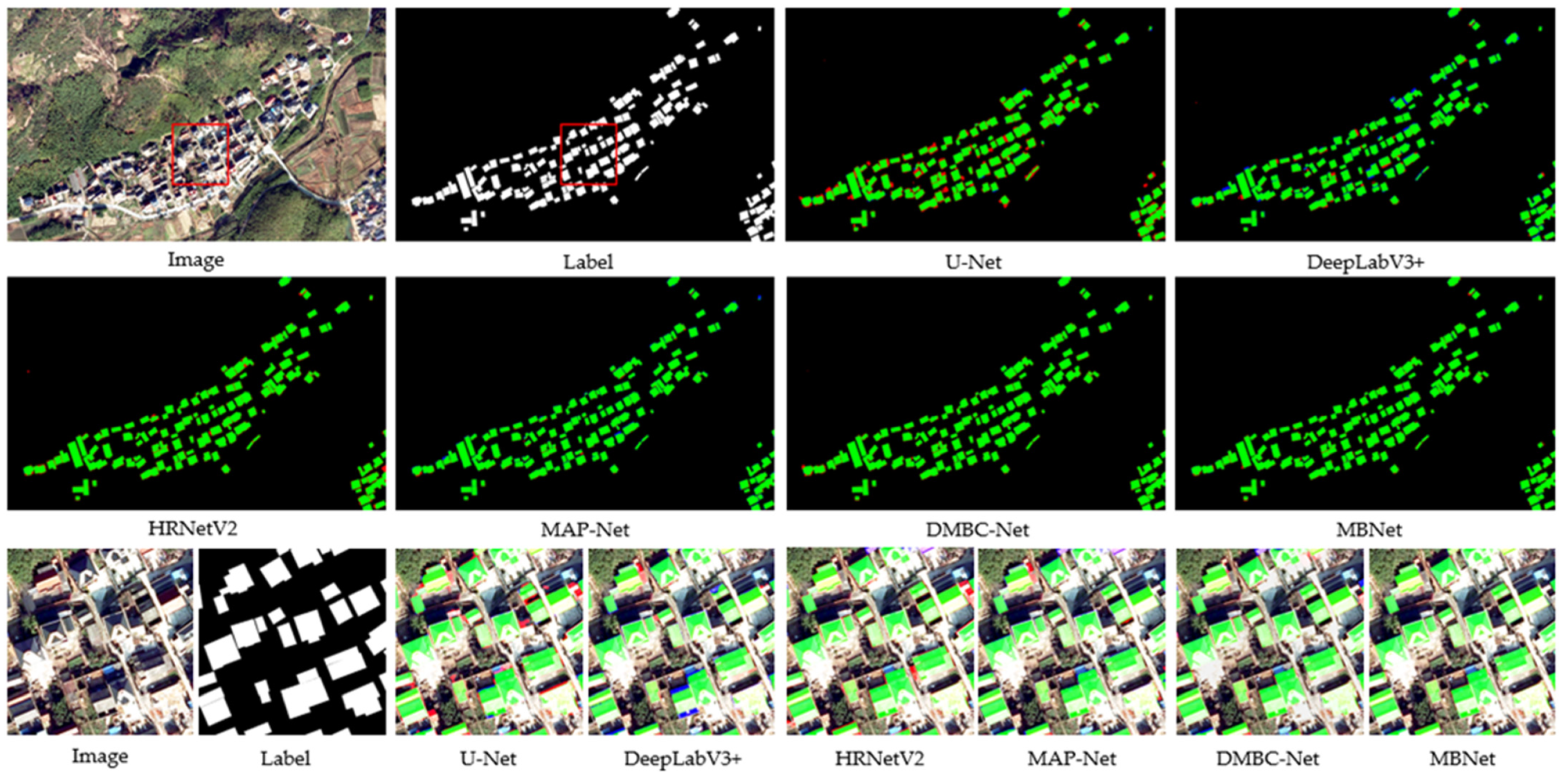
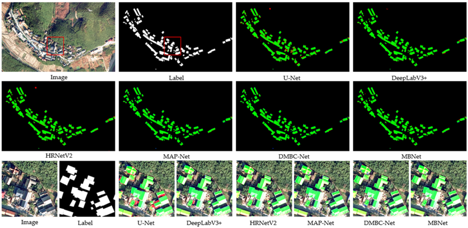
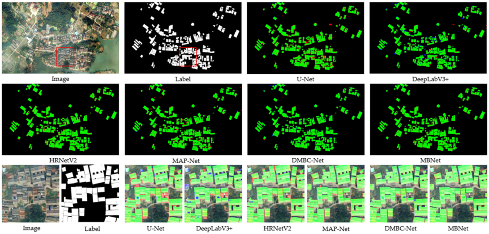
Figure 6, Figure 7 and Figure 8 show some example results of extracting rural homesteads on mountainous landforms by different methods. The extraction of homesteads on mountainous landforms is simpler than on other landforms, and thus HRNetV2, MAP-Net, and DMBC-Net perform well in the extraction effects, but there are some defects in the boundary. Although HRNetV2 always maintains high resolution, it lacks fine processing of boundaries, so some complex boundaries cannot be correctly identified. Despite average pooling and larger atrous rate used in MAP-Net and DMBC-Net to extract contextual information, the detailed homestead information is easily ignored, which destroys the continuity of their texture structure and geometric information. This is more evident in DeepLabv3+, resulting in more FNs in DeepLabv3+. In contrast, the MBNet extraction results have more correct and complete boundaries. The interaction between the detail branch and the semantic branch of MBNet makes the underlying image with high resolution contain rich semantic information. At the same time, the boundary branch extracts fine boundaries from the detail branch rich in semantic information to improve the boundary effect of the segmentation results. Since FCN and U-Net lack the ability to aggregate multi-scale semantic information from context and have a weak semantic understanding of images, some shadows and roads similar to the color and texture of homesteads are misidentified as homesteads, which leads to more FPs.
3.4.2. Comparison with SOTA Methods on Plain Landforms
Table 2 shows the quantitative evaluation results of rural homestead extraction on plain landforms. Due to the complexity of the plain landform scene, the variety of ground objects, and the diversity of homestead texture structures, homestead extraction on plain landforms is more difficult than on other landform types; nevertheless, MBNet is still the best in terms of visual effects and in quantitative evaluations. Compared with HRNetV2 and DMBC-Net, MBNet achieves higher IOU and F1-score, respectively.
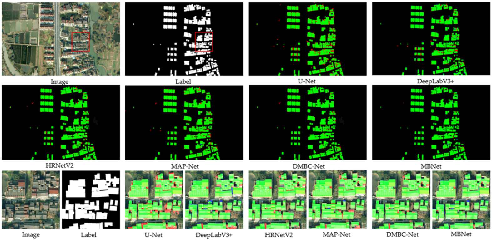
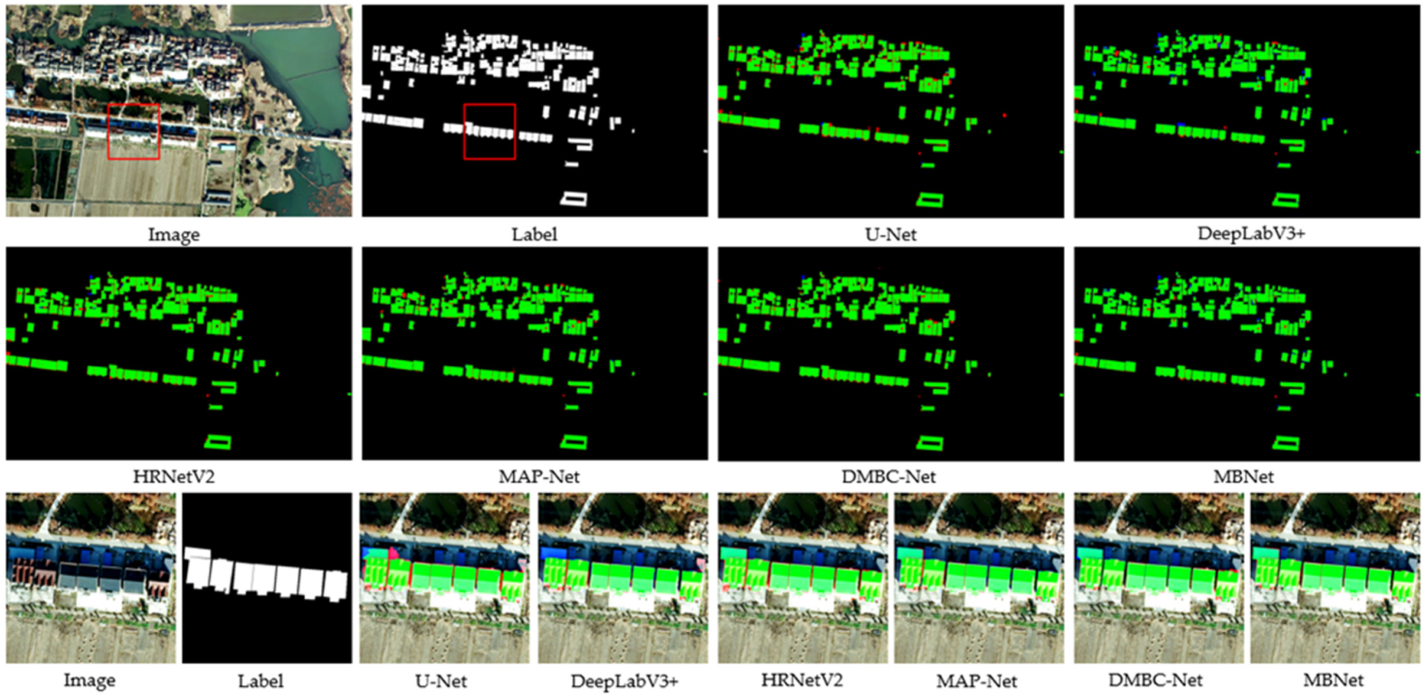
Figure 9, Figure 10 and Figure 11 show some example results of extracting rural homesteads on plain landforms by different methods. Plain landforms contain a large number of non-homestead objects whose spectrum is similar to homestead, including shadows of buildings, farmland, and roads. These background objects can be easily identified as homestead objects. In addition, the buildings have a complex texture structure and are closely arranged, and two adjacent homesteads can easily be identified as the same object. Because FCN and U-Net networks do not have the ability to aggregate contextual multi-scale information, these misleading background objects are easily marked as homesteads, so a large number of FPs are presented in the results. DeepLabv3+ ignores many details of homesteads due to the large atrous rate. Similarly, DMBC-Net also suffers from this problem, but the existing boundary constraints improve the effect of homestead extraction. The ability of HRNet to extract multi-scale information and fusion is insufficient, and some contexts are easily identified as homesteads. Furthermore, due to the existence of multi-scale average pooling in MAP-Net, the details and small objects at the boundary are blurred. By comparison, the proposed MBNet addresses these issues using multiple branches. The mixed-scale spatial attention module of the semantic branch aggregates the multi-scale information of the context and weights the background and objects to highlight the more important foreground objects. The detail branch and the boundary branch are used to extract the refined semantic boundary of the homestead, which helps improve the segmentation results.
3.4.3. Comparison with SOTA Methods on Hilly Landforms
Table 3 shows the quantitative evaluation results of rural homestead extraction on hilly landforms. The hilly landform scene is similar to the plain area, and there are many types of homestead texture structures. However, the remote sensing images are not as clear as those of plain landforms due to clouds and fog. This creates a new challenge for extracting homesteads. For the quantitative evaluation of various methods, MAP-Net and MBNet are the least affected by cloud disturbance, and MBNet has the best quantitative evaluation result. Compared with HRNetV2, MBNet is 1.37% and 1.02% higher in IOU and F1-score, respectively. Furthermore, compared with MAP-Net, MBNet is 0.72% and 0.24% higher in IOU and F1-score, respectively.
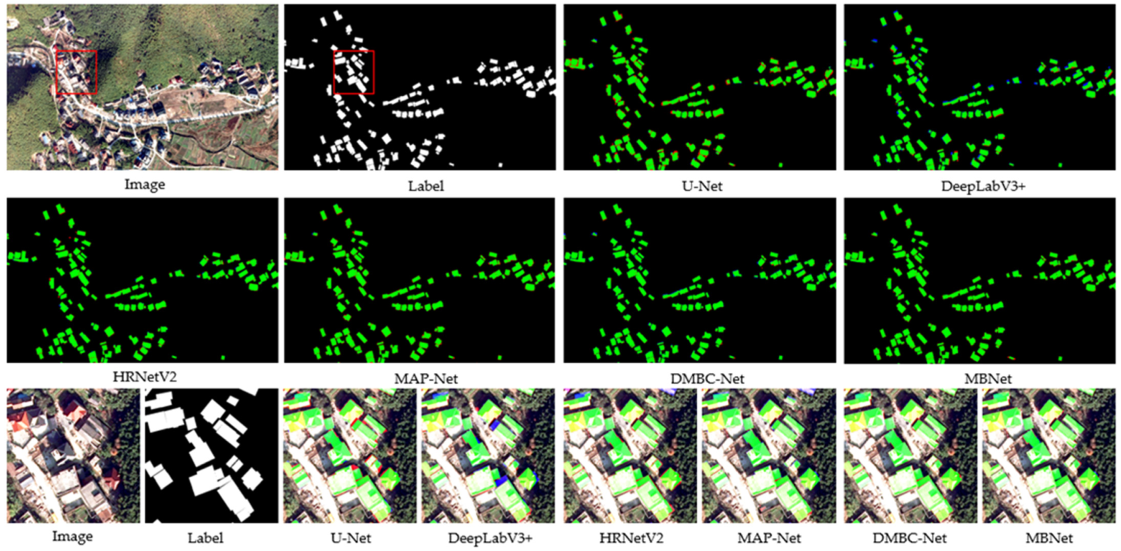
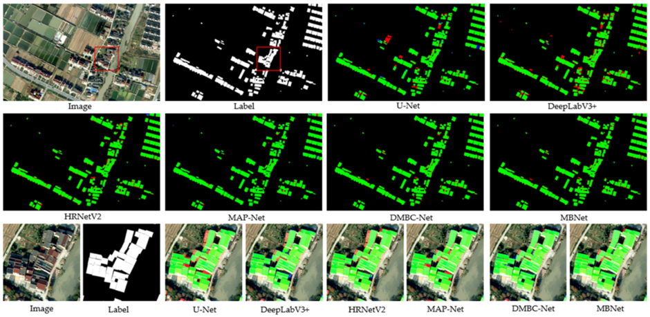
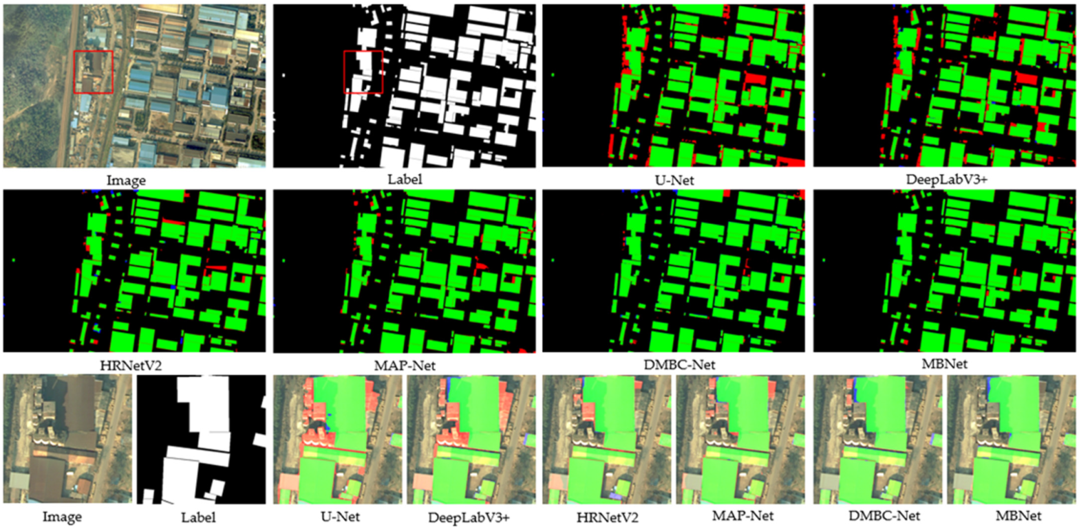
Figure 12, Figure 13 and Figure 14 show some example results of extracting rural homesteads on hilly landforms by different methods. Although the hilly landform is similar to the plain landform scene, the overall evaluation result is inferior to that of the plain landform due to the presence of clouds and fog in the images of some hilly landforms. This helps evaluate the robustness of the proposed algorithm in different complex scenarios. As can be seen from Figure 12 and Table 3, the segmentation results of FCN and U-Net are greatly affected by the clouds and fog, and the value of IoU drops significantly. This can be attributed to the lack of multi-scale aggregation modules, and the semantic information of images cannot be fully understood. However, the MAP-Net is not affected, and instead the IoU value increases. This is because the channel attention squeeze module works in the network. Specifically, this module can weight the foreground objects in the channel dimension and is insensitive to changes in the color channels of the image. Therefore, the mixed-scale spatial attention module in the proposed MBNet is weighted from the spatial dimension. When the pixel information under the clouds and fog cannot be understood, the semantic information can be understood through other surrounding and long-range pixels, which reduces the influence of clouds and fog on the image. The influence of clouds and fog shows that the proposed model has strong robustness. The precise boundary results predicted by the detail branch and the boundary branch improve the segmentation effect, making the prediction results of MBNet the best.
3.4.4. Comparison with SOTA Methods on Suburban Landforms
Table 4 shows the quantitative evaluation results of rural homestead extraction on suburban landforms. Compared with the above three landforms, homesteads in the suburbs are distinct, and they are more like buildings in urban areas which are regular in shape, densely arranged, and numerous. However, there are many types of homesteads, and there are a large number of background objects with a similar spectrum. All quantitative evaluation metrics of the proposed MBNet are the highest in the test set, which is consistent with the conclusion reached for the other three landforms. Compared with HRNetV2, MBNet is 2.37%, 1.06%, and 1.29% higher in IOU, recall, and F1-score, respectively. Compared with DMBC-Net, MBNet is 0.89%, 0.46%, and 0.61% higher in IOU, recall, and F1-score, respectively.
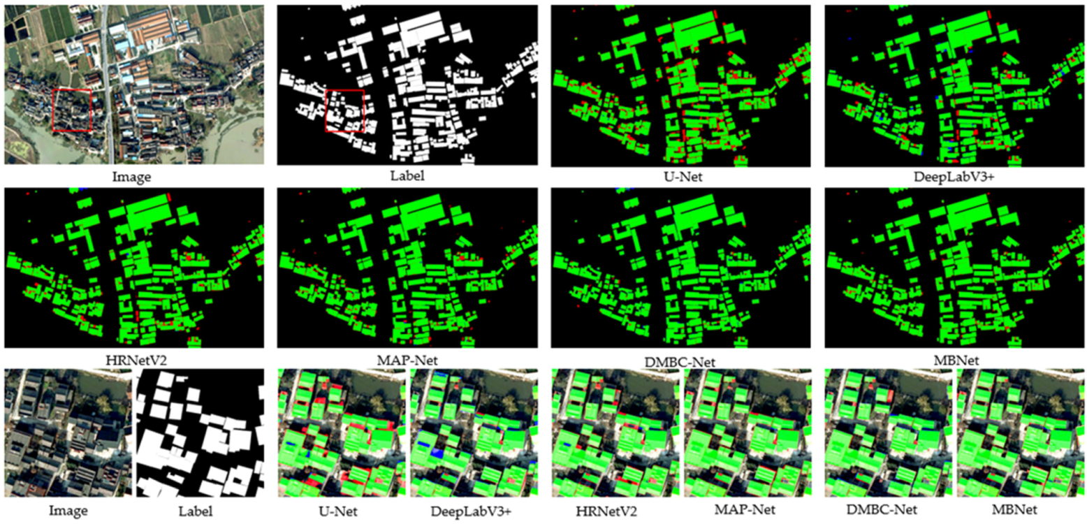
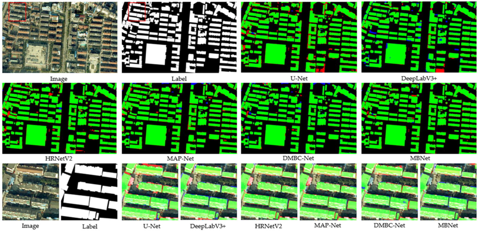
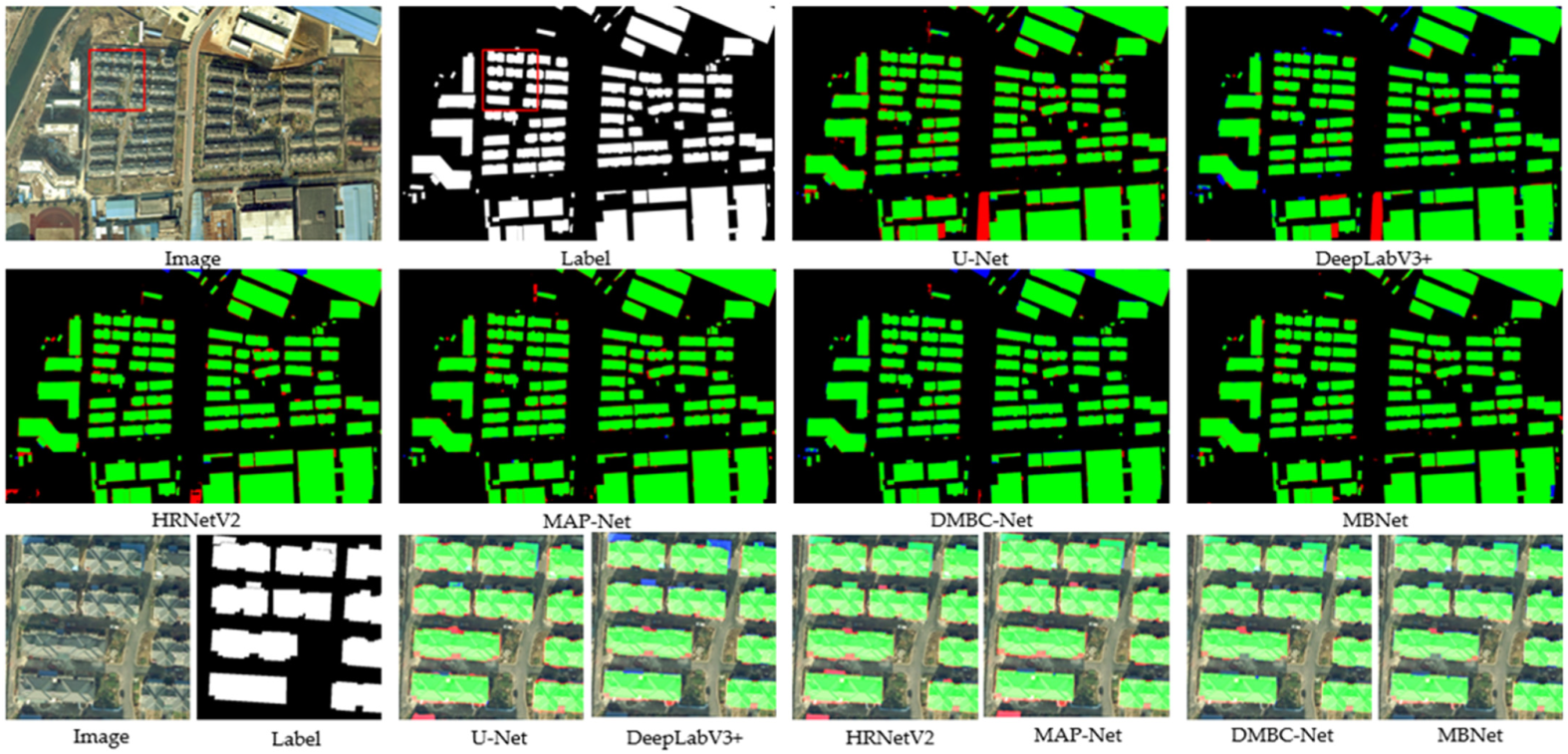
Figure 15, Figure 16 and Figure 17 show some example results of extracting rural homesteads on suburban images by different methods. The homesteads have a large proportion in the suburb image, which helps provide more targets for the training model. However, there are many types of homesteads in the suburbs, and there are a large number of non-homestead background objects with a similar spectrum and texture to homesteads, such as the ceiling in Figure 15, which can be easily identified as homesteads. Moreover, the houses have various contours and irregular shapes, and the predicted result boundary is not accurate enough. For FCN and U-Net methods, the lack of contextual multi-scale modules makes them weak in understanding image semantic information, and they are likely to identify shadows and ceilings as homesteads. The atrous rate design of DeepLabV3+ makes it easily ignore many details, resulting in the omission of many homestead objects. However, the multi-scale aggregation ability of HRNet is not sufficient, and it lacks a deep understanding of semantic information, which produces many misidentifications. Due to the mixed-scale spatial attention module of MBNet, the receptive field of MBNet covers the whole image, and it pays more attention to the foreground area. Therefore, the understanding of context semantics is better than that of MAP-Net and DMBC-Net, and there are fewer misidentifications. Compared with other models, the boundary improvement module of MBNet has an obvious effect on the extraction of homesteads in the suburbs. Figure 15 and Figure 16 demonstrate the boundary extraction ability of MBNet, and it can be seen that the boundary of MBNet is the most complete with the highest accuracy.
4. Discussion
In this section, we will discuss the effect of the mixed-scale spatial attention module and the refine module of the boundary branch on the performance of the network. For the mixed-scale spatial attention module, we use a heatmap visualization method to verify its effectiveness. For the refine module of the boundary branch, we use ablation experiments to verify its improvement on the network. The experimental data and experimental parameter settings are consistent with Section 3.1 and Section 3.2.
4.1. Visualization Experiment of Mixed-Scale Spatial Attention Module
The scenes in remote sensing images are complex, and there are similar phenomena in spectrum and texture between different objects. For the task of automatic extraction of refined homesteads in remote sensing images, the algorithm needs to deeply understand the information represented by pixels on the image and eliminate background interference objects such as shadows, ceilings, and clouds. Understanding the semantic information of an image needs to be learned from the global receptive field. Traditional networks such as AlexNet, VGGNet, and ResNet increase the receptive field by continuous down-sampling until the global receptive field is reached, but this will reduce the resolution and cause the details of the image to be blurred. In order to solve this problem, we adopt the method of multi-layer hole convolution in series and then in parallel as shown in Figure 3, which covers the global receptive field of the image while maintaining the image resolution and learning information from multiple scales. The spatial attention module can capture the spatial dependency between any pixel point in the image and other pixel points, and it uses the correlation between points to weight the spatial modeling of the foreground target, which can obtain more discriminative features and enhance the explicit representation of foreground objects in an image. This is the reason why the proposed method achieved excellent performance for homestead extraction on hilly landforms. To better illustrate the importance of the mixed-scale spatial attention module, we visualize the learned multi-scale attention map.
The proposed model highlights the homestead in Figure 18, and the results indicate that if the homestead has a larger proportion of the image, the model pays more attention to the homestead. In the attention map, the model also pays more attention to indistinguishable homesteads, which are often in shadow, obscured by vegetation, or at the edge of the image. The red boxes in the first and second rows show the model’s attention to the homestead covered by shadows. The red box in the third row shows the model’s attention to the homestead covered by vegetation, and the red box in the fourth row shows the model’s attention to the homestead located at the edge of the image. The visualization results show that the mixed-scale spatial attention module is able to capture long-range spatial dependencies of image semantics.
4.2. Boundary Branch Ablation Experiment
We use MBNet as the backbone to verify the effectiveness of the boundary branch by comparing the results of adding and deleting it. Convolutional neural networks need to continuously increase the receptive field when extracting high-level semantic features, and this process is often accompanied by a reduction in resolution, which is unfriendly to tasks that require precise edge information. By paralleling the detail branch and the semantic branch, MBNet retains the low-level information such as the boundary and texture of the image when fully understanding the semantic information of the image. However, due to the lack of active guidance and constraints on the boundary information, the boundary information is still imprecise. To obtain accurate boundary information, we design a boundary branch to refine the segmentation results by directly guiding the learning of boundaries.
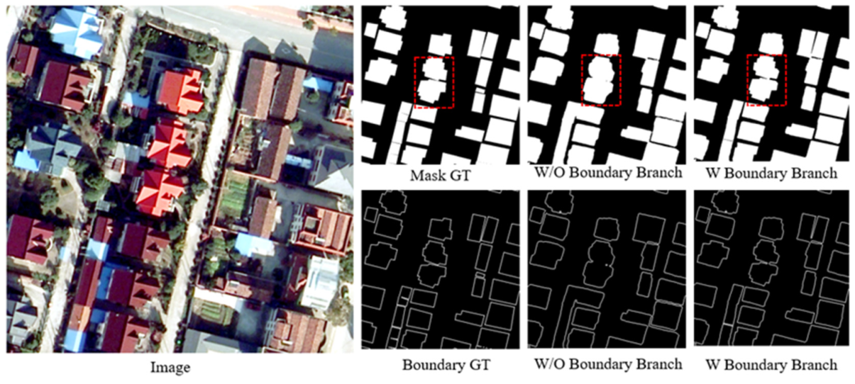
Table 5 and Figure 19 show the results of MBNet with and without the boundary branch. It should be noted that, in order to verify the role of the boundary branch of MBNet, we do not conduct experiments with different landforms alone. The results in Table 5 are the average of the results for various landforms. It can be seen that both the segmentation effect and the quantitative evaluation indicators of MBNet with the boundary branch added perform better than those of MBNet with only the detail branch and semantic branch. In the mask segmentation results of Figure 19, the red boxed part of MBNet with the boundary branch is more in line with the contour of the homestead than MBNet without the boundary branch. Further, two separate homesteads can be identified instead of recognized as one case, which can also be seen from their boundary prediction plots. Accurate boundaries are of great significance for the statistics of quantitative indicators such as the numbers and areas of homesteads. This illustrates the ability of the boundary branch to improve the semantic segmentation results of other branches.
4.3. Point-to-Point Module (PTPM) Ablation Experiment
In order to verify the effectiveness of PTPM, we added and removed it in the boundary branch and also chose different point-taking strategies. There are three different point selection strategies: select the K points with the highest confidence, select the K points with the lowest confidence, and select a total of 2K points both with the highest and the lowest confidence at the same time. Through the experiments, we found that although Dice loss can make the predicted edges clearer, it cannot achieve single-pixel accuracy. When two homesteads are close to each other, two adjacent sides are often glued together because the edges are not thin enough, which will cause an inaccurate segmentation result in semantic segmentation and prevent distinguishing between adjacent homesteads. We observed that the K points with the highest confidence are located at the correct boundary positions of the image, and the K points with the lowest confidence are often located in the areas where the edges are not thin enough to cause adhesion, so these points are selected in the semantic segmentation map for retraining. The results are shown in Table 6 and Figure 20.
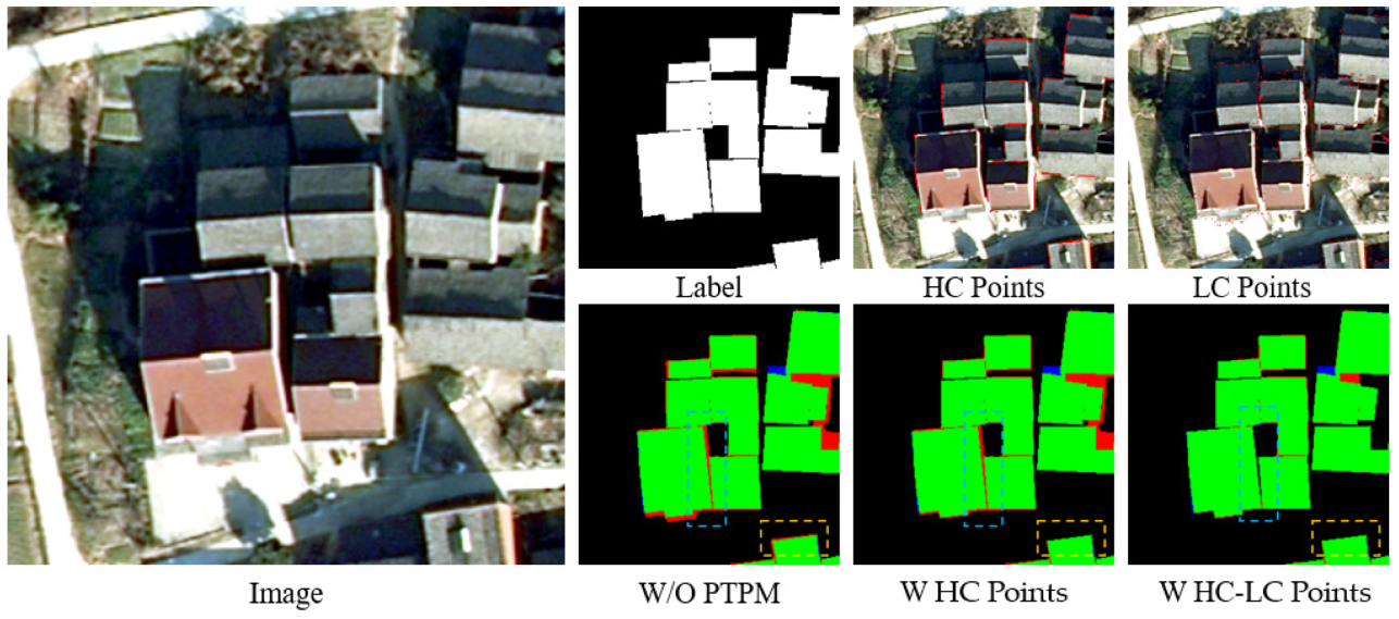
Table 6 and Figure 20 show the results of MBNet with and without the PTPM. It can be seen from the figure that the points with high confidence are relatively dense and concentrated and are located at the edge of the homestead, while the points with low confidence are scattered and distributed in the shadows and closely connected places that are difficult to identify. The yellow box represents the prediction result plus the points with high confidence. It can be seen that the boundary is finer and there are fewer FPs. The blue box indicates that the prediction results of points with low confidence are added, and two closely adjacent homesteads can be distinguished, which is of great significance to the accurate statistics of the number of homesteads. The results in this section illustrate the improvement of the network by the PTPM.
5. Conclusions
In this paper, we propose a multi-task learning framework, MBNet, with a detail branch, a semantic branch, and a boundary branch for rural homestead extraction from high-resolution remote sensing images. Usually, semantic segmentation tasks need to learn high-level semantic features through continuous down-sampling, but this will reduce image resolution and destroy image details. In order to keep the detail information, this paper designs a detail branch, which maintains the resolution of the image after down-sampling by 4 times. At the same time, for obtaining multi-scale spatial aggregation information, this paper designs a semantic branch and adds a mixed-scale spatial attention module at the end of the semantic branch to extract multi-scale information and enhance information representation. In addition, this paper also designs a boundary branch to maintain the consistency of the boundary and ground truth. This branch obtains boundary information and optimizes the boundary information of the segmentation map through the point-to-point module (PTPM). We conducted experiments on UAV images in Deqing County, Zhejiang Province, to verify the effectiveness of the proposed method. Deqing County is divided into mountainous landforms, plain landforms, and hilly landforms. Considering the differences in homesteads, we added the suburbs in the densely populated areas as one of the experimental objects, and the complex terrain environment as well as the dense rural buildings can help verify the applicability and robustness of the proposed method. The experimental results show that our method achieves better results than other advanced methods and can extract the homesteads accurately from the remote sensing images, which lays a foundation for the quantitative research of homesteads. Our research has verified the effectiveness of MBNet in experiments. MBNet can be applied to end-to-end extraction of dense rural homesteads on satellite or UAV images. Furthermore, MBNet can also be used to extract dense and difficult-to-recognize features in the image. In future work, we will consider the instance objects of rural homesteads from the perspectives of self-supervision and weak supervision, and we will describe each instance object with the method of instance segmentation.
Author Contributions
R.W. and Z.Z. conceived and conducted the experiments and performed the data analysis. A.Z. assisted in collating experiment data. R.W. wrote the article. Y.W. and B.F. revised the manuscript. All authors have read and agreed to the published version of the manuscript.
Funding
This research was supported by the Innovation Research Fund of Agricultural Information Institute of CAAS, China (CAAS-ASTIP-2016-AII), and the Basic Research Fund of the Chinese Academy of Agricultural Sciences, China (Y2020YJ18).
Data Availability Statement
The data and code for classification are available at the following GitHub repository: https://github.com/wr19960001/WR-MBNet (accessed on 1 April 2022).
Acknowledgments
We thank Deqing County Bureau of Agriculture and Rural Areas, Huzhou City, Zhejiang Province, for the data provided.
Conflicts of Interest
The authors declare no conflict of interest.
References
- Liu, Y.-Q.; Wang, A.-L.; Hou, J.; Chen, X.-Y.; Xia, J.-S. Comprehensive evaluation of rural courtyard utilization efficiency: A case study in Shandong Province, Eastern China. J. Mt. Sci. 2020, 17, 2280–2295. [Google Scholar] [CrossRef]
- Li, G.-Q. Research on the surveying and mapping techniques for the integration of house sites and lands in rural areas. China High Tech. 2021, 18, 93–94. [Google Scholar]
- Ghanea, M.; Moallem, P.; Momeni, M. Building extraction from high-resolution satellite images in urban areas: Recent methods and strategies against significant challenges. Int. J. Remote Sens. 2016, 37, 5234–5248. [Google Scholar] [CrossRef]
- Shaker, I.F.; Abd-Elrahman, A.; Abdel-Gawad, A.K.; Sherief, M.A. Building Extraction from High Resolution Space Images in High Density Residential Areas in the Great Cairo Region. Remote Sens. 2011, 3, 781–791. [Google Scholar] [CrossRef] [Green Version]
- Zhao, K.; Kang, J.; Jung, J.; Sohn, G. Building extraction from satellite images using mask R-CNN with building boundary regularization. In Proceedings of the 2018 IEEE/CVF Conference on Computer Vision and Pattern Recognition Workshops (CVPRW), Salt Lake City, UT, USA, 18–22 June 2018. [Google Scholar] [CrossRef]
- Shelhamer, E.; Long, J.; Darrell, T. Fully Convolutional Networks for Semantic Segmentation. IEEE Trans. Pattern Anal. Mach. Intell. 2017, 39, 640–651. [Google Scholar] [CrossRef]
- Ronneberger, O.; Fischer, P.; Brox, T. U-Net: Convolutional Networks for Biomedical Image Segmentation. In Proceedings of the International Conference on Medical Image Computing and Computer-Assisted Intervention, Munich, Germany, 5–9 October 2015. [Google Scholar]
- Chen, L.C.; Zhu, Y.; Papandreou, G.; Schroff, F.; Adam, H. Encoder-Decoder with Atrous Separable Convolution for Semantic Image Segmentation; Springer: Berlin, Germany, 2018. [Google Scholar]
- Fu, J.; Liu, J.; Tian, H.; Li, Y.; Bao, Y.; Fang, Z.; Lu, H. Dual Attention Network for Scene Segmentation. In Proceedings of the 2019 IEEE/CVF Conference on Computer Vision and Pattern Recognition (CVPR), Long Beach, CA, USA, 15–20 June 2019. [Google Scholar]
- Xu, L.; Liu, Y.; Yang, P.; Chen, H.; Zhang, H.; Wang, D.; Zhang, X. HA U-Net: Improved Model for Building Extraction From High Resolution Remote Sensing Imagery. IEEE Access 2021, 9, 101972–101984. [Google Scholar] [CrossRef]
- Zhang, Z.; Wang, Y. JointNet: A Common Neural Network for Road and Building Extraction. Remote Sens. 2019, 11, 696. [Google Scholar] [CrossRef] [Green Version]
- Ye, Z.; Fu, Y.; Gan, M.; Deng, J.; Comber, A.; Wang, K. Building Extraction from Very High Resolution Aerial Imagery Using Joint Attention Deep Neural Network. Remote Sens. 2019, 11, 2970. [Google Scholar] [CrossRef] [Green Version]
- Xia, L.; Zhang, J.; Zhang, X.; Yang, H.; Xu, M. Precise Extraction of Buildings from High-Resolution Remote-Sensing Images Based on Semantic Edges and Segmentation. Remote Sens. 2021, 13, 3083. [Google Scholar] [CrossRef]
- Pan, Z.; Xu, J.; Guo, Y.; Hu, Y.; Wang, G. Deep Learning Segmentation and Classification for Urban Village Using a Worldview Satellite Image Based on U-Net. Remote Sens. 2020, 12, 1574. [Google Scholar] [CrossRef]
- Ye, Z.; Si, B.; Lin, Y.; Zheng, Q.; Zhou, R.; Huang, L.; Wang, K. Mapping and Discriminating Rural Settlements Using Gaofen-2 Images and a Fully Convolutional Network. Sensors 2020, 20, 6062. [Google Scholar] [CrossRef]
- Sun, L.; Tang, Y.; Zhang, L. Rural Building Detection in High-Resolution Imagery Based on a Two-Stage CNN Model. IEEE Geosci. Remote Sens. Lett. 2017, 14, 1998–2002. [Google Scholar] [CrossRef]
- Li, Y.; Xu, W.; Chen, H.; Jiang, J.; Li, X. A Novel Framework Based on Mask R-CNN and Histogram Thresholding for Scalable Segmentation of New and Old Rural Buildings. Remote Sens. 2021, 13, 1070. [Google Scholar] [CrossRef]
- Zhang, X. Village-Level Homestead and Building Floor Area Estimates Based on UAV Imagery and U-Net Algorithm. ISPRS Int. J. Geo Inf. 2020, 9, 403. [Google Scholar] [CrossRef]
- Xie, S.; Tu, Z. Holistically-nested edge detection. In Proceedings of the 2015 IEEE International Conference on Computer Vision (ICCV), Santiago, Chile, 7–13 December 2015; pp. 1395–1403. [Google Scholar]
- Simonyan, K.; Zisserman, A. Very Deep Convolutional Networks for Large-Scale Image Recognition. Comput. Sci. 2014, 1409, 1566. [Google Scholar]
- Li, X.; Li, X.; Zhang, L.; Cheng, G.; Shi, J.; Lin, Z.; Tan, S.; Tong, Y. Improving Semantic Segmentation via Decoupled Body and Edge Supervision. In Proceedings of the European Conference on Computer Vision, Glasgow, UK, 23–28 August 2020; pp. 435–452. [Google Scholar] [CrossRef]
- Wang, Y.; Xin, Z.; Huang, K. Deep Crisp Boundaries. In Proceedings of the IEEE Conference on Computer Vision & Pattern Recognition, Honolulu, HI, USA, 21–26 July 2017. [Google Scholar]
- Takikawa, T.; Acuna, D.; Jampani, V.; Fidler, S. Gated-scnn: Gated shape cnns for semantic segmentation. In Proceedings of the IEEE/CVF International Conference on Computer Vision, Seoul, Korea, 27 October–2 November 2019. [Google Scholar]
- Misra, I.; Shrivastava, A.; Gupta, A.; Hebert, M. Cross-Stitch Networks for Multi-task Learning. In Proceedings of the 2016 IEEE Conference on Computer Vision and Pattern Recognition (CVPR), Las Vegas, NV, USA, 27–30 June 2016; pp. 3994–4003. [Google Scholar] [CrossRef] [Green Version]
- Cipolla, R.; Gal, Y.; Kendall, A. Multi-task Learning Using Uncertainty to Weigh Losses for Scene Geometry and Semantics. In Proceedings of the 2018 IEEE/CVF Conference on Computer Vision and Pattern Recognition, Salt Lake City, UT, USA, 18–23 June 2018; pp. 7482–7491. [Google Scholar] [CrossRef] [Green Version]
- Kirillov, A.; Wu, Y.; He, K.; Girshick, R. PointRend: Image Segmentation as Rendering. In Proceedings of the IEEE/CVF Conference on Computer Vision and Pattern Recognition (CVPR), Seattle, WA, USA, 13–19 June 2020; pp. 9796–9805. [Google Scholar] [CrossRef]
- Chen, L.-C.; Papandreou, G.; Kokkinos, I.; Murphy, K.; Yuille, A.L. DeepLab: Semantic Image Segmentation with Deep Convolutional Nets, Atrous Convolution, and Fully Connected CRFs. IEEE Trans. Pattern Anal. Mach. Intell. 2018, 40, 834–848. [Google Scholar] [CrossRef] [Green Version]
- Wang, P.; Chen, P.; Yuan, Y.; Liu, D.; Huang, Z.; Hou, X.; Cottrell, G. Understanding Convolution for Semantic Segmentation. In Proceedings of the 2018 IEEE Winter Conference on Applications of Computer Vision (WACV), Lake Tahoe, NV, USA, 12–15 March 2018. [Google Scholar]
- Zhou, L.; Zhang, C.; Wu, M. D-LinkNet: LinkNet with Pretrained Encoder and Dilated Convolution for High Resolution Satellite Imagery Road Extraction. In Proceedings of the 2018 IEEE/CVF Conference on Computer Vision and Pattern Recognition Workshops (CVPRW), Salt Lake City, UT, USA, 18–22 June 2018; pp. 182–186. [Google Scholar] [CrossRef]
- Treisman, A.M.; Gelade, G. A feature-integration theory of attention. Cogn. Psychol. 1980, 12, 97–136. [Google Scholar] [CrossRef]
- Chen, H.; Shi, Z. A Spatial-Temporal Attention-Based Method and a New Dataset for Remote Sensing Image Change Detection. Remote Sens. 2020, 12, 1662. [Google Scholar] [CrossRef]
- Wang, X.; Girshick, R.; Gupta, A.; He, K. Non-local Neural Networks. In Proceedings of the 2018 IEEE/CVF Conference on Computer Vision and Pattern Recognition (CVPR), Lake Tahoe, NV, USA, 12–15 March 2018. [Google Scholar]
- Huang, Z.; Wang, X.; Wei, Y.; Huang, L.; Huang, T.S. CCNet: Criss-Cross Attention for Semantic Segmentation. In Proceedings of the 2019 IEEE/CVF International Conference on Computer Vision (ICCV), Seoul, Korea, 27 October–2 November 2020; pp. 603–612. [Google Scholar]
- Vaswani, A.; Shazeer, N.; Parmar, N.; Uszkoreit, J.; Jones, L.; Gomez, A.N.; Kaiser, Ł.; Polosukhin, I. Attention is all you need. In Proceedings of the 31st Conference on Neural Information Processing Systems (NIPS 2017), Long Beach, CA, USA, 4–9 December 2017. [Google Scholar]
- Shen, T.; Zhou, T.; Long, G.; Jiang, J.; Pan, S.; Zhang, C. Disan: Directional self-attention network for rnn/cnn-free language understanding. In Proceedings of the AAAI conference on artificial intelligence, New Orleans, LA, USA, 2–7 February 2018. [Google Scholar]
- Lin, Z.; Feng, M.; Santos, C.N.D.; Yu, M.; Xiang, B.; Zhou, B.; Bengio, Y. A structured self-attentive sentence embedding. arXiv 2017, arXiv:1703.03130. [Google Scholar]
- Zhang, H.; Goodfellow, I.; Metaxas, D.; Odena, A. Self-attention generative adversarial networks. In Proceedings of the International Conference on Machine Learning, Long Beach, CA, USA, 9–15 June 2019. [Google Scholar]
- Zhao, H.; Shi, J.; Qi, X.; Wang, X.; Jia, J. Pyramid scene parsing network. In Proceedings of the IEEE Conference on Computer Vision and Pattern Recognition, Honolulu, HI, USA, 21–26 July 2017. [Google Scholar]
- Qin, X.; Zhang, Z.; Huang, C.; Gao, C.; Jagersand, M. BASNet: Boundary-Aware Salient Object Detection. In Proceedings of the 2019 IEEE/CVF Conference on Computer Vision and Pattern Recognition (CVPR), Long Beach, CA, USA, 15–20 June 2019. [Google Scholar]
- Huang, H.; Lin, L.; Tong, R.; Hu, H.; Zhang, Q.; Iwamoto, Y.; Han, X.; Chen, Y.-W.; Wu, J. UNet 3+: A Full-Scale Connected UNet for Medical Image Segmentation. In Proceedings of the ICASSP 2020—2020 IEEE International Conference on Acoustics, Speech and Signal Processing (ICASSP), Barcelona, Spain, 4–8 May 2020; pp. 1055–1059. [Google Scholar] [CrossRef]
- Lee, C.-Y.; Xie, S.; Gallagher, P.; Zhang, Z.; Tu, Z. Deeply-supervised nets. In Proceedings of the Eighteenth International Conference Artificial Intelligence and Statistics (PMLR), San Diego, CA, USA, 9–12 May 2015. [Google Scholar]
- Wei, X.; Li, X.; Liu, W.; Zhang, L.; Cheng, D.; Ji, H.; Zhang, W.; Yuan, K. Building Outline Extraction Directly Using the U2-Net Semantic Segmentation Model from High-Resolution Aerial Images and a Comparison Study. Remote Sens. 2021, 13, 3187. [Google Scholar] [CrossRef]
- Poma, X.S.; Riba, E.; Sappa, A. Dense extreme inception network: Towards a robust cnn model for edge detection. In Proceedings of the IEEE/CVF Winter Conference on Applications of Computer Vision, Snowmass Village, CO, USA, 1–5 March 2020. [Google Scholar]
- De Boer, P.-T.; Kroese, D.P.; Mannor, S.; Rubinstein, R.Y. A tutorial on the cross-entropy method. Ann. Oper. Res. 2005, 134, 19–67. [Google Scholar] [CrossRef]
- Deng, R.; Shen, C.; Liu, S.; Wang, H.; Liu, X. Learning to predict crisp boundaries. In ECCV 2018: Computer Vision—ECCV 2018; Ferrari, V., Hebert, M., Sminchisescu, C., Weiss, Y., Eds.; Lecture Notes in Computer Science; Springer: Cham, Switzerland, 2018; Volume 11210, pp. 570–586. [Google Scholar] [CrossRef] [Green Version]
- Milletari, F.; Navab, N.; Ahmadi, S.-A. V-net: Fully convolutional neural networks for volumetric medical image segmentation. In Proceedings of the 2016 Fourth International Conference on 3D Vision (3DV), Stanford, CA, USA, 25–28 October 2016; pp. 565–571. [Google Scholar]
- Borgefors, G. Distance transformations in digital images. Comput. Vis. Graph. Image Process. 1986, 34, 344–371. [Google Scholar] [CrossRef]
- He, K.; Zhang, X.; Ren, S.; Sun, J. Delving deep into rectifiers: Surpassing human-level performance on imagenet classification. In Proceedings of the International Conference on Computer Vision, Las Condes, Chile, 11–18 December 2015; pp. 1026–1034. [Google Scholar]
- Sun, K.; Zhao, Y.; Jiang, B.; Cheng, T.; Xiao, B.; Liu, D.; Wang, J. High-resolution representations for labeling pixels and regions. arXiv 2019, arXiv:1904.04514. [Google Scholar]
- Zhu, Q.; Liao, C.; Hu, H.; Mei, X.; Li, H. MAP-Net: Multiple Attending Path Neural Network for Building Footprint Extraction from Remote Sensed Imagery. IEEE Trans. Geosci. Remote. Sens. 2020, 59, 6169–6181. [Google Scholar] [CrossRef]
- Shi, F.; Zhang, T. A Multi-Task Network with Distance–Mask–Boundary Consistency Constraints for Building Extraction from Aerial Images. Remote Sens. 2021, 13, 2656. [Google Scholar] [CrossRef]
Figure 1.
Part of the study area. (a) The location of Deqing County in China; (b) hilly area of Deqing County; (c) plain area of Deqing County; (d) mountain tombs in Deqing County; (e) dense housing area in Deqing County.
Figure 1.
Part of the study area. (a) The location of Deqing County in China; (b) hilly area of Deqing County; (c) plain area of Deqing County; (d) mountain tombs in Deqing County; (e) dense housing area in Deqing County.

Figure 2.
Overall network framework.

Figure 3.
Mixed-scale spatial attention module.

Figure 4.
Point-to-point module (PTPM).

Figure 5.
Examples of data augmentation by several methods.

Figure 6.
Segmentation results of the different SOTA methods on the mountain landform scene 1 test dataset. The bottom row is a close-up view of the red box.
Figure 6.
Segmentation results of the different SOTA methods on the mountain landform scene 1 test dataset. The bottom row is a close-up view of the red box.

Figure 7.
Segmentation results of the different SOTA methods on the mountain landform scene 2 test dataset. The bottom row is a close-up view of the red box.
Figure 7.
Segmentation results of the different SOTA methods on the mountain landform scene 2 test dataset. The bottom row is a close-up view of the red box.

Figure 8.
Segmentation results of the different SOTA methods on the mountain landform scene 3 test dataset. The bottom row is a close-up view of the red box.
Figure 8.
Segmentation results of the different SOTA methods on the mountain landform scene 3 test dataset. The bottom row is a close-up view of the red box.

Figure 9.
Segmentation results of the different SOTA methods on the plain landform scene 1 test dataset. The bottom row is a close-up view of the red box.
Figure 9.
Segmentation results of the different SOTA methods on the plain landform scene 1 test dataset. The bottom row is a close-up view of the red box.

Figure 10.
Segmentation results of the different SOTA methods on the plain landform scene 2 test dataset. The bottom row is a close-up view of the red box.
Figure 10.
Segmentation results of the different SOTA methods on the plain landform scene 2 test dataset. The bottom row is a close-up view of the red box.

Figure 11.
Segmentation results of the different SOTA methods on the plain landform scene 3 test dataset. The bottom row is a close-up view of the red box.
Figure 11.
Segmentation results of the different SOTA methods on the plain landform scene 3 test dataset. The bottom row is a close-up view of the red box.

Figure 12.
Segmentation results of the different SOTA methods on the hilly landform scene 1 test dataset. The bottom row is a close-up view of the red box.
Figure 12.
Segmentation results of the different SOTA methods on the hilly landform scene 1 test dataset. The bottom row is a close-up view of the red box.

Figure 13.
Segmentation results of the different SOTA methods on the hilly landform scene 2 test dataset. The bottom row is a close-up view of the red box.
Figure 13.
Segmentation results of the different SOTA methods on the hilly landform scene 2 test dataset. The bottom row is a close-up view of the red box.

Figure 14.
Segmentation results of the different SOTA methods on the hilly landform scene 3 test dataset. The bottom row is a close-up view of the red box.
Figure 14.
Segmentation results of the different SOTA methods on the hilly landform scene 3 test dataset. The bottom row is a close-up view of the red box.

Figure 15.
Segmentation results of the different SOTA methods on the suburban dense area scene 1 test dataset. The bottom row is a close-up view of the red box.
Figure 15.
Segmentation results of the different SOTA methods on the suburban dense area scene 1 test dataset. The bottom row is a close-up view of the red box.

Figure 16.
Segmentation results of the different SOTA methods on the suburban dense area scene 2 test dataset. The bottom row is a close-up view of the red box.
Figure 16.
Segmentation results of the different SOTA methods on the suburban dense area scene 2 test dataset. The bottom row is a close-up view of the red box.

Figure 17.
Segmentation results of the different SOTA methods on the suburban dense area scene 3 test dataset. The bottom row is a close-up view of the red box.
Figure 17.
Segmentation results of the different SOTA methods on the suburban dense area scene 3 test dataset. The bottom row is a close-up view of the red box.

Figure 18.
Visualization of mixed-scale spatial attention features.

Figure 19.
Boundary branch ablation experiment. The left side is the image, the upper part of the right side represents the results of semantic segmentation in the ablation experiment, and the lower part of the right side represents the results of boundary in the ablation experiment.
Figure 19.
Boundary branch ablation experiment. The left side is the image, the upper part of the right side represents the results of semantic segmentation in the ablation experiment, and the lower part of the right side represents the results of boundary in the ablation experiment.

Figure 20.
PTPM ablation experiment. The left side is the image, the upper part of the right side represents the results of semantic segmentation in the ablation experiment, and the lower part of the right side represents the results of boundary in the ablation experiment.
Figure 20.
PTPM ablation experiment. The left side is the image, the upper part of the right side represents the results of semantic segmentation in the ablation experiment, and the lower part of the right side represents the results of boundary in the ablation experiment.


Table 1.
Quantitative evaluation (%) of several SOTA algorithms on remote sensing images of mountainous landforms in the test set, where values in bold and underlined are the best.
Table 1.
Quantitative evaluation (%) of several SOTA algorithms on remote sensing images of mountainous landforms in the test set, where values in bold and underlined are the best.
| Method | Segmentation Evaluation Metrics | Boundary Evaluation Metric | ||||
|---|---|---|---|---|---|---|
| OA | Precision | Recall | F1-Score | IoU | F1-Score | |
| FCN-ResNet | 97.47 | 89.13 | 89.62 | 89.37 | 78.65 | 52.05 |
| U-Net-ResNet | 98.14 | 89.42 | 90.11 | 89.76 | 79.47 | 52.97 |
| DeepLabV3+ | 98.22 | 90.06 | 90.73 | 90.39 | 80.69 | 53.21 |
| HRNetV2 | 98.46 | 91.53 | 91.75 | 91.64 | 82.24 | 56.12 |
| MAP-Net | 98.51 | 91.89 | 92.31 | 92.10 | 82.59 | 57.60 |
| DMBC-Net | 98.53 | 92.01 | 92.81 | 92.41 | 83.01 | 59.36 |
| MBNet | 98.63 | 92.07 | 93.96 | 93.01 | 83.90 | 61.74 |
Table 2.
Quantitative evaluation (%) of several SOTA algorithms on remote sensing images of plain landforms in the test set, where values in bold and underlined are the best.
Table 2.
Quantitative evaluation (%) of several SOTA algorithms on remote sensing images of plain landforms in the test set, where values in bold and underlined are the best.
| Method | Segmentation Evaluation Metrics | Boundary Evaluation Metric | ||||
|---|---|---|---|---|---|---|
| OA | Precision | Recall | F1-Score | IoU | F1-Score | |
| FCN-ResNet | 96.32 | 87.68 | 85.01 | 86.32 | 73.56 | 46.01 |
| U-Net-ResNet | 96.88 | 88.10 | 86.66 | 87.37 | 74.08 | 48.55 |
| DeepLabV3+ | 97.09 | 88.39 | 87.49 | 87.94 | 74.98 | 49.06 |
| HRNetV2 | 97.65 | 89.06 | 90.08 | 89.57 | 77.80 | 53.72 |
| MAP-Net | 97.79 | 89.33 | 88.80 | 89.06 | 76.85 | 52.70 |
| DMBC-Net | 97.83 | 90.04 | 88.91 | 89.47 | 77.62 | 54.89 |
| MBNet | 97.95 | 90.79 | 89.93 | 90.36 | 78.33 | 55.63 |
Table 3.
Quantitative evaluation (%) of several SOTA algorithms on remote sensing images of hilly landforms in the test set, where values in bold and underlined are the best.
Table 3.
Quantitative evaluation (%) of several SOTA algorithms on remote sensing images of hilly landforms in the test set, where values in bold and underlined are the best.
| Method | Segmentation Evaluation Metrics | Boundary Evaluation Metric | ||||
|---|---|---|---|---|---|---|
| OA | Precision | Recall | F1-Score | IoU | F1-Score | |
| FCN-ResNet | 95.21 | 87.11 | 84.35 | 85.71 | 71.31 | 42.16 |
| U-Net-ResNet | 95.79 | 87.42 | 86.04 | 86.72 | 73.65 | 46.51 |
| DeepLabV3+ | 96.31 | 88.27 | 86.55 | 87.40 | 74.28 | 47.28 |
| HRNetV2 | 97.02 | 88.93 | 87.29 | 88.10 | 76.57 | 51.86 |
| MAP-Net | 97.36 | 89.15 | 88.62 | 88.88 | 77.22 | 52.66 |
| DMBC-Net | 97.61 | 89.76 | 87.71 | 88.72 | 76.82 | 53.10 |
| MBNet | 97.92 | 90.32 | 87.95 | 89.12 | 77.94 | 53.41 |
Table 4.
Quantitative evaluation (%) of several SOTA algorithms on remote sensing images of suburban in the test set, where values in bold and underlined are the best.
Table 4.
Quantitative evaluation (%) of several SOTA algorithms on remote sensing images of suburban in the test set, where values in bold and underlined are the best.
| Method | Segmentation Evaluation Metrics | Boundary Evaluation Metric | ||||
|---|---|---|---|---|---|---|
| OA | Precision | Recall | F1-Score | IoU | F1-Score | |
| FCN-ResNet | 95.73 | 87.34 | 84.61 | 85.95 | 73.48 | 44.79 |
| U-Net-ResNet | 96.02 | 87.92 | 86.59 | 87.25 | 74.19 | 48.91 |
| DeepLabV3+ | 96.48 | 88.42 | 87.14 | 87.78 | 74.90 | 48.96 |
| HRNetV2 | 97.21 | 89.26 | 88.26 | 88.76 | 76.88 | 52.34 |
| MAP-Net | 97.52 | 89.59 | 88.30 | 88.94 | 77.31 | 52.27 |
| DMBC-Net | 97.86 | 90.03 | 88.86 | 89.44 | 78.36 | 54.37 |
| MBNet | 98.11 | 90.80 | 89.32 | 90.05 | 79.25 | 55.53 |
Table 5.
Quantitative evaluation (%) of MBNet with and without the boundary branch. The best metric value is highlighted in bold and underlined.
Table 5.
Quantitative evaluation (%) of MBNet with and without the boundary branch. The best metric value is highlighted in bold and underlined.
| Method | Segmentation Metrics | Boundary Metric | ||||
|---|---|---|---|---|---|---|
| OA | Precision | Recall | F1-Score | IoU | F1-Score | |
| Baseline | 97.20 | 90.47 | 89.69 | 90.08 | 78.81 | 55.27 |
| + Boundary Branch | 98.15 | 90.99 | 90.29 | 90.64 | 79.86 | 56.58 |
Table 6.
Quantitative evaluation (%) of MBNet with and without different point-to-point module kinds. The best metric value is highlighted in bold and underlined.
Table 6.
Quantitative evaluation (%) of MBNet with and without different point-to-point module kinds. The best metric value is highlighted in bold and underlined.
| Method | Segmentation Metrics | Boundary Metric | ||||
|---|---|---|---|---|---|---|
| OA | Precision | Recall | F1-Score | IoU | F1-Score | |
| w/o PTPM | 97.53 | 90.61 | 89.79 | 90.20 | 79.04 | 55.74 |
| K/highest confidence | 97.84 | 90.72 | 89.96 | 90.34 | 79.37 | 56.13 |
| 2K/points in total | 98.15 | 90.99 | 90.29 | 90.64 | 79.86 | 56.58 |
Publisher’s Note: MDPI stays neutral with regard to jurisdictional claims in published maps and institutional affiliations. |
© 2022 by the authors. Licensee MDPI, Basel, Switzerland. This article is an open access article distributed under the terms and conditions of the Creative Commons Attribution (CC BY) license (https://creativecommons.org/licenses/by/4.0/).
Share and Cite
MDPI and ACS Style
Wei, R.; Fan, B.; Wang, Y.; Zhou, A.; Zhao, Z. MBNet: Multi-Branch Network for Extraction of Rural Homesteads Based on Aerial Images. Remote Sens. 2022, 14, 2443. https://0-doi-org.brum.beds.ac.uk/10.3390/rs14102443
AMA Style
Wei R, Fan B, Wang Y, Zhou A, Zhao Z. MBNet: Multi-Branch Network for Extraction of Rural Homesteads Based on Aerial Images. Remote Sensing. 2022; 14(10):2443. https://0-doi-org.brum.beds.ac.uk/10.3390/rs14102443
Chicago/Turabian StyleWei, Ren, Beilei Fan, Yuting Wang, Ailian Zhou, and Zijuan Zhao. 2022. "MBNet: Multi-Branch Network for Extraction of Rural Homesteads Based on Aerial Images" Remote Sensing 14, no. 10: 2443. https://0-doi-org.brum.beds.ac.uk/10.3390/rs14102443
Note that from the first issue of 2016, this journal uses article numbers instead of page numbers. See further details here.