
Performance Study of Landslide Detection Using Multi-Temporal SAR Images


1
Institute of Earth Sciences, Academia Sinica, Taipei 11529, Taiwan
2
Department of Earth and Environmental Sciences, National Chung Cheng University, Chiayi 62102, Taiwan
3
Department of Civil Engineering, National Yang Ming Chiao Tung University, Hsinchu 30010, Taiwan
*
Author to whom correspondence should be addressed.
Remote Sens. 2022, 14(10), 2444; https://0-doi-org.brum.beds.ac.uk/10.3390/rs14102444
Submission received: 31 March 2022
/
Revised: 7 May 2022
/
Accepted: 17 May 2022
/
Published: 19 May 2022
(This article belongs to the Special Issue ALOS-2/PALSAR-2 Calibration, Validation, Science and Applications)
Abstract
:This study addresses one of the most commonly-asked questions in synthetic aperture radar (SAR)-based landslide detection: How the choice of datatypes affects the detection performance. In two examples, the 2018 Hokkaido landslides in Japan and the 2017 Putanpunas landslide in Taiwan, we utilize the Growing Split-Based Approach to obtain Bayesian probability maps for such a performance evaluation. Our result shows that the high-resolution, full-polarimetric data offers superior detection capability for landslides in forest areas, followed by single-polarimetric datasets of high spatial resolutions at various radar wavelengths. The medium-resolution single-polarimetric data have comparable performance if the landslide occupies a large area and occurs on bare surfaces, but the detection capability decays significantly for small landslides in forest areas. Our result also indicates that large local incidence angles may not necessarily hinder landslide detection, while areas of small local incidence angles may coincide with layover zones, making the data unusable for detection. The best area under curve value among all datatypes is 0.77, suggesting that the performance of SAR-based landslide detection is limited. The limitation may result from radar wave’s sensitivity to multiple physical factors, including changes in land cover types, local topography, surface roughness and soil moistures.
1. Introduction
According to the Global Fatal Landslide Database, Asia suffers the greatest impact of fatal landslides among all continents [1,2]. This fact has to do with the physiographical environment of this region, including active tectonics, frequent typhoons/tropical cyclones, as well as socioeconomic factors, such as rapid economic growth, human population increase, habitat expansion and even loose regulations [1,3]. Among all questions associated with landslides, where and when they occur and how big they are remain the first information people demand to know. From a rapid response perspective, landslide sizes and locations are the key information needed by the ground crews to ensure the safety of human lives and the transportation of aids and supplies. From a policy-making perspective, long-term spatiotemporal evolution of landslide hotspots impacts the formulation of management strategies and mitigation plans [4]. From a scientific perspective, landslide volumes and frequencies may provide information about rock strength and denudation rates [5,6], the influence of climate changes [2], and the interaction among the lithosphere, hydrosphere and biosphere [7,8].
Given the large-area imaging capability from the sky, remote sensing has been the most widely-used tool in landslide detection during the past decades. For example, based on Formosat-2 satellite images, Lin et al. (2017) found that about 70% of the mountainous area in Taiwan has experienced at least 1 landslide within the decade between 2003 and 2012 [4]. In Japan, the National Research Institute for Earth Science and Disaster Prevention (NIED) also conducts regular landslide mappings based on aerial photos (https://www.bosai.go.jp/e/research/database/earth-and-sand.html, accessed on 10 March 2022; a study using the national landslide database can be found in [8]). The optical image-based landslide mapping has high quality and accuracy, although the availability usually depends on the weather condition and the source of sun lights after a landslide occurs. In some cases, the latency between the event and the first usable image can be weeks. This is where the synthetic aperture radar (SAR)-based mapping may serve as an alternative solution particularly during the early phase of the hazards. Some recent examples include the earthquake-triggered landslides after the 1999 Chi-Chi earthquake in Taiwan [9], the 2015 Gorkha earthquake in Nepal [10,11], the 2015 Mt. Kinabalu earthquake in Malaysia [12], the 2018 Lombok earthquakes in Indonesia [10], and the 2018 Hokkaido Eastern Iburi earthquake in Japan [10,13,14,15,16,17]. Examples of rainfall-triggered landslides include the 2009 Typhoon Morakot in Taiwan [18], the 2011 Typhoon Talas in Honshu, Japan [19], the 2015 heavy rain in Chin State, Myanmar [20], and the 2017 heavy rain in Kyushu, Japan [16].
In general, SAR-based change detection can be classified into two categories–the coherent change detection (CCD) and incoherent change detection (ICD)–depending on whether interferometric phase is used [15]. Speaking of change detection for landslides, CCD includes the pre-failure landslide monitoring by using interferometric phase time-series, as well as the post-failure landslide detection by comparing the change of the interferometric phase qualities (interferometric coherence). In the post-failure landslide detection, a landslide patch is usually depicted by low coherence due to the changes in surface geometry, roughness and dielectric properties. It works particularly well in regions with intermediate-to-high pre-event coherence [10,12,15]. However, in places where phase decorrelation occurs constantly, CCD may fail to provide accurate landslide information. One such a place is the forest, where volumetric decorrelation and temporal decorrelation prevail due to frequent changes in vegetation structures and dielectric properties, as well as the disturbance by winds, rains, water vapors and other atmospheric conditions [21]. It has been shown that coherence-based landslide detection methods may yield unreliable results in the forest areas where the pre-event coherence is too low [10,15].
On the other hand, ICD compares SAR backscattering amplitudes or intensities before and after the landslide event. Similar to interferometric coherence, changes in intensity are also associated with variations in surface geometry, roughness and dielectric properties. Backscattering intensities are, however, less sensitive to atmospheric conditions, and they also appear in a wider range of values that allow a better separation of major changes (such as from vegetation to bare surface) from minor variations (such as tree growth). In addition, most ICD methods are relatively easy to implement as they only involve image-wise calculations (except for the intensity correlation method in [15,19,20]). ICD has therefore been adopted more widely for landslide detection than CCD, especially for forest areas [13,15,17,19,22].
Single-polarimetric (single-pol) SAR data is by far the most commonly-used datatype in ICD. Having said that, multi-polarimetric (multi-pol) datasets and their decomposition parameters can also be used in ICD. SAR polarimetry, or PolSAR, takes into account of both the intensities and phases from the same image epoch acquired at different transmitting-receiving polarizations (HH, HV, VV and VH). Polarimetric decomposition then recombines the complex scattering coefficients to extract parameters that can directly infer physical properties of the scatterers. These decomposition parameters, even from a single image epoch, have been proved to be efficient in differentiating land cover types including landslides [9,16,23,24]. Some studies also use PolSAR datasets and decomposition parameters in the dual-temporal (1 pre-event and 1 post-event image) change detection to improve the result accuracy and to gain physical insights [16,18,25]. In comparison, PolSAR’s detection capability in a multi-temporal context (≥2 pre-event images and 1 post-event image) has not received much attention yet and deserves more exploration.
This study attempts to incorporate the multi-temporal PolSAR decomposition parameters into SAR-based landslide detection in forest areas, and compares the performance with those from single-pol datasets. This comparison is out of a practical consideration: Given more and more public and private players in SAR space missions, we expect the list of SAR sensors to increase and the overpass latency to shorten substantially in the near future. Soon SAR-based landslide detection may be not so much limited by data availability, and hence our knowledge about how different data properties affect the detection performance will be pivotal. Such knowledge will help researchers and government agencies make decisions before choosing the best dataset for landslide mapping. It will also provide information about the uncertainties and limitations especially for a rapid-response product.
The goal of this study is therefore to evaluate the influence of different SAR data properties on landslide detection, including radar wavelengths, spatial resolutions, polarizations and viewing geometry. Different datatypes, or combinations of the properties listed above, are produced from some of the most commonly-used sensors (the L-band ALOS-2, C-band Sentinel-1 and X-band COSMO-SkyMed) to facilitate this performance study. To unify the comparison basis, we carry out change detection using a newly-designed algorithm Growing Split-Based Approach (GSBA). GSBA takes in a SAR-derived value, either a backscattering intensity or decomposition parameter, normalized over its time-series variations and computes the Bayesian probability of landslides given that value. We compare the detection performance in two landslide cases, the earthquake-triggered landslides due to the 2018 Hokkaido Eastern Iburi Earthquake in Japan, and the rainfall-triggered landslide caused by the 2017 heavy rain in the catchment of Putanpunas River, southern Taiwan. With results from these two cases, we discuss how different data properties affect the landslide detection, and what may limit the detection efficacy.
2. SAR Data Processing
To achieve our objectives, we need to produce multiple datatypes from the same SAR data (see Table 1 for the list of SAR data used in this study). Next we describe the processing flows for two major datatype categories and the generation of Z-score maps, which are the input to the GSBA algorithm.
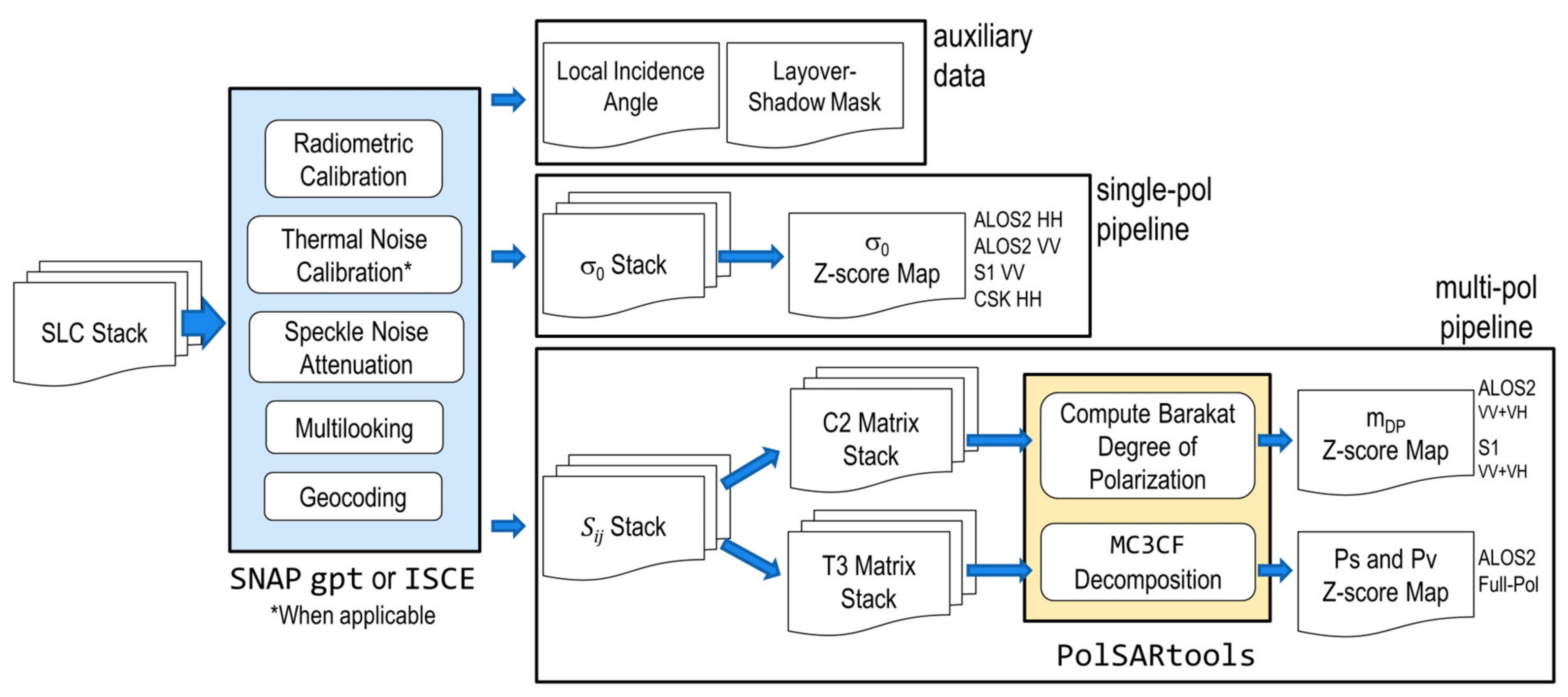
2.1. Single-Polarization: Backscattering Coefficient ()
Backscattering coefficient is the normalized measure of the radar signal’s strength reflected by a distributed target. From the single-look complex (SLC) stack, the general processing steps to obtain include radiometric calibration [26], speckle noise attenuation [27,28], multilooking and geocoding (Figure 1). For Sentinel-1 (S-1) data, thermal noise removal is carried out concurrently with radiometric calibration before converting the digital numbers to [29]. We only process the co-polarized stacks (HH or VV) for their higher sensitivity to surface-related scattering [30]. All data processing is carried out using the graph processing tool (gpt) in SeNtinel Application Platform (SNAP) and the InSAR Scientific Computing Environment (ISCE, for ALOS-2 ScanSAR data only) built in a high-performance computing cluster. Two auxiliary datasets, local incidence angle (LIA) and layover-shadow mask, are also generated during data processing [31]. LIA is the angle between the radar incidence direction and the slope normal vector. Small LIAs indicate slopes facing the satellite, while large LIAs indicate either slopes facing the satellite but significantly deviating from the line-of-sight (LOS) direction, or slopes facing away from the satellite.
2.2. Multi-Polarization: Degree of Polarization () and Scattering Powers
For a dual-polarimetric SAR data, we follow the same steps as those in the processing flow to generate geocoded complex scattering coefficients (Figure 1). We then construct the covariance matrix [32],
where indicates spatial ensemble averaging (using a 5 × 5 window in our case) and is the target vector,
From we can derive the 2D Barakat degree of polarization , which is defined as the ratio between the intensity of the polarized portion to that of the total intensity [33],
represents the anisotropy from polarization structures, whereas the scattering randomness, ( is a measure of the relative dominance of polarized scattering), is considered as the dual-pol radar vegetation index [34].
For the full-pol SAR data (ALOS-2 A122 in Table 1), we form the coherency matrix [30]:
where the target vector is defined as [30]
From , we carry out a Model-Free 3-Component decomposition for Full-pol data (MF3CF) which jointly considers the Barakat degree of polarization and the received wave information to allow the estimation of scattering powers without any assumption of scattering models [35]. The odd-bounce surface scattering power , even-bounce scattering power and the diffused (volumetric) scattering power can be estimated as [35]:
where is the 3D Barakat degree of polarization,
, and the scattering type parameter is defined as,
The calculation of 2D degree of polarization and scattering powers is carried out in PolSAR-tools available at https://github.com/Narayana-Rao/PolSAR-tools (accessed on 10 March 2022).
2.3. Generating Z-Score Maps
To standardize the change detection flow for various data values (, and scattering powers), we adopt a dimensionless Z-score (Z) of the post-event value normalized by the statistical information obtained from its pre-event time-series. It is calculated as [36],
where is the data value on the post-event epoch, and [, ] are the mean and standard deviation calculated from the pre-event time-series. The Z-score value represents the difference between a pixel’s change value and its background mean value in the unit of background standard deviations. The background mean and standard deviation are derived from multiple pre-event epochs, and therefore may avoid the issues associated with a single biased pre-event image, a consideration commonly seen in a dual-temporal change detection scheme [37]. It also allows a more robust detection of minor changes if the pre-event time-series contains relatively stable values [36].
Among different datatypes, however, we caution that the Z-score map for CSK data in the Hokkaido case (Table 1) may not be as accurate due to the insufficient number of pre-event images–no acquisition exists before 16 July 2017. The temporal standard deviations thus derived tend to be too large and yield Z-score values smaller than those generated from other datasets. To work around this problem, we estimate the spatial standard variation within a 21 × 21 window centered at each pixel, and use it as in Equation (9) when the value is smaller than the temporal standard deviation. The Z-score values thus generated are visually more comparable to other Z-score maps. The detection results, however, may still be less accurate because of incomplete pre-event information.
In addition to Z-score maps generated from the aforementioned datasets, we further generate a Z-score map that combines the positive Z-score values in () and negative values in (),
where stands for the combined Z-score map. The necessity and performance of such a combined Z-score map will be further demonstrated in Section 4. Next, we describe how these Z-score maps are used in the GSBA change-detection algorithm.
3. Change Detection Method
The method proposed in this study is a variation of the split-based approach (SBA), which was first proposed for SAR-based flood mapping [38]. SBA is designed for the generalization of a mapping algorithm regardless of the image’s spatial resolution, swath size and the target’s geospatial distribution. The basic idea is to separate the image into multiple, non-overlapping tiles (also called splits). The tiles are then checked one by one to identify the existence of a certain proxies that signify the changes. Some suggested proxies include standard deviation [38], coefficient of variation [39,40], and the ratio between the tile mean and the global mean [40]. Tiles with proxies above a given threshold are selected to jointly determine the global threshold either via a non-parametric approach such as the Otsu method [41] or the KI algorithm [42], or through a parameterized fitting to the data histogram in order to determine the best cutoff point [43,44].
One variation of SBA is the hierarchical split-based approach (HSBA) [45]. Different from the conventional SBA which adopts a uniform tile size [38,40,46,47], HSBA adaptively and hierarchically splits the image to variable sizes until a bimodal histogram (representing the change and non-change classes) can be identified in the tile or when a minimal tile size is reached. This way it avoids the need of a pre-defined tile size, which in some cases may compromise the detection if the change area within a tile is extremely large or small. The issue with HSBA is that the splitting process is nonlinear-every split depends on the result of the previous split, and hence the computation time can be long when the image is large.
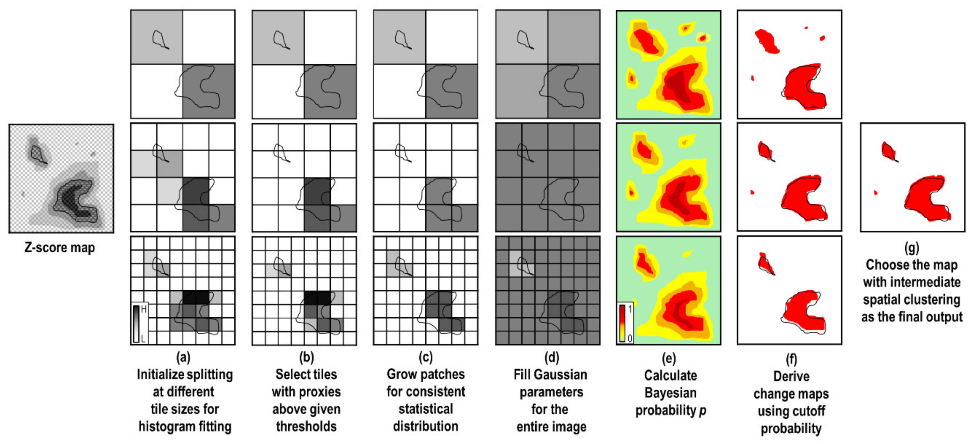
Instead of the top-down splitting strategy of HSBA, here we propose a bottom-up approach called Growing Split-Based Approach (GSBA) (Figure 2). We initialize the image splitting as in the conventional SBA. Once the tiles with changes are identified, we “grow” a patch within each tile cluster until the maximum patch area with a consistent bimodal histogram is reached. This growing step produces patches of different areas that mimic the variable tile size obtained by HSBA. The second variation in GSBA is that rather than obtaining a global threshold from the patches to generate a binary map, we calculate the Bayesian probability of changes instead [48]. Given the probability map, we can obtain a binary change map at a given cutoff probability (by default 0.5).
The last variation in GSBA is that instead of using a single tile size, the flow described above is repeated at different tile sizes. This practice is to acknowledge the observation that depending on the size and spatial distribution of changes, a single arbitrary tile size may in some cases produce results that fall into a local minimum or maximum of change area. With multiple binary maps generated at different tile sizes, we can select the one with intermediate spatial clustering (using Ripley’s K, see step (g) in Appendix A) as the final output. In other cases where different tile sizes produce similar binary maps, this practice also offers reassurance regarding the robustness of the detection output. The processing flow in GSBA is linear and can be fully parallelized, so the increase in computation time can be minor in a multi-processor computing system.
To avoid distraction from the main focus of this paper, details of the GSBA algorithm are given in the Appendix. The output Bayesian probability map is used in the following Receiver Operating Characteristics (ROC) curve analysis. To generate the ROC curves, we calculate the true positive rate (TPR, or recall) and false positive rate (FPR) at different cutoff probabilities. They are defined as follows:
where [T, F] stand for true and false, [P, N] stand for positive and negative, and any two-letter combination means the number of such pixels identified through validation. We further analyze the area under curve (AUC) to evaluate the overall detection performance. This continuous tracking of trade-off effects between TPR and FPR allows users to have a complete and visual overview of the detection performance [15]. To compare with other studies using the same landslide cases, we also report the overall accuracy (OA) by using the final binary maps from GSBA. The overall accuracy is defined as:
OA = (TP + TN)/(TP + TN + FP + FN)
Note that these metrics are calculated at each datatype’s spatial resolutions, which means, the validation dataset is resampled to match the resolution of the SAR images.
4. Results
4.1. Case Study 1: Earthquake-Triggered Hokkaido Landslides in Japan
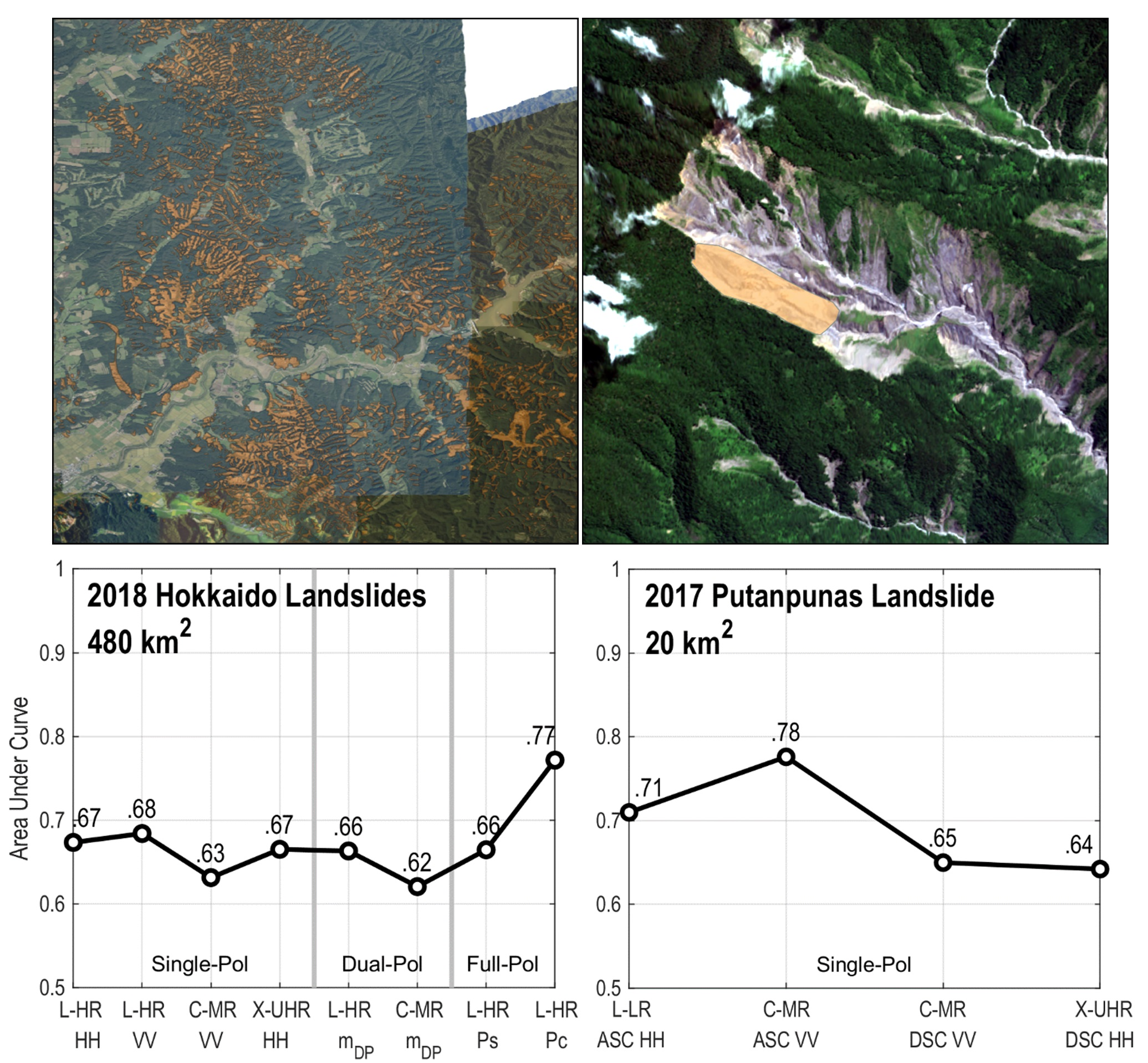
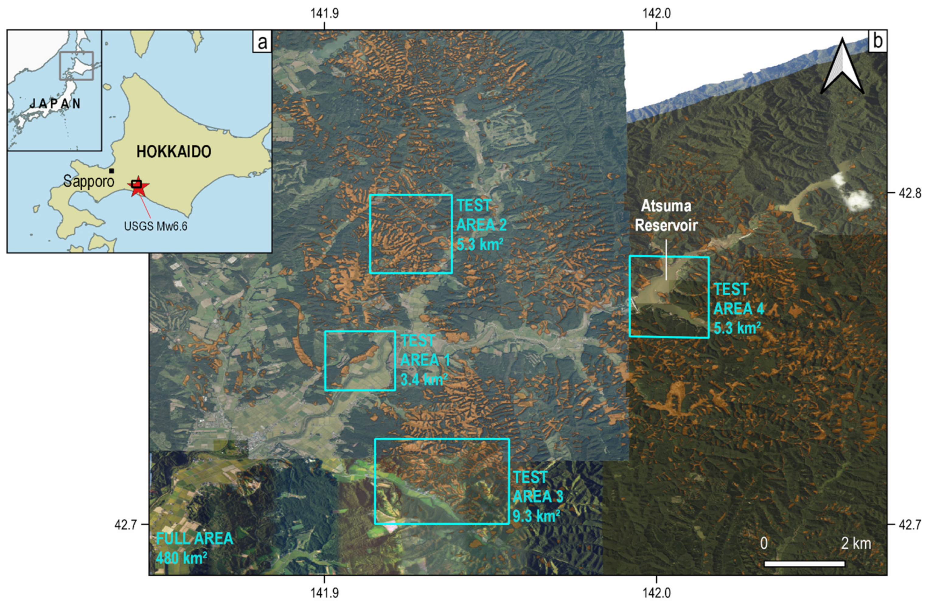
Widely-distributed landslides occurred due to seismic shaking during the 6 September 2018 Mw 6.6 Hokkaido Eastern Iburi Earthquake (Figure 3). After the earthquake, the Geospatial Information Authority of Japan (GSI) acquired aerial photos on 6 and 11 September over the landslide areas and identified more than 3300 landslide patches manually (https://www.gsi.go.jp/BOUSAI/H30-hokkaidoiburi-east-earthquake-index.html#1, accessed on 10 March 2022). Visual comparison between the aerial photos taken on 6 and 11 September shows that only minor changes occurred between these two dates, and hence the majority of the landslides have existed since the earthquake.
We define a large area of interest (AOI) of 480 km2 that covers most of the landslide patches (Figure 3). Within the large AOI we further define four test areas, three of which are the same as those chosen by Jung and Yun (2020) [15]. This choice allows us to compare the effect of different spatial resolutions-they adopt the ALOS-2 PALSAR-2 Ultra-Fine HH-pol SAR data of 3-m resolution, while the data used in this study is the 6-m High-Sensitive full-pol SAR. In addition, we define a fourth test area around the Atsuma Reservoir in order to examine the effect of water bodies during landslide detection.
4.1.1. Qualitative Comparison
From the three sensors used in this case study (Table 1), we produce the following seven SAR datatypes and one combined Z-score map to carry out the performance comparison:
- (1)
- High-res L-band HH-pol
- (2)
- High-res L-band VV-pol
- (3)
- Medium-res C-band VV-pol
- (4)
- Ultra-high-res X-band HH-pol
- (5)
- High-res L-band dual-pol (VV + VH)
- (6)
- Medium-res C-band dual-pol (VV + VH)
- (7)
- High-res L-band full-pol
- (8)
- High-res L-band full-pol (denoted as datatype hereafter)
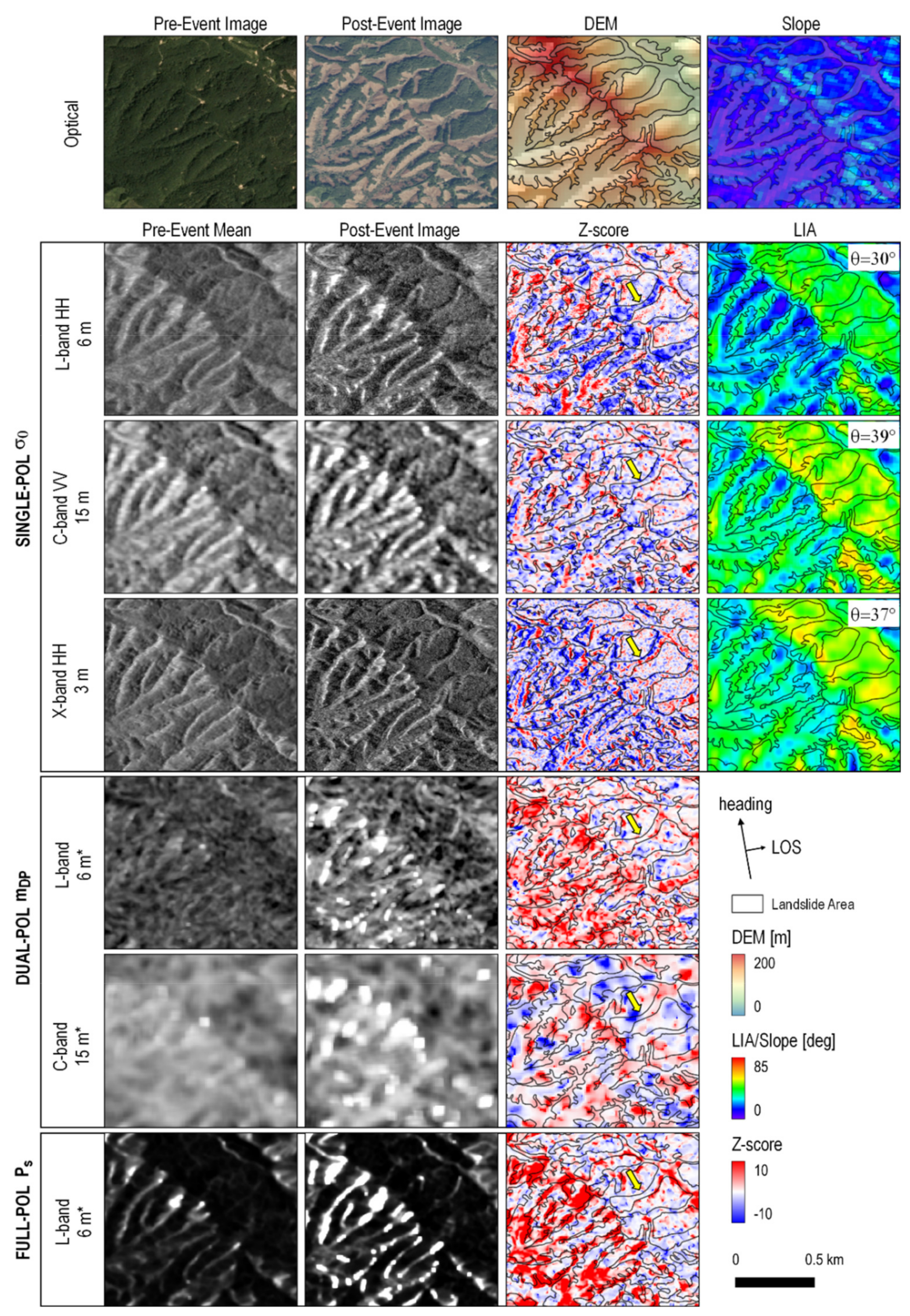
In Figure 4 we choose Test Area 2 to demonstrate the differences among some of the selected datatypes. Both the high-res L-band HH-pol and the ultra-high-res X-band HH-pol provide sharp outlines for landslides compared to the multi-pol datatypes ( and ). This difference is caused by the spatial ensemble averaging carried out on the polarimetric datasets. The C-band VV-pol , acquired at a lower spatial resolution, does not capture the landslide boundaries as clearly. In addition, many pixels in the landslide patches contain low Z-score values, suggesting that these pixels are indistinguishable from non-landslides. The same phenomenon is also observed more in the X-band than in the L-band , implying that shorter radar wavelengths may not perform as efficient in landslide detection within forest areas, possibly due to their higher sensitivity to small-scale changes in vegetation during the pre-event periods.
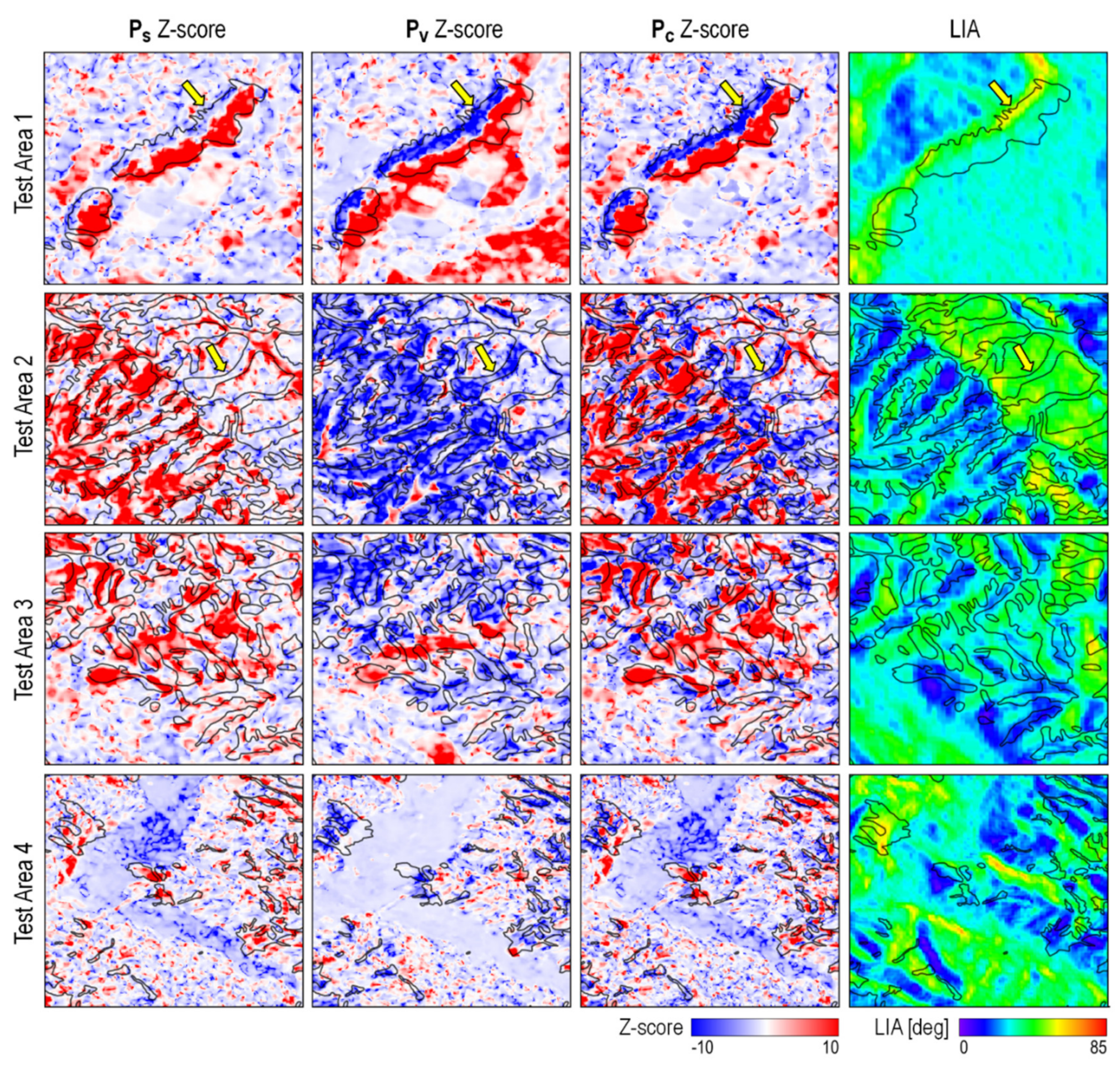
Next, we examine the effect of viewing geometry on different polarimetric combinations in the L-band datatypes. The datatype shows strong positive Z-scores for the landslides on the slopes with small LIAs. On the slopes with large LIAs, the landslide patches contain low to nearly zero Z-scores (pointed by yellow arrows in Figure 4). The same is also seen on the Z-score map. In comparison, the L-band may still show clear and predominantly negative Z-score values on the slopes with large LIAs. We investigate the Z-score maps from other scattering powers and find that, instead of a positive increase in Z-score, landslide patches with larger LIAs tend to show a stronger decrease in Z-score (yellow arrows in Figure 5). This different dependency on LIA between and is also observed in other landslide cases [23]. Numerical simulation in [49] offers some possible explanation to this phenomenon, in which backscattering energy due to direct-ground reflection and crown-ground interaction decreases with LIA, while the energy due to direct-crown backscattering increases. In other words, landslides on the slopes with larger LIAs are sensed as “loses in tree crowns” instead of “increases in bare surfaces”. That means or each only carries half of the information about landslides. It is therefore necessary to consider both values when carrying out landslide detection, such as by combining them into a joint Z-score map (Equation (10) and Figure 5).
The aforementioned complementary effect between or is not seen between the dual-pol and the dual-pol radar vegetation index [34]. In fact, when comparing the Z-score maps generated from these dual-pol parameters, one appears as a sign-flipped image of the other–pixels in the landslide patches display similar amplitudes but opposite signs on the two Z-score maps. This is probably due to the incomplete information of scattering properties in dual polarization. We therefore do not attempt to combine these two parameters and remain with the -only Z-score map. Next we will look into the quantitative comparison of detection performance among the eight listed datatypes.
4.1.2. Quantitative Comparison
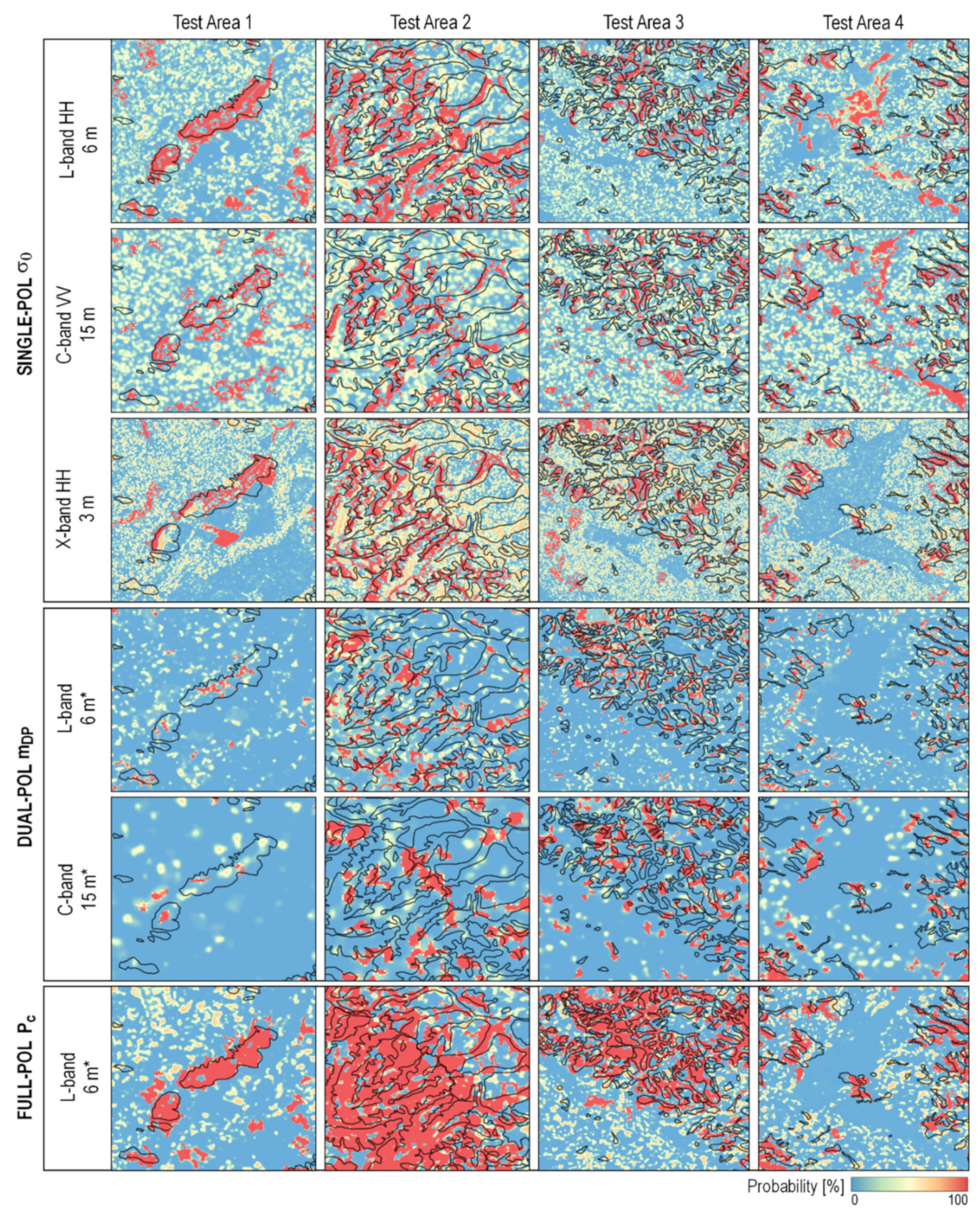
Figure 6 shows the Bayesian probability maps calculated from different datatypes. Overall, the full-pol depicts the most complete shape of the landslide bodies, followed by the single-pol at different radar wavelengths. The dual-pol datatypes detect only few landslides. The X-band captures an additional high-probability patch in Test Area 1 with sharp outlines. This patch is possibly related to crops, and the false detection is likely associated with the lower number of pre-event images. In areas where water bodies exist (Test Area 4), the single-pol may detect changes associated with both the landslides and the water bodies, while the multi-pol datatypes are relatively free of such confusions.
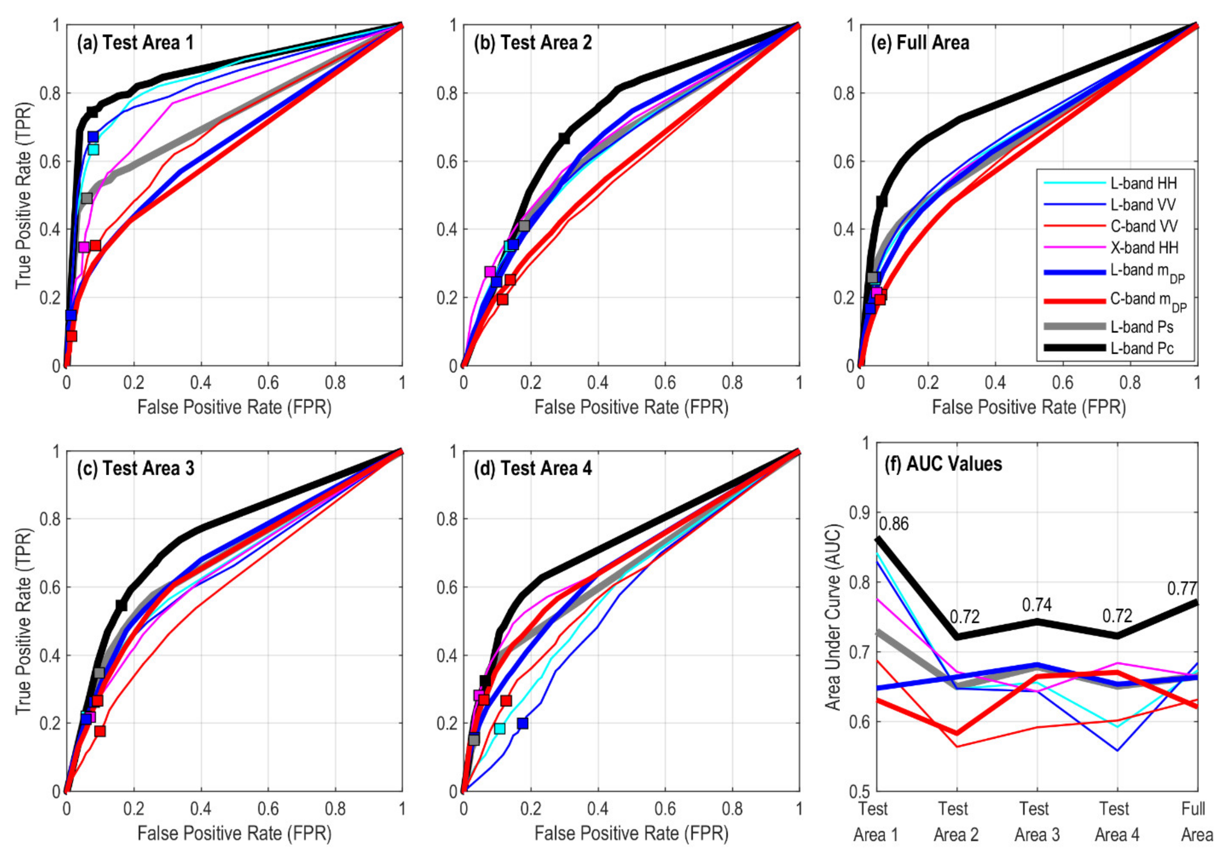
The performance of each datatype is shown in the ROC curves (Figure 7). In Test Area 1, the ROC curves for the L-band and show a steep increase of TPR at low FPR, yielding AUC values as high as 0.83 to 0.86 (Figure 7f). These values are comparable to the detection results based on the ALOS-2 Ultra-Fine HH-pol multi-temporal intensities of 3-m spatial resolution (AUC = 0.79) [15]. The AUC for X-band and L-band rank the second and third at 0.77 and 0.73. The L-band , C-band and C-band perform poorly, yielding AUC values lower than 0.7.
The landslide patches in Test Area 2, 3 and 4 result in slow-rising ROC curves and low AUC values in almost all datatypes (Figure 7b–d,f). Among them, the full-pol still gives the highest and more stable AUC values, above 0.7 for all three test areas. All the other datatypes yield AUC values lower than 0.7. The C-band yields the lowest AUC in Test Area 2 and 3–lower than 0.6. In Test Area 4, the L-band gives the lowest AUC values as a result of false detection over the reservoir lake (Figure 3 and Figure 6).
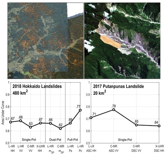
For the full area, the L-band full-pol has superior performance in landslide detection with AUC = 0.77 (Figure 7f). The comparison between and -only AUC values again confirms that the combination of and is necessary for landslide detection. The full-area AUC value for the high-res L-band and ultra-high-res X-band ranks the second and third, higher than the medium-res C-band . We can therefore confirm that spatial resolutions plays a role as important as radar wavelengths in SAR-based landslide detection. The performance of the dual-pol is least favored because of its lower full-area AUC and its tendency to detect fewer landslides.
In Figure 7a–e, we also mark the positions of the binary change maps determined by GSBA on each ROC curve. These solutions are located close to the turning points of the curves, but slightly leaning towards the lower-FPR end. These positions suggest that the default cutoff probability of 0.5 tends to create conservative change maps with a higher positive likelihood ratio (TPR-to-FPR ratio).
4.2. Case Study 2: Rainfall-Triggered Putanpunas Landslide in Southern Taiwan
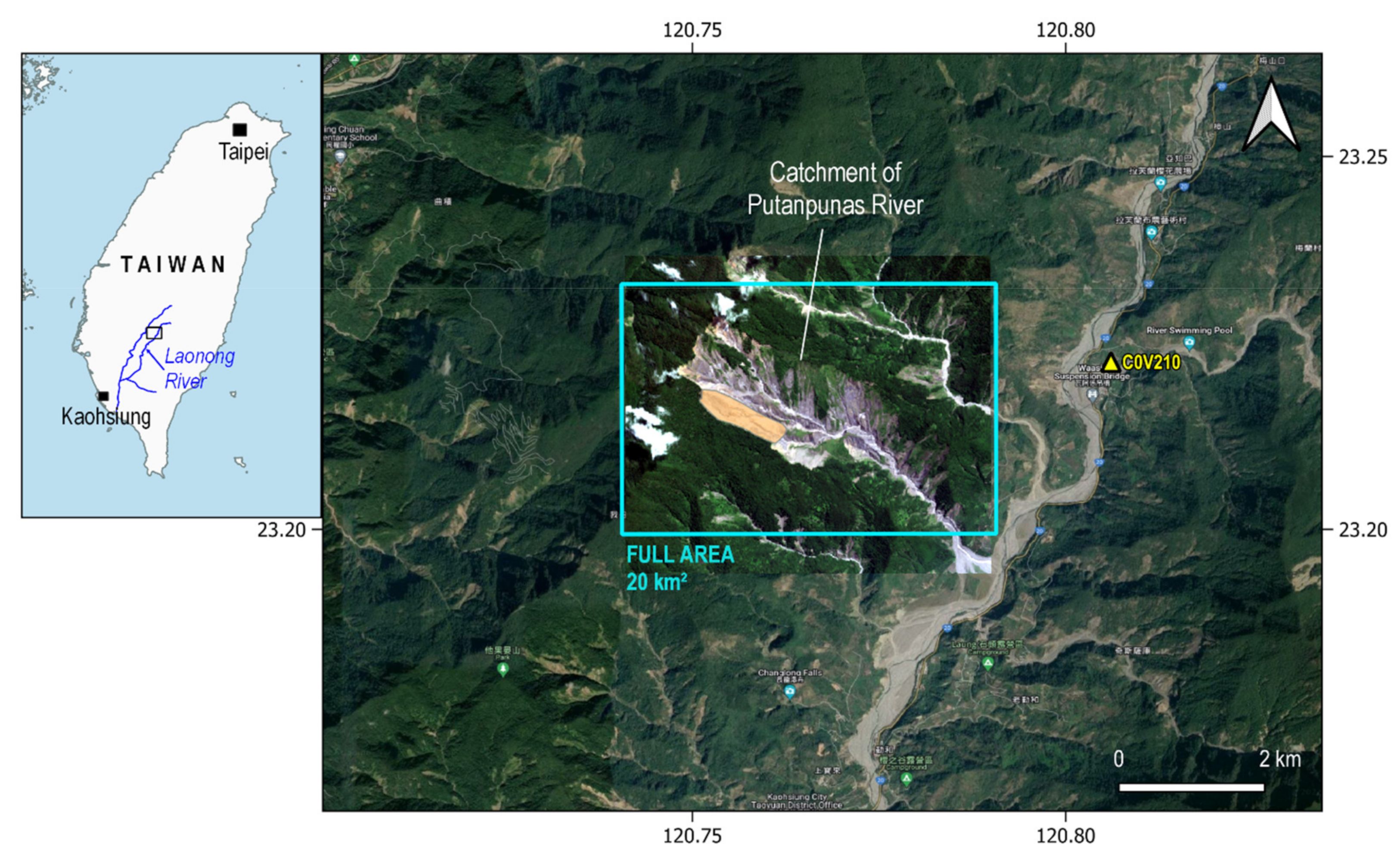
In the second case, we look into a different scenario–a rainfall-triggered landslide. During the first 4 days in June 2017, a total of nearly 900 mm of precipitation occurred in the upstream of the Laonong River (according to the records from weather station C0V210, available at https://e-service.cwb.gov.tw/HistoryDataQuery/index.jsp, accessed on 10 March 2022) (Figure 8). Three days later on 7 June 2017, a landslide-associated earthquake (landquake) was detected through the Real-time Landquake Monitoring System (RLAMS, http://collab.cv.nctu.edu.tw/older/catalog_20171231.html, accessed on 10 March 2022) [50]. Given the order of occurrence between the torrential rain and the landquake, we attribute this event to a rainfall-triggered landslide.
To determine the landslide area associated with the 7 June 2017 landquake, we use SPOT-6/7 images acquired on 18 April 2017 and 5 July 2017 to carry out manual detection. Within a 15-km radius (approximately the estimation error of landquake relocation) of the epicenter, we locate a new sliding patch in the existing landslide area of the Putanpunas River catchment. Actually, there have been repeating landslides in this catchment since typhoon Morakot in the year of 2009 [18,51], making this catchment one of the most actively evolving landslide area in southern Taiwan. Different from the multiple small-scale landslides triggered by the Hokkaido Eastern Iburi Earthquake, this rainfall-triggered Putanpunas landslide contains a single patch of a relatively large area, up to 400,000 m2 (Figure 8). We caution that the actual landslide patch may differ from what we map here due to the longer latency between the event date and the post-event optical image.
4.2.1. Qualitative Comparison
In this case study, we produce the following five datatypes for comparison (note that different viewing geometry is involved):
- (1)
- Low-res L-band HH-pol , ascending
- (2)
- Low-res L-band HH-pol , descending
- (3)
- Medium-res C-band VV-pol , ascending
- (4
- Medium-res C-band VV-pol , descending
- (5)
- Ultra-high-res X-band, HH-pol , descending
Some datasets allow dual-pol polarimetric combinations, such as HH-HV for ALOS-2 track D27 and VV-VH for both Sentinel-1 tracks (Table 1). However, in the Hokkaido case we have demonstrated that the use of dual-pol datatype tends to capture fewer landslides, so we decide not to adopt the dual-pol datatype in this case study. Here we wish to focus on the detection performance among the datatypes of different wavelengths, spatial resolutions and viewing geometry.
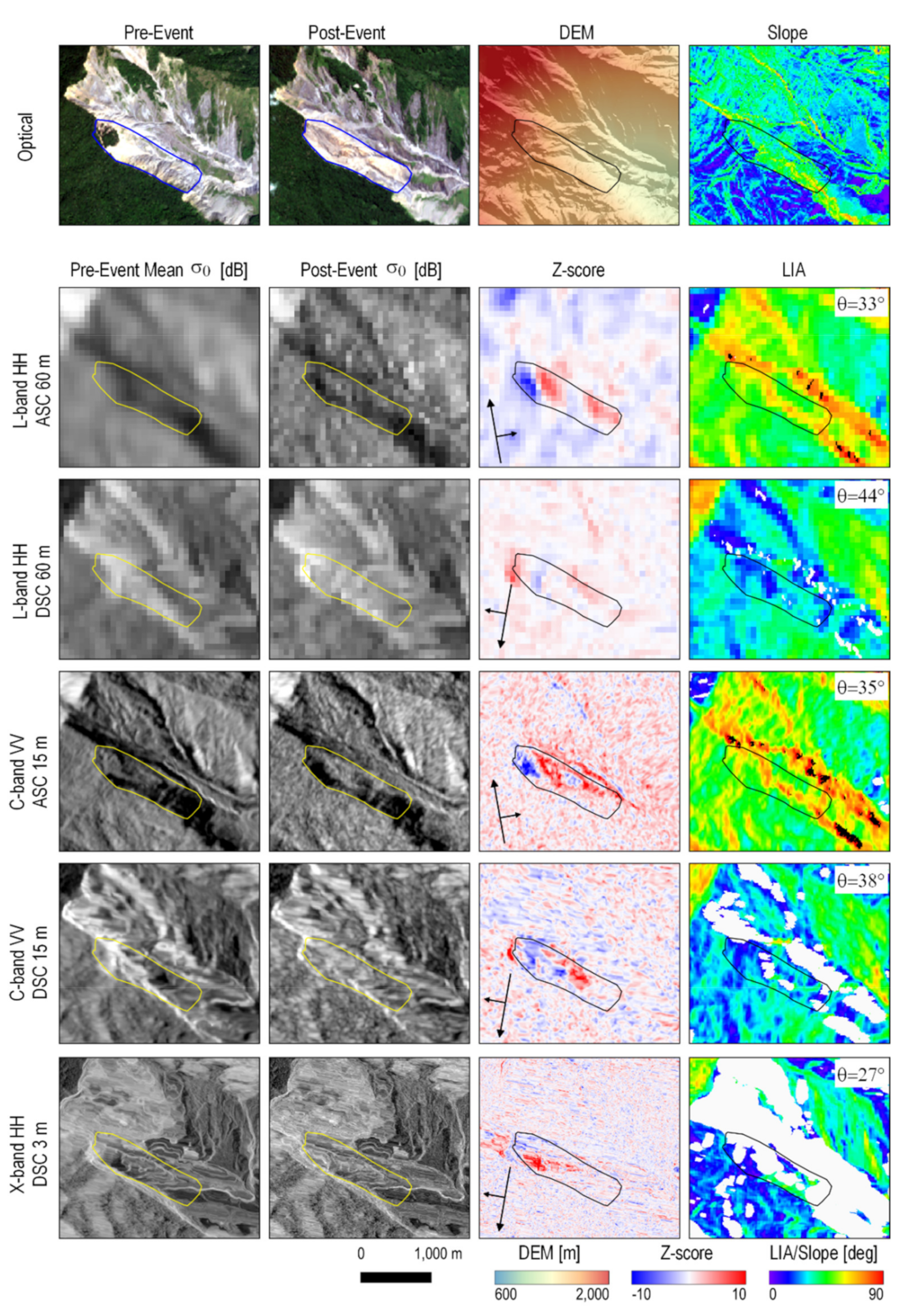
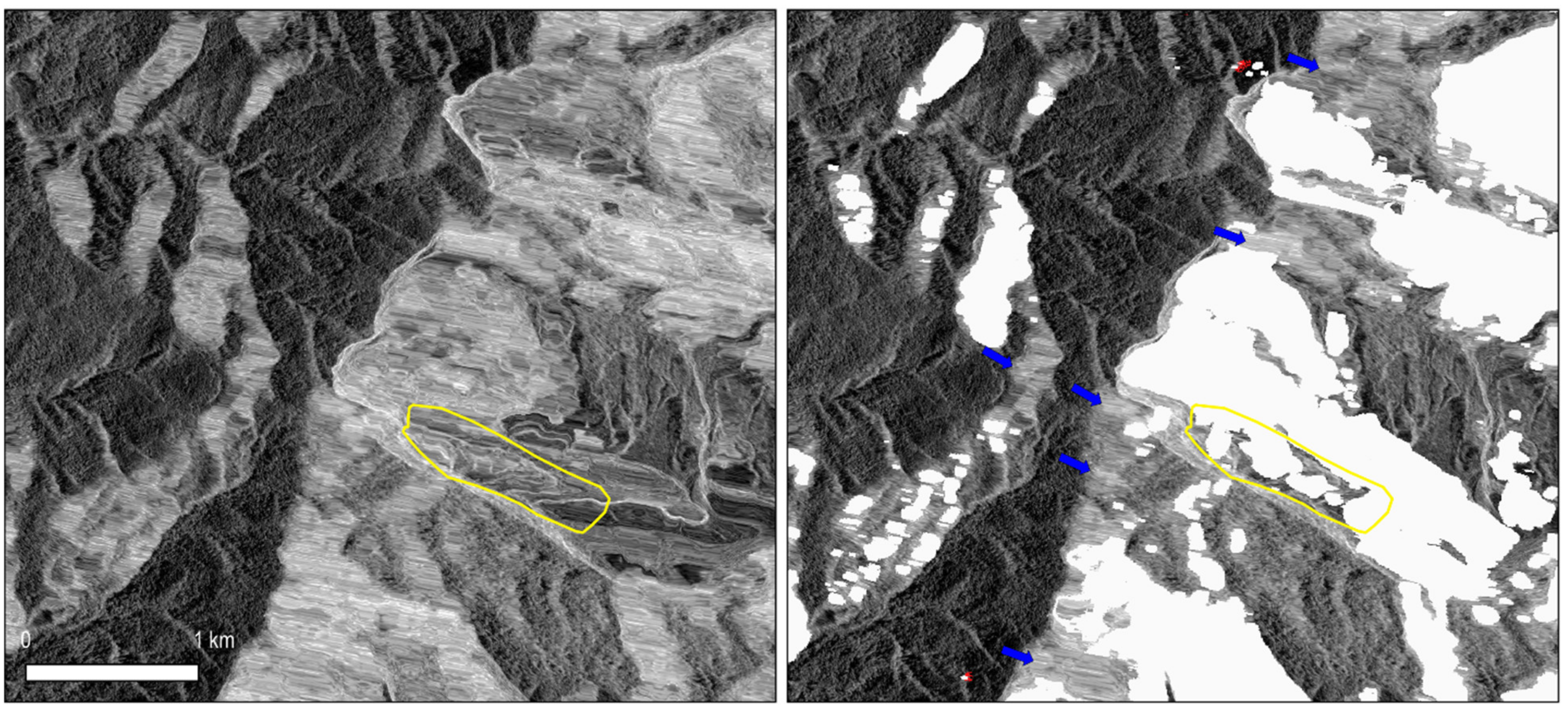
Figure 9 shows how different datatypes compare visually. The ascending tracks show more prominent landslide signatures on the Z-score maps compared to those from the descending tracks, regardless of the wavelengths and spatial resolutions. The intriguing point is that the viewing geometry from ascending tracks yield larger LIAs compared to those from descending tracks. In addition, we find that the viewing geometry from descending tracks produces large layover zones that tend to overlap with the slopes of small LIAs. Among all sensors, the X-band CSK descending track produces the largest layover area, which also corresponds to the smallest look angle (27°) among all three sensors. Within the layover zones, landslide-related changes may still be recorded but are mixed with energies from multiple ground targets of the same range distance, leading to brighter pixels and stretched patterns after geocoding (Figure 10). We also notice that the current layover-shadow mask does not necessarily mask out all layover areas (Figure 10), which is possibly caused by errors in DEM or limitations in the SAR geometric distortion simulation [52].
We have to emphasize that the same layover-shadow masks are also calculated and applied on the SAR images in the previous Hokkaido landslide case. However, given the smaller slope angles (Figure 4), the layover and shadow effects are nearly negligible. In comparison, the Putanpunas River catchment has a large topographic relief and hence greater slope angles (Figure 9), resulting in a larger portion of unusable data within the layover zone.
4.2.2. Quantitative Comparison
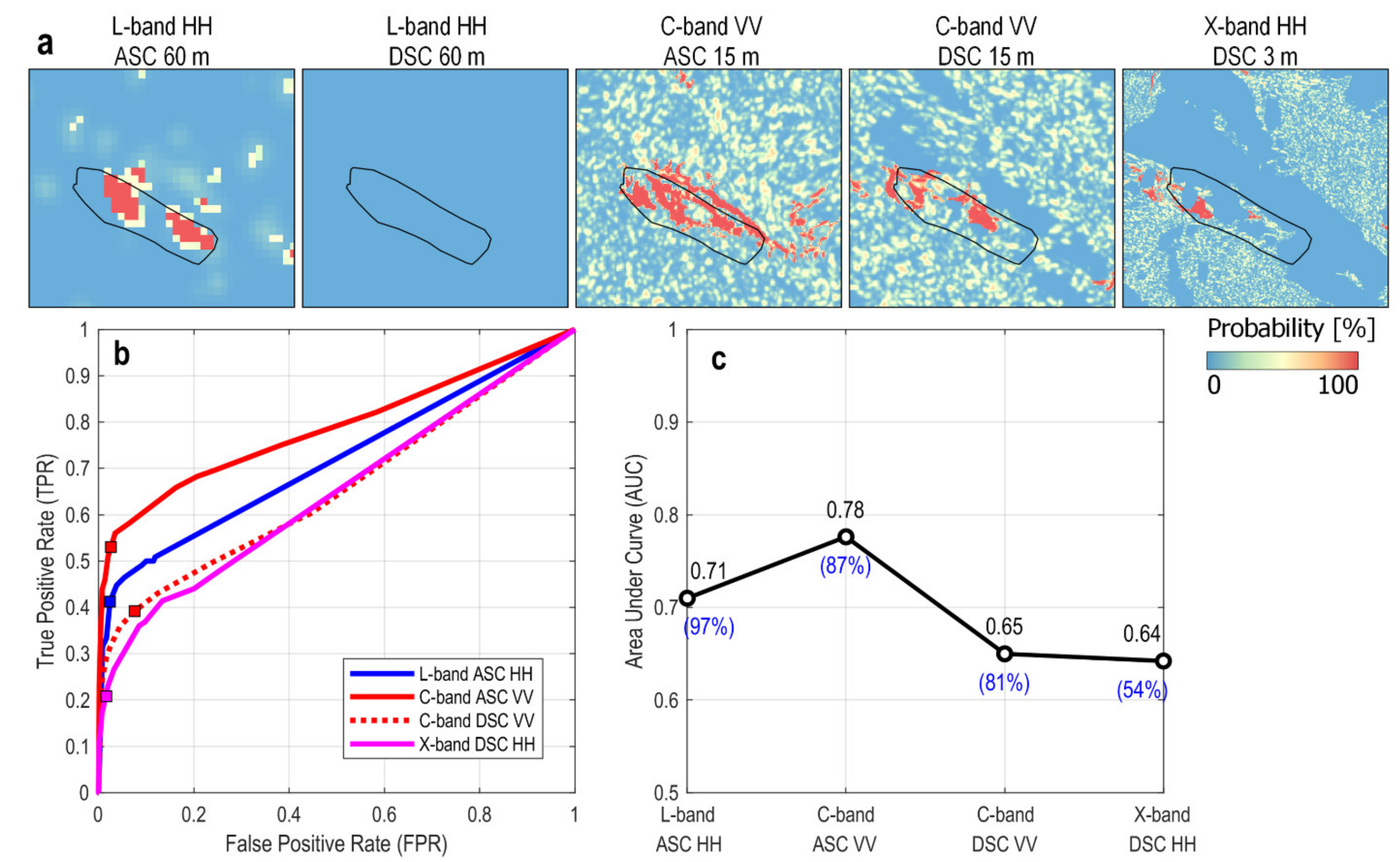
Figure 11 shows the Bayesian probability, ROC curves and AUC values for different datatypes. The ascending tracks show better performance than descending tracks, with the highest AUC of 0.78 from the medium-res C-band VV . The ascending L-band HH , albeit its low spatial resolution (60 m), still yields an AUC value of 0.71. On the other hand, the descending tracks do not detect as many changes, with an AUC value of 0.65 for the medium-res C-band VV and 0.64 for the ultra-high-res X-band HH . No change is detected from the descending L-band HH . We should point out that despite the similar AUC values from the descending C-band VV and the X-band HH , their effective area (unmasked area) is different–more than 50% of the catchment is under the layover-shadow mask of the X-band data.
5. Discussion
5.1. How Data Properties Affect Detection Performance
In Table 2 we summarize the performance of different datatypes, including the full-area AUC and OA. Note that AUC does not represent the performance of any particular detection outcome but a full spectrum of outcomes, whereas OA is calculated at a specific selection (e.g., at the cutoff probability of 0.5) to mimic the operator’s choice. The OA values among different datatypes in the Hokkaido case, however, are all very similar and cannot reflect their actual relative performance. This similarity results from the large number of non-landslide pixels (TN in Equation (12)) when computing the OA values. To allow a better judgement of the relative performance at a specific landslide mapping outcome, we compute the full-area TPR at a fixed FPR of 0.1 (TPRFPR = 0.1). This value indicates the ratio of detectable landslides at the cost of 10% false positive detection. In the Hokkaido case, we further normalize the TPRFPR = 0.1 values by using the best TPRFPR = 0.1 from (Table 2). With the AUC and TPRFPR = 0.1 values, we discuss how the following data properties affect the performance of SAR-based landslide detection.
Radar wavelengths and spatial resolutions. In the Hokkaido case, the L-band datatypes have better AUC and TPRFPR = 0.1 values than the other two radar wavelengths. This result seems to suggest that longer wavelengths work better in landslide detection. However, spatial resolutions can be an equally important factor. This inference is made from the poor performance of the medium-res C-band single-pol datatype–its result is worse than that from the X-band single-pol data at a higher spatial resolution. At the same time, the medium-res C-band single-pol data seems to perform relatively well in the Putanpunas case. This better performance is probably associated with the geometry of the landslide patches (small and distributed landslides in Hokkaido vs. one single large patch in Putanpunas), and the fact that the Putanpunas landslide is a repeated landslide on a bare surface instead of on a forested land (Figure 8).
Polarizations. In the Hokkaido case, the high-res L-band full-pol data can offer the best landslide detection capability in forest areas. It can even avoid false detection over water bodies. Even though the landslide boundaries become slightly blurry compared to those detected by using single-pol datatypes, the amount of information contained in a full-pol dataset and the detection performance thereof is indeed unparalleled. The L-band dual-pol datatype, despite a slightly better TPRFPR = 0.1, gives an AUC value lower than those from many single-pol datatypes. It also tends to detect fewer landslide patches. As dual polarization will be a major observation mode for some upcoming missions such as NISAR, more efforts are needed to explore a better utilization strategy for dual-pol data in landslide mapping.
Viewing Geometry. In the Hokkaido case, we do not see a notable difference in LIA between the detected and the missed pixels (Figure 12a). This similarity in LIA distributions suggests that large LIAs do not necessarily hinder landslide detection. In the Putanpunas case, landslides are even better detected on datatypes with larger LIAs (Figure 9). On the other hand, slopes with small LIAs may coincide with overlay zones, which are also seen in the Putanpunas case. The smaller (steeper) the satellite look angle (θ), the larger the overlay zone and the smaller the effective area. The percentage of effective area drops from 97% at θ = 44° (ALOS-2 D27) to 54% at θ = 27° (CSK-D) (Figure 9 and Table 2). As the area of layover and shadow depends on the specific topography of a region, a DEM-based SAR geometric distortion simulation should be executed before planning for a mission or submitting a tasking request in order to determine the best viewing geometry [52].
5.2. Limitations in SAR-Based Landslide Detection
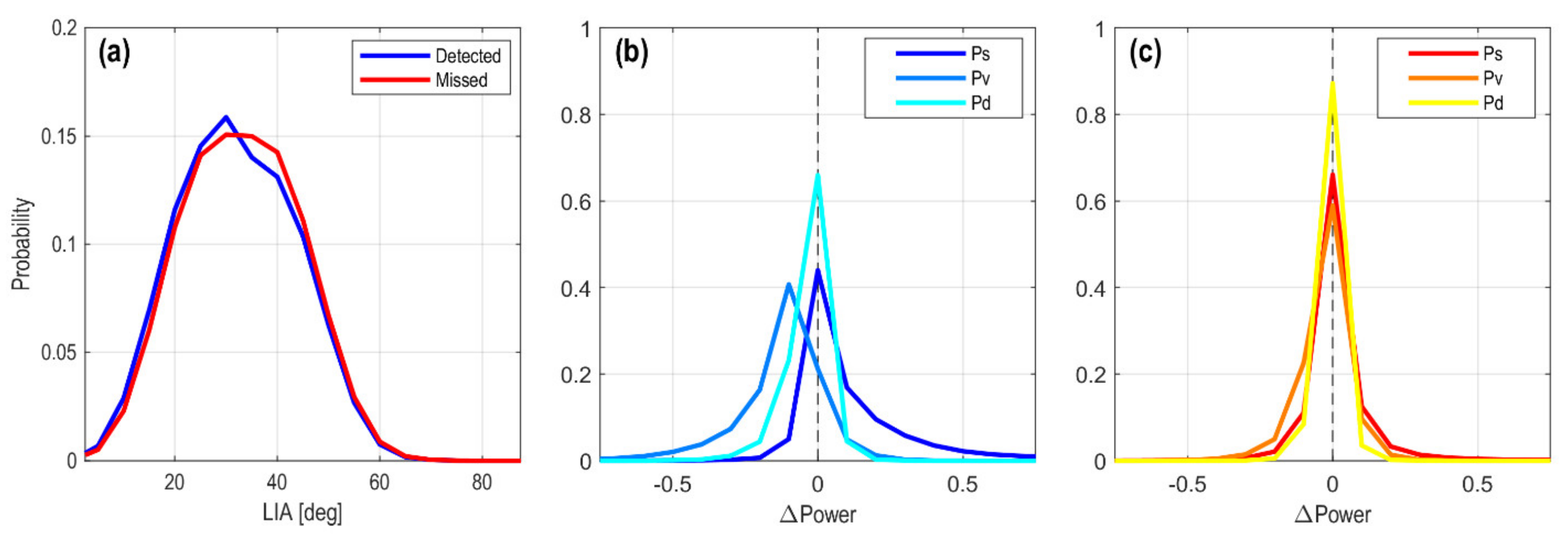
In the Hokkaido case, the best full-area AUC is 0.77 and the best OA is 0.90 (Table 2). These values are close to the results produced by using the ultra-high-res L-band HH-pol multi-temporal intensity with different detection algorithms [15]. The similarity in limited performance from different studies suggests that there may exist some factors that prevent the SAR-based landslide mapping from achieving the high accuracy attained in optical image-based mapping [53]. We plot the histogram of the post-to-pre-event difference in scattering powers () for the detected and the missed pixels, respectively, within the Hokkaido AOI (Figure 12b,c). While the histograms for the detected pixels are clearly skewed, the histograms for the missed pixels are centered and symmetric around zero, indicating no significant difference in any of the scattering powers before and after the landslide. This phenomenon is bewildering and needs some explanation.
The first possibility is the change of local topography. From a broader scale, there does not seem to be a systematic difference in LIA between the detected and the missed pixels (Figure 12a). However, the LIA is calculated using the pre-event global 30-m DEM [54]. The topography must have changed locally after the landslide. In fact, according to the post-event DEM obtained by airborne laser survey, the surface morphology within the landslide patches has changed substantially [55]. Features such as scarps and crown cracks can reach meters tall with very steep (nearly vertical) facets [55]. Field photos also reveal that large boulders, huge piles of dead trees and meter-scale surface undulations exist on the ground [55,56]. The chaotic distribution of these features may result in scattering properties considerably deviating from what is expected from a pure land cover-type change (forest to bare surface).
Another equally important factor to consider is the spatial variation of water contents. Several studies show that the water contents can vary remarkably in the Hokkaido area, from 30% to 280% among different geological materials sampled at the same site [57,58]. As these materials are spread out during the landslide, the randomness in surface soil moisture within the landslide patches increases. To sum up, soil moistures, local topography, surface roughness and land cover changes together form a complicated backscattering field in the landslide patches, leading to clear changes of scattering powers in some places and no clear changes in other places. We may even hypothesize that it is radar wave’s sensitivity to multiple physical properties that limits its performance in landslide detection. This hypothesis needs further validations though, such as through numerical simulation of 3D backscattering fields.
The increased randomness in backscattering fields within a landslide patch may explain why intensity correlation method can yield better detection results than those from pixel-by-pixel detection methods [15,19]. Intensity correlation is calculated based on a number of pixels within a moving window, which offers contextual information about the objects and their changes. Most important of all, it can potentially average out the randomness in the complicated scattering field within a landslide patch, leading to a smoother and less noisy detection result.
6. Conclusions
By applying a newly-designed change detection algorithm Growing Split-Based Approach (GSBA) on two different landslide cases, this study examines how different SAR data properties affect the performance of landslide detection. Our result shows that the high-resolution, full-polarimetric SAR datatype has unparalleled performance in landslide detection over forest areas. Single polarimetric datasets of high or ultra-high spatial resolution rank the next, regardless of their radar wavelengths. This result suggests that high spatial resolution is critical especially for detecting small and distributed landslides in forest areas. Datatypes of medium or low spatial resolution work better in detecting large landslide patches over bare surfaces; their detection performance decays significantly over small landslides in forest areas. Dual polarimetric datatypes have the worst performance among all; a better utilization strategy may be needed for their use in landslide detection. Different viewing geometry mainly impacts the effective detection area by creating layover and shadow zones. This problem is more severe in areas of large slopes (≥40–50°), in which a steep viewing angle (<30°) may render half of the image unusable for landslide detection. SAR geometric distortion simulation is recommended before planning for a mission or submitting a tasking request for landslide mapping purposes. Given the limited performance of SAR-based landslide detection (both in this study and in previous studies) as compared to that from optical image-based landslide detection, we propose that other confounding factors, including but not limited to local topography, surface roughness and soil moistures, are all contributing to the randomness in the backscattering field and hinder the detection of land cover changes. Such limitations need to be properly acknowledged when adopting SAR-based landslide mapping for emergency responses or post-hazard assessments.
Author Contributions
Conceptualization, Y.N.L.; data curation, Y.-C.C., Y.-T.K. and W.-A.C.; formal analysis, Y.N.L.; methodology, Y.N.L. and Y.-C.C.; project administration, Y.N.L.; software, Y.N.L. and Y.-C.C.; validation, Y.-C.C. and Y.-T.K.; writing—original draft, Y.N.L. and Y.-C.C.; writing—review and editing, Y.-T.K. and W.-A.C. All authors have read and agreed to the published version of the manuscript.
Funding
This research was supported by research grant AS-TP-108-M08-1 from Academia Sinica, Taiwan and MOST 110-2119-M-001-006 from the Ministry of Science and Technology, Taiwan to Y.N.L.
Data Availability Statement
ALOS-2 data between 2016 and 2018 used in this study are provided by JAXA via the EO-RA2 research program (PI number: ER2A2N006). Copernicus Sentinel data between 2016 and 2018 used in this study are processed by ESA and retrieved from ASF DAAC. The COSMO-SkyMed data are purchased from e-GEOS. The airborne optical images for the Hokkaido landslides are available through the Geospatial Information Authority of Japan.
Acknowledgments
We thank Hsin Tung for handling the COSMO-SkyMed dataset. We also thank two anonymous reviewers for their constructive suggestions which improve the quality of this paper. This work is IES paper number 2408.
Conflicts of Interest
The authors declare no conflict of interest.
Appendix A. GSBA Algorithm
The following description corresponds to the steps illustrated in Figure 2.
- (a)
- Initialize splitting and histogram fitting
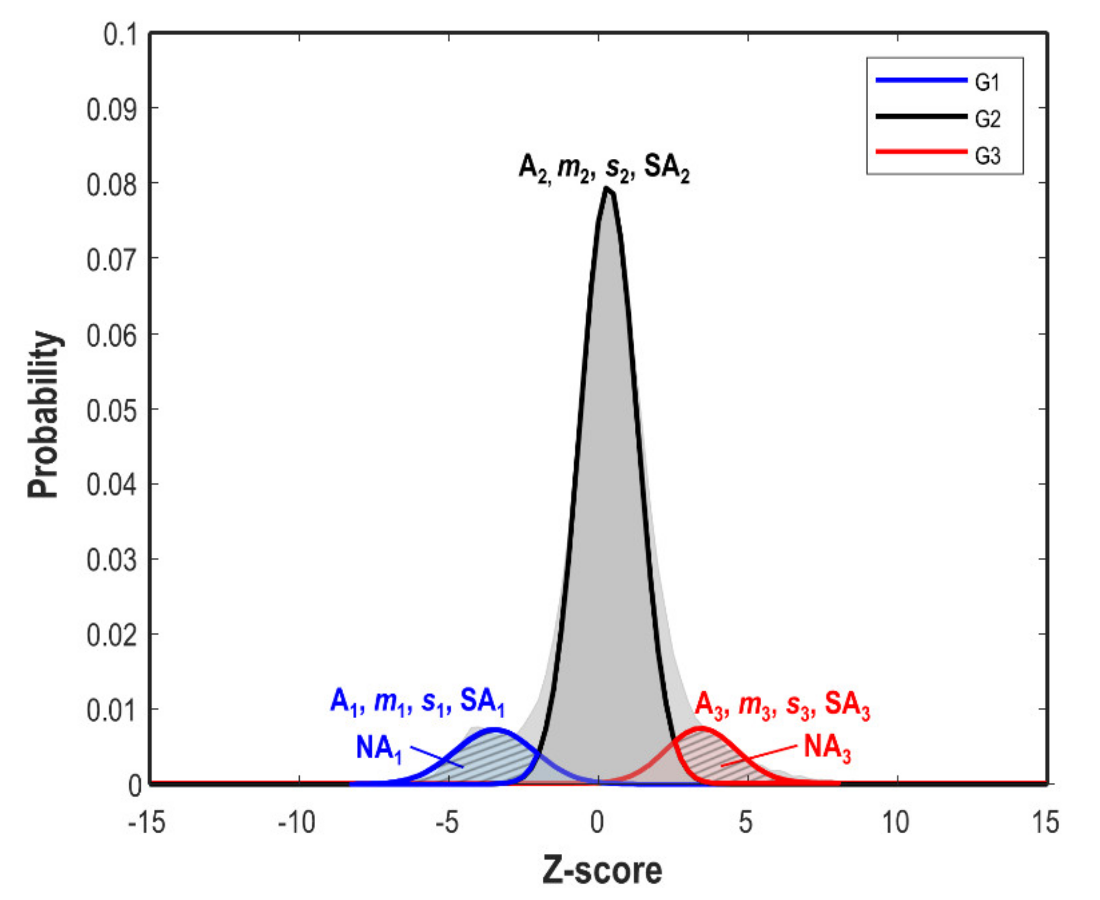
We first split the image into multiple tiles. After splitting, we fit the data histogram within each tile with a model histogram of tri-modal Gaussian distribution (modified after the bimodal Gaussian distribution in [48]):
where is the modeled histogram discretized at bin centers, [] is the amplitude, mean and standard deviation for each of the i-th Gaussian modes. Mode 1 () and mode 3 () imply negative and positive changes in Z-score values, respectively. Mode 2 () has a mean value close to zero for the unchanged class (Figure A1). In the rest of this paper, we use Gaussian parameters to refer to [] for the three modes. The curve-fitting optimization is carried out by using the fast nonlinear solver of the Levenberg-Marquardt algorithm [59].
Figure A1.
Tri-model Gaussian distribution. Mode 1 () and Mode 3 () are for the changes with decreased and increased Z-score values, whereas Mode 2 () is for the unchanged class. SA is surface area under the colored curve. NA is the non-overlapping area, marked by slash stripes.
Figure A1.
Tri-model Gaussian distribution. Mode 1 () and Mode 3 () are for the changes with decreased and increased Z-score values, whereas Mode 2 () is for the unchanged class. SA is surface area under the colored curve. NA is the non-overlapping area, marked by slash stripes.

- (b)
- Select tiles using thresholds
The tiles are selected based on the following proxies:
- i.
- Ashman D coefficient (AD). It represents the separation between two modes. The value is defined as [60]:
- ii.
- Bhattacharyya coefficient (BC). It represents the goodness of fit in terms of probability. It is defined as [61]:where stands for the -th histogram bin.
- iii.
- iv.
- Non-overlapping Ratio (NR). It represents the significance of the changes in terms of the cumulative probability that is not overlapped with the unchanged class (). It is defined as:
The first three proxies are also used by HSBA [45], while the last one (NR) is an additional proxy implemented in GSBA. The main purpose of NR is to weed out the tiles where the mode has a wide distribution that overlap significantly with the other two modes. Except for BC, the other three proxies are calculated for (i = 1) and (i = 3) mode separately. Table A1 shows the empirical tile selection thresholds used for landslide selection in this study.

Table A1.
Tile selection thresholds for landslide detection.
| Ashman D Coeff. () | >1.9 |
| Bhattacharyya Coeff. () | >0.98 |
| Surface Ratio () | >0.05 |
| Non-overlapping Ratio () | >0.4 |
- (c)
- Grow patches for consistent statistical distribution
Next we try to merge the tiles in order to obtain more robust Gaussian parameters from clustered changes. Within each tile cluster, GSBA first chooses a random seed tile and identifies the neighboring tiles around it. The first round of histogram fitting (Equation (A1)) is carried out on the joint histogram between the seed and each of the neighboring tiles. The neighboring tiles with proxies above the thresholds shown in Table A1 are selected as the next round of seeds, and new neighboring tiles are identified around them. This process is repeated until all the tiles in the cluster are touched, or until the growing can no longer propagates onwards.
To avoid the situation where the first seed tile is significantly different from the rest of the tiles in the cluster, this growing process will be repeated a few times from a few randomly-selected seed tiles. The resultant patch with the largest number of merged tiles will be adopted. Through this growing process, the merged tiles (or a patch) contain consistent statistical distribution.
- (d)
- Fill Gaussian parameters
After tile growing, we could have moved on to estimate the Bayesian probabilities by using the Gaussian parameters averaged over all patches. However, we found that in the case of landslide detection, where changes can be affected by spatially-varying factors such as local incidence angles [23], a global set of Gaussian parameters may not be the best solution. So instead, we keep the Gaussian parameters unchanged in the patches, and fill only the area outside the patches with the global average.
- (e)
- Calculate Bayesian probability
The Bayesian probability is defined as [48]:
where , stands for changes and non-changes, and is the Bayesian probability of changes given the Z-score value of the pixel. The prior probabilities and are both set to 0.5 following the suggestions in [48]. We assume that the conditional probability for the changes has a Gaussian probability density function (PDF) with parameters of [ for negative Z-scores or [ for positive Z-scores:
and the conditional probability for the non-changes also has a Gaussian PDF with parameters of :
- (f)
- Derive binary change maps
This step is relatively straightforward. By default, we adopt a cutoff probability of 0.5 on the Bayesian probability map in order to obtain the binary map.
- (g)
- Choose the final change map
Step (a) to (f) will be repeated at multiple tile sizes. The list of tile sizes are determined based on the image dimensions and the preferred number of test sets. Currently we limit the tile size to be between 10 and 500 pixels, and the default number of test sets is between 4 and 8. After step (f), a binary change map will be generated at each tile size. To determine which one is the final output, GSBA calculates Ripley’s K () for each map to estimate the spatial randomness of the change points [62,63]:
where r is a pre-defined distance of interest, and are the positions of any two change pixels, n is the total number of change pixels, and is the image area. Ripley’s K is a geospatial index to tell if points are dispersive or clustered in space. When the point distribution is close to complete spatial randomness, will be close to . The higher the value, the more clustered the points. For a more efficient calculation of , we down-sample the change map to 100 m × 100 m resolution, and set r = 100 m. After computing the value for all binary maps, we choose the one with intermediate value as our final change map.
References
- Froude, M.J.; Petley, D.N. Global fatal landslide occurrence from 2004 to 2016. Nat. Hazards Earth Syst. Sci. 2018, 18, 2161–2181. [Google Scholar] [CrossRef] [Green Version]
- Petley, D.N. On the impact of climate change and population growth on the occurrence of fatal landslides in South, East and SE Asia. Q. J. Eng. Geol. Hydrogeol. 2010, 43, 487–496. [Google Scholar] [CrossRef]
- Lin, Y.N.; Park, E.; Wang, Y.; Quek, Y.P.; Lim, J.; Alcantara, E.; Loc, H.H. The 2020 Hpakant Jade Mine Disaster, Myanmar: A multi-sensor investigation for slope failure. ISPRS J. Photogramm. Remote Sens. 2021, 177, 291–305. [Google Scholar] [CrossRef]
- Lin, S.C.; Ke, M.C.; Lo, C.M. Evolution of landslide hotspots in Taiwan. Landslides 2017, 14, 1491–1501. [Google Scholar] [CrossRef]
- Hovius, N.; Stark, C.P.; Chu, H.-T.; Lin, J.-C. Supply and Removal of Sediment in a Landslide-Dominated Mountain Belt: Central Range, Taiwan. J. Geol. 2000, 108, 73–89. [Google Scholar] [CrossRef]
- Dadson, S.J.; Hovius, N.; Chen, H.; Dade, W.B.; Hsieh, M.-L.; Willett, S.D.; Hu, J.-C.; Horng, M.-J.; Chen, M.-C.; Stark, C.P.; et al. Links between erosion, runoff variability and seismicity in the Taiwan orogen. Nature 2003, 426, 648. [Google Scholar] [CrossRef]
- Geertsema, M.; Pojar, J.J. Influence of landslides on biophysical diversity—A perspective from British Columbia. Geomorphology 2007, 89, 55–69. [Google Scholar] [CrossRef]
- Natsuki, S.; Toshihiko, S. Distribution and Development Processes of Wetlands on Landslides in the Hachimantai Volcanic Group, NE Japan. Geogr. Rev. Jpn. Ser. B 2015, 87, 103–114. [Google Scholar] [CrossRef] [Green Version]
- Czuchlewski, K.R.; Weissel, J.K.; Kim, Y. Polarimetric synthetic aperture radar study of the Tsaoling landslide generated by the 1999 Chi-Chi earthquake, Taiwan. J. Geophys. Res. Earth Surf. 2003, 108, 1–11. [Google Scholar] [CrossRef]
- Burrows, K.; Walters, R.J.; Milledge, D.; Densmore, A.L. A systematic exploration of satellite radar coherence methods for rapid landslide detection. Nat. Hazards Earth Syst. Sci. 2020, 20, 3197–3214. [Google Scholar] [CrossRef]
- Yun, S.-H.; Hudnut, K.; Owen, S.; Webb, F.; Simons, M.; Sacco, P.; Gurrola, E.; Manipon, G.; Liang, C.; Fielding, E.; et al. Rapid Damage Mapping for the 2015 Mw 7.8 Gorkha Earthquake Using Synthetic Aperture Radar Data from COSMO-SkyMed and ALOS-2 Satellites. Seismol. Res. Lett. 2015, 86, 1549–1556. [Google Scholar] [CrossRef] [Green Version]
- Wang, Y.; Wei, S.; Wang, X.; Lindsey, E.O.; Tongkul, F.; Tapponnier, P.; Bradley, K.; Chan, C.-H.; Hill, E.M.; Sieh, K. The 2015 M w 6.0 Mt. Kinabalu earthquake: An infrequent fault rupture within the Crocker fault system of East Malaysia. Geosci. Lett. 2017, 4, 6. [Google Scholar] [CrossRef] [Green Version]
- Aimaiti, Y.; Liu, W.; Yamazaki, F.; Maruyama, Y. Earthquake-Induced Landslide Mapping for the 2018 Hokkaido Eastern Iburi Earthquake Using PALSAR-2 Data. Remote Sens. 2019, 11, 2351. [Google Scholar] [CrossRef] [Green Version]
- Fujiwara, S.; Nakano, T.; Morishita, Y.; Kobayashi, T.; Yarai, H.; Une, H.; Hayashi, K. Detection and interpretation of local surface deformation from the 2018 Hokkaido Eastern Iburi Earthquake using ALOS-2 SAR data. Earth Planets Space 2019, 71, 64. [Google Scholar] [CrossRef]
- Jung, J.; Yun, S.-H. Evaluation of Coherent and Incoherent Landslide Detection Methods Based on Synthetic Aperture Radar for Rapid Response: A Case Study for the 2018 Hokkaido Landslides. Remote Sens. 2020, 12, 265. [Google Scholar] [CrossRef] [Green Version]
- Ohki, M.; Abe, T.; Tadono, T.; Shimada, M. Landslide detection in mountainous forest areas using polarimetry and interferometric coherence. Earth Planets Space 2020, 72, 67. [Google Scholar] [CrossRef]
- Ge, P.; Gokon, H.; Meguro, K.; Koshimura, S. Study on the Intensity and Coherence Information of High-Resolution ALOS-2 SAR Images for Rapid Massive Landslide Mapping at a Pixel Level. Remote Sens. 2019, 11, 2808. [Google Scholar] [CrossRef] [Green Version]
- Lin, S.-Y.; Lin, C.-W.; van Gasselt, S. Processing Framework for Landslide Detection Based on Synthetic Aperture Radar (SAR) Intensity-Image Analysis. Remote Sens. 2021, 13, 644. [Google Scholar] [CrossRef]
- Konishi, T.; Suga, Y. Landslide detection using COSMO-SkyMed images: A case study of a landslide event on Kii Peninsula, Japan. Eur. J. Remote Sens. 2018, 51, 205–221. [Google Scholar] [CrossRef] [Green Version]
- Mondini, C.A. Measures of Spatial Autocorrelation Changes in Multitemporal SAR Images for Event Landslides Detection. Remote Sens. 2017, 9, 554. [Google Scholar] [CrossRef] [Green Version]
- Jung, J.; Yun, S.; Kim, D.; Lavalle, M. Damage-mapping algorithm based on coherence model using multitemporal polarimetric—Interferometric SAR data. IEEE Trans. Geosci. Remote Sens. 2018, 56, 1520–1532. [Google Scholar] [CrossRef]
- Mondini, A.C.; Santangelo, M.; Rocchetti, M.; Rossetto, E.; Manconi, A.; Monserrat, O. Sentinel-1 SAR Amplitude Imagery for Rapid Landslide Detection. Remote Sens. 2019, 11, 760. [Google Scholar] [CrossRef] [Green Version]
- Shibayama, T.; Yamaguchi, Y.; Yamada, H. Polarimetric Scattering Properties of Landslides in Forested Areas and the Dependence on the Local Incidence Angle. Remote Sens. 2015, 7, 15424–15442. [Google Scholar] [CrossRef] [Green Version]
- Plank, S.; Twele, A.; Martinis, S. Landslide Mapping in Vegetated Areas Using Change Detection Based on Optical and Polarimetric SAR Data. Remote Sens. 2016, 8, 307. [Google Scholar] [CrossRef] [Green Version]
- Niu, C.; Zhang, H.; Liu, W.; Li, R.; Hu, T. Using a fully polarimetric SAR to detect landslide in complex surroundings: Case study of 2015 Shenzhen landslide. ISPRS J. Photogramm. Remote Sens. 2021, 174, 56–67. [Google Scholar] [CrossRef]
- Miranda, N.; Meadows, P.J. Radiometric Calibration of S-1 Level-1 Products Generated by the S-1 IPF; ESA-EOPG-CSCOP-TN-0002; European Space Agency: Paris, France, 2015. [Google Scholar]
- Jong-Sen, L.; Papathanassiou, K.P.; Ainsworth, T.L.; Grunes, M.R.; Reigber, A. A new technique for noise filtering of SAR interferometric phase images. IEEE Trans. Geosci. Remote Sens. 1998, 36, 1456–1465. [Google Scholar] [CrossRef]
- Lee, J.-S.; Pottier, E. Polarimetric Radar Imaging: From Basics to Applications; CRC Press: Boca Raton, FL, USA, 2009. [Google Scholar]
- Piantanida, R.; Miranda, N.; Franceschi, N.; Meadows, P. Thermal Denoising of Products Generated by the S-1 IPF; S-1 Mission Performance Centre: Ramonville-Saint-Agne, France, 2017. [Google Scholar]
- Cloude, S.R.; Papathanassiou, K.P. Polarimetric SAR interferometry. IEEE Trans. Geosci. Remote Sens. 1998, 36, 1551–1565. [Google Scholar] [CrossRef]
- Schreier, G. SAR Geocoding: Data and Systems; Schreier, G., Ed.; Wichmann: Karlsruhe, Germany, 1993. [Google Scholar]
- Cloude, S. The dual polarization entropy/alpha decomposition: A PALSAR case study. Sci. Appl. SAR Polarim. Polarim. Interferom. 2007, 644, 2. [Google Scholar]
- Barakat, R. Degree of polarization and the principal idempotents of the coherency matrix. Opt. Commun. 1977, 23, 147–150. [Google Scholar] [CrossRef]
- Mandal, D.; Kumar, V.; Ratha, D.; Dey, S.; Bhattacharya, A.; Lopez-Sanchez, J.M.; McNairn, H.; Rao, Y.S. Dual polarimetric radar vegetation index for crop growth monitoring using sentinel-1 SAR data. Remote Sens. Environ. 2020, 247, 111954. [Google Scholar] [CrossRef]
- Dey, S.; Bhattacharya, A.; Ratha, D.; Mandal, D.; Frery, A.C. Target Characterization and Scattering Power Decomposition for Full and Compact Polarimetric SAR Data. IEEE Trans. Geosci. Remote Sens. 2021, 59, 3981–3998. [Google Scholar] [CrossRef]
- Lin, N.Y.; Yun, S.-H.; Bhardwaj, A.; Hill, M.E. Urban Flood Detection with Sentinel-1 Multi-Temporal Synthetic Aperture Radar (SAR) Observations in a Bayesian Framework: A Case Study for Hurricane Matthew. Remote Sens. 2019, 11, 1778. [Google Scholar] [CrossRef]
- Hostache, R.; Matgen, P.; Wagner, W. Change detection approaches for flood extent mapping: How to select the most adequate reference image from online archives? Int. J. Appl. Earth Obs. Geoinf. 2012, 19, 205–213. [Google Scholar] [CrossRef]
- Bovolo, F.; Bruzzone, L. A Split-Based Approach to Unsupervised Change Detection in Large-Size Multitemporal Images: Application to Tsunami-Damage Assessment. IEEE Trans. Geosci. Remote Sens. 2007, 45, 1658–1670. [Google Scholar] [CrossRef]
- Bovolo, F.; Bruzzone, L. A detail-preserving scale-driven approach to change detection in multitemporal SAR images. IEEE Trans. Geosci. Remote Sens. 2005, 43, 2963–2972. [Google Scholar] [CrossRef]
- Martinis, S.; Twele, A.; Voigt, S. Towards operational near real-time flood detection using a split-based automatic thresholding procedure on high resolution TerraSAR-X data. Nat. Hazards Earth Syst. Sci. 2009, 9, 303–314. [Google Scholar] [CrossRef]
- Otsu, N. A Threshold Selection Method from Gray-Level Histograms. IEEE Trans. Syst. Man Cybern. 1979, 9, 62–66. [Google Scholar] [CrossRef] [Green Version]
- Kittler, J.; Illingworth, J. Minimum error thresholding. Pattern Recognit. 1986, 19, 41–47. [Google Scholar] [CrossRef]
- Young, T.Y.; Coraluppi, G. Stochastic estimation of a mixture of normal density functions using an information criterion. IEEE Trans. Inf. Theory 1970, 16, 258–263. [Google Scholar] [CrossRef]
- Chow, C.K.; Kaneko, T. Automatic boundary detection of the left ventricle from cineangiograms. Comput. Biomed. Res. 1972, 5, 388–410. [Google Scholar] [CrossRef]
- Chini, M.; Hostache, R.; Giustarini, L.; Matgen, P. A hierarchical split-based approach for parametric thresholding of SAR images: Flood inundation as a test case. IEEE Trans. Geosci. Remote Sens. 2017, 55, 6975–6988. [Google Scholar] [CrossRef]
- Pulvirenti, L.; Marzano, F.S.; Pierdicca, N.; Mori, S.; Chini, M. Discrimination of Water Surfaces, Heavy Rainfall, and Wet Snow Using COSMO-SkyMed Observations of Severe Weather Events. IEEE Trans. Geosci. Remote Sens. 2014, 52, 858–869. [Google Scholar] [CrossRef]
- Martinis, S.; Kersten, J.; Twele, A. A fully automated TerraSAR-X based flood service. ISPRS J. Photogramm. Remote Sens. 2015, 104, 203–212. [Google Scholar] [CrossRef]
- Giustarini, L.; Hostache, R.; Kavetski, D.; Chini, M.; Corato, G.; Schlaffer, S.; Matgen, P. Probabilistic Flood Mapping Using Synthetic Aperture Radar Data. IEEE Trans. Geosci. Remote Sens. 2016, 54, 6958–6969. [Google Scholar] [CrossRef]
- Park, S.; Moon, W.M.; Pottier, E. Assessment of Scattering Mechanism of Polarimetric SAR Signal from Mountainous Forest Areas. IEEE Trans. Geosci. Remote Sens. 2012, 50, 4711–4719. [Google Scholar] [CrossRef]
- Chao, W.-A.; Wu, Y.-M.; Zhao, L.; Chen, H.; Chen, Y.-G.; Chang, J.-M.; Lin, C.-M. A first near real-time seismology-based landquake monitoring system. Sci. Rep. 2017, 7, 43510. [Google Scholar] [CrossRef] [Green Version]
- Lo, C.-M. Evolution of deep-seated landslide at Putanpunas stream, Taiwan. Geomat. Nat. Hazards Risk 2017, 8, 1204–1224. [Google Scholar] [CrossRef] [Green Version]
- Chen, X.; Sun, Q.; Hu, J. Generation of Complete SAR Geometric Distortion Maps Based on DEM and Neighbor Gradient Algorithm. Appl. Sci. 2018, 8, 2206. [Google Scholar] [CrossRef] [Green Version]
- Comert, R. Investigation of the Effect of the Dataset Size and Type in the Earthquake-Triggered Landslides Mapping: A Case Study for the 2018 Hokkaido Iburu Landslides. Front. Earth Sci. 2021, 9, 23. [Google Scholar] [CrossRef]
- Farr, T.G.; Rosen, P.A.; Caro, E.; Crippen, R.; Duren, R.; Hensley, S.; Kobrick, M.; Paller, M.; Rodriguez, E.; Roth, L.; et al. The Shuttle Radar Topography Mission. Rev. Geophys. 2007, 45, 1–33. [Google Scholar] [CrossRef] [Green Version]
- Ito, Y.; Yamazaki, S.; Kurahashi, T. Geological features of landslides caused by the 2018 Hokkaido Eastern Iburi Earthquake in Japan. In Characterization of Modern and Historical Seismic-Tsunamic Events and Their Global—Societal Impacts; Dilek, Y., Ogawa, Y., Okubo, Y., Eds.; Special Publications; The Geological Society: London, UK, 2020; Volume 501, pp. 171–183. [Google Scholar]
- Kawamura, S.; Kawajiri, S.; Hirose, W.; Watanabe, T. Slope failures/landslides over a wide area in the 2018 Hokkaido Eastern Iburi earthquake. Soils Found. 2019, 59, 2376–2395. [Google Scholar] [CrossRef]
- Kameda, J.; Kamiya, H.; Masumoto, H.; Morisaki, T.; Hiratsuka, T.; Inaoi, C. Fluidized landslides triggered by the liquefaction of subsurface volcanic deposits during the 2018 Iburi-Tobu earthquake, Hokkaido. Sci. Rep. 2019, 9, 13119. [Google Scholar] [CrossRef] [PubMed]
- Zhou, H.; Che, A.; Wang, L.; Wang, L. Investigation and mechanism analysis of disasters under Hokkaido Eastern Iburi earthquake. Geomat. Nat. Hazards Risk 2021, 12, 1–28. [Google Scholar] [CrossRef]
- Marquardt, D. An Algorithm for Least-Squares Estimation of Nonlinear Parameters. J. Soc. Ind. Appl. Math. 1963, 11, 431–441. [Google Scholar] [CrossRef]
- Ashman, K.M.; Bird, C.M.; Zepf, S.E. Detecting Bimodality in Astronomical Datasets. Astron. J. 1994, 108, 2348. [Google Scholar] [CrossRef] [Green Version]
- Bhattacharyya, A. On a Measure of Divergence between Two Multinomial Populations. Sankhyā Indian J. Stat. 1946, 7, 401–406. [Google Scholar]
- Ripley, B.D. Spatial Statistics; Wiley: Hoboken, NJ, USA, 1981. [Google Scholar] [CrossRef]
- Dixon, P.M. Ripley’s K function. In Encyclopedia of Environmetrics; El-Shaarawi, A.H., Piegorsch, W.W., Eds.; John Wiley & Sons Ltd.: Hoboken, NJ, USA, 2002; Volume 3, pp. 1796–1803. [Google Scholar]
Figure 1.
Processing flows for different SAR datatypes used in this study.

Figure 2.
Growing Split-Based Approach (GSBA) workflow.

Figure 3.
Distribution of earthquake-triggered landslides in Hokkaido, after the 6 September 2018 Mw. 6.6 Hokkaido Easter Iburi Earthquake. Red star in (a) represents the epicenter; black box represents the full extent of AOI in (b). Background images are aerial photos taken on 6 and 11 September by GSI. Orange polygons are the manually identified landslide patches based on these aerial photos (source: https://www.gsi.go.jp/common/000204728.zip, accessed on 10 March 2022).

Figure 4.
A qualitative comparison among different datatypes for Hokkaido Test Area 2 (see Table 1 for data sources). The value 3 m, 6 m and 15 m are the spatial resolutions, with the asterisk (*) indicating images processed by taking spatial ensemble averaging. DEM: digital elevation model. LIA: local incidence angle. The LIA maps for the multi-pol datatypes are the same as those in the single-pol. : satellite look angle. Yellow arrows on Z-score maps indicate one particular landslide that is well captured by but not by and .

Figure 5.
Comparison of Z-score maps generated from the odd-bounce surface scattering power () and the diffused (volumetric) scattering power (), and the combined Z-score map ( Z-score). Yellow arrows indicate places with low Z-score amplitudes in but high amplitude in , a phenomenon associated with the local incidence angles (LIAs). Yellow arrows indicate landslide patches better depicted by combining the Z-score values from and .

Figure 6.
Bayesian probability maps obtained from different datatypes in the Hokkaido landslide case. The asterisk (*) indicates the image is processed by taking spatial ensemble averaging using a 5 × 5 window.
Figure 6.
Bayesian probability maps obtained from different datatypes in the Hokkaido landslide case. The asterisk (*) indicates the image is processed by taking spatial ensemble averaging using a 5 × 5 window.

Figure 7.
Receiver operating characteristics (ROC) curves and area under curve (AUC) for (a–d) the four test areas and (e) the full area of the Hokkaido AOI (Figure 3). The numbers shown in (f) the AUC plot are the values from the full-pol . Squares of different colors indicate the positions of the GSBA binary maps generated at a cutoff probability of 0.5.

Figure 8.
Basemap of the Putanpunas River catchment and the landslide on 7 June 2017. Blue rectangle represents the AOI. Orange polygon: the landslide patch from manual mapping. C0V210 is the weather station. Source of image: SPOT-6/7 acquired on 5 July 2017 overlaid on Google Earth Pro Image © 2022 CNES/Airbus.

Figure 9.
A qualitative comparison among different datatypes for the rainfall-triggered Putanpunas landslide on 7 June 2017 in southern Taiwan. White and black pixels on the LIA maps are layover and shadow zones, respectively. Refer to Figure 4 captions for more information.
Figure 9.
A qualitative comparison among different datatypes for the rainfall-triggered Putanpunas landslide on 7 June 2017 in southern Taiwan. White and black pixels on the LIA maps are layover and shadow zones, respectively. Refer to Figure 4 captions for more information.

Figure 10.
(Left) Slopes within the layover zones appear as brighter and stretched pixels in the post-event X-band CSK image. In comparison, slopes in non-layover areas show typical speckle textures. Yellow polygon is the 7 June 2017 landslide patch. (Right) After applying the layover-shadow mask (white and red pixels), some severely stretched patterns remain unmasked (blue arrows) possibly due to errors in DEM or incorrect prediction in the SAR geometric distortion simulation.

Figure 11.
(a) Bayesian probability maps obtained from different datatypes for the Putanpunas landslide on 7 June 2017. (b) ROC curves and (c) AUC values for different datatypes. Blue numbers in parentheses are the percentage of effective area within the AOI.
Figure 11.
(a) Bayesian probability maps obtained from different datatypes for the Putanpunas landslide on 7 June 2017. (b) ROC curves and (c) AUC values for different datatypes. Blue numbers in parentheses are the percentage of effective area within the AOI.

Figure 12.
Normalized histogram for (a) the LIA and the post-to-pre-event difference in scattering powers () for the (b) detected and (c) missed pixels in the L-band quad-pol datatype (detected and missed pixels are based on the GSBA binary map generated with the Z-score map). The histograms are computed over the entire Hokkaido AOI.

Table 1.
List of SAR data used in this study.
| Sensor & Track *1 | Pre-Event Epochs | Post-Event Epoch | Average Look Angle () | Mode and Resolution *2 | Wavelength | Polarization *3 |
|---|---|---|---|---|---|---|
| Hokkaido Landslides (Japan), 2018-09-06, earthquake-triggered | ||||||
| ALOS-2 A122 | 2018-08-25 2017-08-26 2016-08-27 | 2018-09-08 | 30° | High-Sensitive 6 m (HR) | L-band 22.9 cm | Full-pol HH, HV, VV, VH |
| S-1 A68 | 2018-09-01 2018-08-20 2018-08-08 | 2018-09-13 | 39° | Interferometric Wide 15 m (MR) | C-band 5.6 cm | Dual-pol VV, VH |
| CSK A | 2018-06-04 2017-07-16 | 2018-09-08 | 37° | StripMap 3 m (UHR) | X-band 3.1 cm | Single-pol HH |
| Putanpunas Landslide (southern Taiwan), 2017-06-07, rainfall-triggered | ||||||
| ALOS-2 A137 | 2016-12-22 2016-08-18 2016-06-09 2016-04-14 2016-03-03 | 2017-08-03 | 33° | ScanSAR 60 m (LR) | L-band 22.9 cm | Dual-pol HH, HV (HV-mode is missing on the post-event epoch) |
| ALOS-2 D27 | 2017-05-21 2017-04-23 2017-01-01 2016-12-04 2016-10-09 | 2017-07-02 | 44° | ScanSAR 60 m (LR) | L-band 22.9 cm | Dual-pol HH, HV |
| S-1 A69 | 2017-05-27 2017-05-15 2017-05-03 2017-04-21 2017-04-09 | 2017-06-08 | 35° | Interferometric Wide 15 m (MR) | C-band 5.6 cm | Dual-pol VV, VH |
| S-1 D105 | 2017-05-29 2017-05-17 2017-05-05 2017-04-23 2017-04-11 | 2017-06-10 | 38° | Interferometric Wide 15 m (MR) | C-band 5.6 cm | Dual-pol VV,VH |
| CSK D | 2017-06-01 2017-05-24 2017-05-08 2017-04-22 2017-04-14 | 2017-06-09 | 27° | StripMap 3 m (UHR) | X-band 3.1 cm | Single-pol HH |
*1 S-1 = Sentinel-1; CSK = COSMO-SkyMed; A = ascending; D = descending. *2 UHR = ultra-high resolution; HR = high resolution; MR = medium resolution; LR = low resolution. *3 Full-pol = full-polarimetric; Dual-pol = dual-polarimetric; Single-pol = single-polarimetric. H = horizontally polarized; V = vertically polarized. The first letter in the combination stands for the polarization of the transmitted wave, and the second is for the received wave.
Table 2.
Summary of full-area AUC, OA, TPR at PRF = 0.1 and the ratio of effective area (Ae) for the two case studies.
Table 2.
Summary of full-area AUC, OA, TPR at PRF = 0.1 and the ratio of effective area (Ae) for the two case studies.
| Event and AOI Area | Sensor-Track | Datatype *1 | AUC | OA | TPRFPR = 0.1 *2 | Ae *3 Ratio | ||
|---|---|---|---|---|---|---|---|---|
| Hokkaido 480 km2 | ALOS-2 A122 | Single-pol HR L-band | HH | 0.67 | 0.89 | 0.37 | (0.66) | 0.99 |
| Single-pol HR L-band | VV | 0.68 | 0.89 | 0.39 | (0.70) | 0.99 | ||
| Dual-pol HR L-band | VV + VH | 0.65 | 0.89 | 0.42 | (0.75) | 0.99 | ||
| Full-pol HR L-band | 0.66 | 0.90 | 0.40 | (0.71) | 0.99 | |||
| Full-pol HR L-band | Z-score | 0.77 | 0.90 | 0.56 | (1.00) | 0.99 | ||
| S-1 A68 | Single-pol MR C-band | VV | 0.63 | 0.87 | 0.27 | (0.48) | 0.99 | |
| Dual-pol MR C-band | VV + VH | 0.62 | 0.87 | 0.27 | (0.48) | 0.99 | ||
| CSK-A | Single-pol UHR X-band | HH | 0.67 | 0.88 | 0.34 | (0.61) | 0.99 | |
| Putanpunas 20 km2 | ALOS-2 A137 | Single-pol LR L-band | HH | 0.71 | 0.98 | 0.50 | 0.97 | |
| ALOS-2 D27 | Single-pol LR L-band | HH | - | - | - | 0.97 | ||
| S-1 A69 | Single-pol MR C-band | VV | 0.78 | 0.92 | 0.61 | 0.87 | ||
| S-1 D105 | Single-pol MR C-band | VV | 0.65 | 0.90 | 0.41 | 0.81 | ||
| CSK-D | Single-pol UHR X-band | HH | 0.64 | 0.98 | 0.37 | 0.54 | ||
*1 UHR: ultra-high resolution; HR: high resolution; MR: medium resolution; LR: low resolution. *2 The TPR value at FPR = 0.1. Values in parentheses represent the normalized value by the best performance. *3 The ratio between the effective area (area outside the layover-shadow mask) and the full AOI.
Publisher’s Note: MDPI stays neutral with regard to jurisdictional claims in published maps and institutional affiliations. |
© 2022 by the authors. Licensee MDPI, Basel, Switzerland. This article is an open access article distributed under the terms and conditions of the Creative Commons Attribution (CC BY) license (https://creativecommons.org/licenses/by/4.0/).
Share and Cite
MDPI and ACS Style
Lin, Y.N.; Chen, Y.-C.; Kuo, Y.-T.; Chao, W.-A. Performance Study of Landslide Detection Using Multi-Temporal SAR Images. Remote Sens. 2022, 14, 2444. https://0-doi-org.brum.beds.ac.uk/10.3390/rs14102444
AMA Style
Lin YN, Chen Y-C, Kuo Y-T, Chao W-A. Performance Study of Landslide Detection Using Multi-Temporal SAR Images. Remote Sensing. 2022; 14(10):2444. https://0-doi-org.brum.beds.ac.uk/10.3390/rs14102444
Chicago/Turabian StyleLin, Yunung Nina, Yi-Ching Chen, Yu-Ting Kuo, and Wei-An Chao. 2022. "Performance Study of Landslide Detection Using Multi-Temporal SAR Images" Remote Sensing 14, no. 10: 2444. https://0-doi-org.brum.beds.ac.uk/10.3390/rs14102444
Note that from the first issue of 2016, this journal uses article numbers instead of page numbers. See further details here.