
An Algorithm to Assist the Robust Filter for Tightly Coupled RTK/INS Navigation System


Department of Electronics, Peking University, Beijing 100871, China
*
Author to whom correspondence should be addressed.
Remote Sens. 2022, 14(10), 2449; https://0-doi-org.brum.beds.ac.uk/10.3390/rs14102449
Submission received: 3 April 2022
/
Revised: 13 May 2022
/
Accepted: 13 May 2022
/
Published: 20 May 2022
(This article belongs to the Special Issue GNSS for Urban Transport Applications)
Abstract
:The Real-Time Kinematic (RTK) positioning algorithm is a promising positioning technique that can provide real-time centimeter-level positioning precision in GNSS-friendly areas. However, the performance of RTK can degrade in GNSS-hostile areas like urban canyons. The surrounding buildings and trees can reflect and block the Global Navigation Satellite System (GNSS) signals, obstructing GNSS receivers’ ability to maintain signal tracking and exacerbating the multipath effect. A common method to assist RTK is to couple RTK with the Inertial Navigation System (INS). INS can provide accurate short-term relative positioning results. The Extended Kalman Filter (EKF) is usually used to couple RTK with INS, whereas the GNSS outlying observations significantly influence the performance. The Robust Kalman Filter (RKF) is developed to offer resilience against outliers. In this study, we design an algorithm to improve the traditional RKF. We begin by implementing the tightly coupled RTK/INS algorithm and the conventional RKF in C++. We also introduce our specific implementation in detail. Then, we test and analyze the performance of our codes on public datasets. Finally, we propose a novel algorithm to improve RKF and test the improvement. We introduce the Carrier-to-Noise Ratio (CNR) to help detect outliers that should be discarded. The results of the tests show that our new algorithm’s accuracy is improved when compared to the traditional RKF. We also open source the majority of our code, as we find there are few open-source projects for coupled RTK/INS in C++. Researchers can access the codes at our GitHub.
1. Introduction
Global Navigation Satellite Systems (GNSS) have developed rapidly in recent decades. The introduction of new satellites, new signals, and multiple positioning algorithms is constantly driving the development of precise navigation [1,2]. The Real-Time Kinematic (RTK) technique is a representative positioning solution that is widely used to meet the requirement for high positioning precision [3]. RTK utilizes a reference station to obtain the Double-Differenced (DD) GNSS measurements, which significantly mitigate common errors between the reference station and the movable receiver [4]. Furthermore, RTK uses both the pseudo-range and carrier phase measurements to provide centimeter-level precision [5]. The carrier phase is much more precise than the pseudo range. However, the carrier phases are ambiguous by an unknown integer number of wavelengths, as the phase tracking loop can only match the phase of the local and received signals within one cycle [6]. As a result, the Ambiguity Resolution (AR) procedure plays an important role in RTK. Only when the ambiguities in the phase are accurately resolved can RTK provide centimeter-level precision [7]. Dual-frequency RTK and triple-frequency RTK benefit from the combination of different signals. The wide-lane and extra-wide lane combinations with longer wavelengths make AR more efficient [8]. Studies have proven that dual-frequency short-baseline RTK can finish fast AR while triple-frequency signals significantly contribute to the long-baseline RTK [9,10]. In contrast, it is difficult for single-frequency RTK to achieve a high correct ambiguity fixed rate, especially in dynamic conditions, which means its performance is restricted, as the wavelength of a single signal is not long enough [11,12]. Notably, the expansion of GNSS constellations brings more visible satellites and better spatial geometric distribution, which greatly improves the performance of single-frequency RTK and other GNSS positioning algorithms. The main GNSS systems include the Global Positioning System (GPS), the China-developed Beidou Navigation Satellite System (BDS), the European Galileo system, the Russian GLObal Navigation Satellite System (GLONASS), and the Japanese Quasi-Zenith Satellite System (QZSS) [13]. Many studies have proven the benefit generated by the multi constellations on the performance of RTK, including GPS/BDS [14], GPS/Galileo [15], GPS/Galileo/BDS/QZSS [16], and GPS/BDS/GLONASS [12]. We implement our code to process single-frequency GPS/BDS measurements in our work. The GPS signal is L1 C/A at MHz whereas the BDS signal is B1I at MHz.
It is stringent for the receiver to simultaneously track dual frequency or triple frequency, which leads to the high cost of the geodetic-grade multifrequency receivers. In comparison, single-frequency consumer-grade receivers offer a more comprehensive range of applications. Receivers used in urban areas are often confronted with GNSS-hostile or even GNSS-denied environments. The surrounding buildings, bridges, trees, and tunnels can reflect and block the GNSS signals, causing multiple errors like the multipath effect on the measurements and obstructing GNSS receivers’ ability to maintain signal tracking [17]. The errors in the measurements can degenerate the positioning accuracy. RTK or other GNSS methods cannot provide positioning results when the number of satellites is insufficient. Other sensors should be introduced to overcome the issues to provide continuous and accurate positioning results in harsh urban environments. The Inertial Navigation System (INS) is a common auxiliary solution [18]. INS is based on an Inertial Measurement Unit (IMU) consisting of gyroscopes and accelerometers. INS is a self-contained system to track the position, velocity, and attitude of an object, which means INS is immune to environmental disturbances [19]. However, INS can only output a relative solution from a starting point that must be provided by other absolute positioning systems, such as GNSS. Furthermore, INS is subject to error accumulation, which means a standalone INS without external correction can drift from the ground truth rapidly [6,20]. Cameras, Lidars, and odometers can also be used to assist RTK [21,22,23].
There are three main GNSS/INS integration strategies: loosely coupled (LC), tightly coupled (TC), and deeply coupled (DC) integration [24]. The integration implementation is usually based on an Extended Kalman Filter (EKF). In LC integration, GNSS and INS work independently to generate their own navigation solution. Then, the GNSS outputs, including position and velocity, are used as measurements to correct the bias of INS. The LC integration process is easy to implement and achieves higher accuracy and integrity when compared to standalone GNSS. However, LC integration does not contribute to GNSS receiver acquisition and tracking. Furthermore, LC integration can only depend on standalone INS during GNSS outages as the GNSS receiver cannot generate a navigation solution when visible satellites are less than four [25,26]. TC integration replaces the separate filter for the GNSS receiver with a centralized EKF that simultaneously processes INS parameters and GNSS raw observations, including pseudo range, carrier phase, and Doppler. TC integration is optimal in preventing GNSS outages because the INS correction is continuous even though there are less than four available satellites. However, the implementation complexity of TC integration is higher when compared to that of LC integration. In addition, TC integration still does not improve the GNSS tracking loop [27,28]. DC integration is developed from TC integration. DC integration uses the GNSS tracking loop’s parameters, including code phase error and carrier frequency error estimations, to form the measurements of the integration EKF. Then, the dynamic information from INS is fed back to assist the tracking loop. The optimal fusion of GNSS and INS brings higher accuracy and disturbance resistance. Furthermore, DC integration provides better acquisition performance. However, researchers have to face the highest cost and complexity. What is more, DC integration is limited in commercial use because users can hardly have access to the baseband processing systems of commercial GNSS chipsets [29,30,31]. Notably, LC integration uses the GNSS positioning results for EKF, whereas TC integration and DC integration use separate satellite measurements for EKF. TC integration and DC integration provide the possibility to use INS to assist in excluding potential outlying satellite measurements [31]. The characteristics of these three integration strategies are summarized in Table 1 to make the comparison clearer.
In this study, we focus on the TC RTK/INS integration. Many researchers have studied the improvement of the TC RTK/INS integration when compared to standalone RTK and LC RTK/INS. The introduction of INS can help detect and repair cycle slips caused by signal loss. INS is particularly useful in single-frequency RTK cycle slip detection because dual-frequency RTK can fully utilize the geometry-free phase combination [32]. Commonly used INS-based methods for detecting cycle slip include innovation tests [33] and time-differenced residuals methods [34,35]. AR also benefits from INS aiding as prior information from INS can be used to improve the accuracy of float solution and reduce the search space of AR [12,36]. Studies have shown INS can provide high-precision short-term positioning results, which act as a strong constraint or “virtual measurements” to improve the probability of correctly fixing the ambiguities [12,37]. In recent years, researchers have continued improving the architecture of TC RTK/INS integration, which attains better accuracy and stability of AR [38]. Furthermore, TC RTK/INS integration can utilize some innovation-based strategies to detect and resist large errors in the measurements, which makes the filter more robust and reliable [39]. This is because of the above-mentioned function of INS: TC RTK/INS integration can provide more accurate, reliable, and continuous navigation solutions in urban areas [40,41,42].
As mentioned above, the GNSS/INS integration is usually based on EKF. The process and observation noises are both assumed to be zero-mean multivariate Gaussian noises. The parameters of the covariance matrices of the noise have a large influence on the performance of EKF. However, urban areas are often GNSS-hostile areas, which leads to gross errors, including noise and multipath effects in GNSS measurements. The GNSS faults, also known as GNSS outliers, can cause degeneration or even divergence of the GNSS/INS integration [43]. As a result, a reliable algorithm to deal with the GNSS outliers is important, especially for high-precision GNSS techniques, including RTK [39]. Many researchers have studied algorithms to down weight and exclude the outlying measurements to weaken their effects. Test-based outlier detection and adaptively robust estimation are two main streams to handle outlying measurements [44]. Test-based outlier detection generally utilizes the filter’s predicted residuals or innovations to form test statistics [45]. The innovation-based Detection, Identification, and Adaptation (DIA) technique is representative and has been widely used in GNSS/INS integration [46,47]. The adaptation procedure in DIA means eliminating the state’s bias caused by the identified outlier. DIA and the GNSS receiver autonomous integrity monitoring (RAIM) have a strong connection. Many RAIM algorithms are developed from DIA, such as eRAIM [48]. The adaptively robust estimation methods aim to make the state estimations insensitive to outliers [44]. These methods generally adjust the noises’ covariance matrices to meet the actual situation. The Kalman filter based on the robust estimation can be called RKF. The Sage-Husa filter uses the time-varying noise statistical estimator to adjust the process noise and the observation noise, which is widely used in GNSS/INS integration [49,50]. Many researchers introduce the M-estimation based on the Bayesian estimation and the principle of equivalent weight to make their filters more robust [51]. These filters utilize the covariance inflation factor to inflate the noise covariance matrix parameters corresponding to the possible measurement outliers [52]. The classic equivalent weight functions include Huber, Tukey, and IGG-III, which are both widely used in GNSS/INS integration [53,54]. Some adaptively robust filters simultaneously use an adaptive factor to inflate the covariance matrix of the predicted states, which can weaken the effects of the state modeling error [55]. Notably, a problem called excessive robustness can happen in these robust filters. Only when the gross errors contaminate the measurements should the covariance of the corresponding measurement be adjusted. However, conventional robust filters cannot identify whether faults happen in the state data or the measurements contain gross errors. The integration can perform worse if the state data causes the detection anomaly, but the robust filter still magnifies the measurement noise covariance [56,57]. Some algorithms are proposed to deal with this issue, including Non-Holonomic Constraint (NHC)-aiding [43,57] and two-step filtering [58,59]. Furthermore, many researchers propose robust GNSS/INS integration algorithms based on different filters, including the Unscented Kalman Filter (UKF)[24], the Cubature Kalman Filter (CKF) [56], the strong tracking square-root Kalman filter [60], and the federated filter [61].
There are many excellent open-source GNSS and GNSS/INS projects. RTKLIB is a well-known and representative open-source software for calculating high-precision positioning results [62]. RTKLIB supports real-time mode (RTK) and post-processing mode, also known as PPK. Furthermore, RTKLIB provides algorithms for Precise Point Positioning, another phase-based positioning technique, which is also known as PPP. PPPLIB is developed from RTKLIB, which focused more on the algorithms of PPP [63]. PPPLIB also supports PPK mode and LC GNSS/INS mode. The author announces that PPPLIB will support TC GNSS/INS mode in the future. When it comes to GNSS/INS integration, Gongmin Yan shares many excellent codes, also known as PSINS software, on his website [64]. PSINS contains Matlab and C++ codes, which significantly drives GNSS/INS integration research. PSINS mainly concentrates on LC integration and pseudorange-based TC integration. GINAV is a comprehensive project that combines the advantages of the above work. GINAV provides Matlab codes and supports different integration modes, including LC integration, pseudorange-based TC integration, PPK TC integration, and PPP TC integration [65]. Notably, the i2nav laboratory from Wuhan University shares an optimization-based GNSS/INS integration strategy called OB-GINS, which adopts a brand new architecture compared to conventional integration methods [66]. As RTKLIB is implemented in ANSI C, our previous work implemented the RTK function in C++ and packaged these codes into a Robot Operating System (ROS) node to fit in SLAM projects based on ROS [67]. We summarize these projects’ characteristics in Table 2 to make the description clearer.
The following are the contributions:
- (1)
- We improve our previous work to support GPS/BDS TC RTK/INS integration. Many related works introduce TC RTK/INS. However, most of them do not go into much detail about the implementation of the code. Although the TC RTK/INS integration is not rocket science, the implementation difficulties are easily underestimated, especially for the teams and labs just entering the field. This study introduces our implementations in detail and gives some derivations of key issues. We also open source our codes to facilitate the work of other researchers. Our codes are in C++ and are based on RTKLIB, PSINS, and GINAV. As mentioned above, GINAV is implemented in Matlab. We believe our C++ implementation can be more suitable for some engineering applications. Furthermore, GINAV aims to meet the researcher’s requirements for PPK. GINAV imports all the GNSS measurements and IMU data simultaneously when it comes to the input. We let the observations enter the integration sequentially by timestamp, approaching the real-time operation.
- (2)
- We propose a novel algorithm to improve RKF and test the improvement. We introduce the Cignal-to-Noise Ratio (CNR) to help detect outliers that should be discarded. We use CNR to decide whether a potential outlier should be maintained for a while to resist excessive robustness. The algorithm’s performance is tested on open-source datasets. The test shows that our algorithm’s positioning performance is improved compared to that of conventional RKF.
The remainder of the study is structured as follows: Section 2 discusses the TC RTK/INS algorithm, the details of the implementation, and the novel algorithm to assist RKF. Next, Section 3 describes the open-source public datasets, followed by Section 4, which presents the results of the experiments. Then, Section 5 discusses and summarizes the results. Finally, Section 6 introduces conclusions and future work.
2. Materials and Methods
The TC RTK/INS integration is based on an EKF consisting of two steps: prediction and update. The EKF provides floating ambiguity solutions. Readers can refer to [68] for more details about EKF. The lambda algorithm [69] is then used to search for integer ambiguity solutions. As RTK is a differential positioning technique, we first introduce the Single Difference (SD) and Double Difference (DD). Next, we describe the prediction step and the update step. Then, we introduce some key issues regarding the achievement of the fixed solution, followed by a comprehensive description of the TC RTK/INS architecture. Finally, we provide details about our novel algorithm to assist RKF.
2.1. SD and DD
In Figure 1a, denotes the unit Line-Of-Sight (LOS) vector from a specific receiver to a specific satellite. In Figure 1, denotes the pseudo range between a receiver and a satellite. The carrier phase measurements are denoted by . Equations (1) and (2) show the formulation of the pseudo range and the carrier phase, respectively:
In Equations (1) and (2), r represents the geometric distance between the receiver and the satellite in meters; denotes the wavelength; with different subscripts are measurement noise and unmodelled error in different measurements; the ionospheric delay and the tropospheric delay are denoted by and , respectively; and refer to the clock bias of receiver and satellite, respectively; and c stands for the speed of light in meters per second. We use N to represent this integer ambiguity.
Figure 1b uses and to denote the SD pseudo range and the SD carrier phase, respectively. Figure 1b shows that SD measurements remove the effect caused by the satellite clock bias. When used in short-baseline RTK, the SD technique eliminates most ionospheric and tropospheric delays. DD pseudo range and the DD carrier phase are denoted by and , respectively. DD measurements eliminate the influence of the receiver clock bias. In short-baseline RTK, the DD pseudo-range and DD carrier phase are represented in meters as Equations (3) and (4) show:
where refers to the DD operator.
2.2. The Prediction Step of the TC RTK/INS Integration
2.2.1. The State Vector
The state vector can be divided into states related to INS and states related to GNSS. When it comes to INS, we choose the error states of INS to form TC integration’s state vector. The definition of the error states is vital as the feedback procedure and the fixing procedure depend on it. The INS states include the attitude represented in the rotation matrix , the velocity in the navigation frame , the position in the geographic coordinate system , the gyroscope bias in the body frame , and the accelerometer bias in the body frame . The body frame is defined as “Right-Front-Up,” whereas the navigation frame is defined as “East-North-Up.” The error states’ definition in our implementation is the same as that in PSINS, which is shown in Equation (5):
where “” is used to describe the estimation, whereas “” describes the true value; and denote the navigation frame and the body frame, respectively; denotes a frame corresponding to the attitude estimation; describes the state error. We generally use to denote the attitude error. The relationship between and is shown in Equation (6):
where the operator× produces the cross-product matrix of a vector.
When it comes to GNSS, we choose the SD ambiguity to form the TC integration’s state vector. Accordingly, the state vector of TC RTK/INS integration is formulated as Equation (7) shows:
where refers to the SD ambiguity vector, including multi-GNSS and multi-frequency SD ambiguity. In our implementation, contains GPS/BDS single-frequency SD ambiguity. We can obtain the state transition matrix based on the discretization of the state differential equation, as Equation (8) shows:
2.2.2. The Covariance Matrix of the Process Noise
The INS process noise is related to the IMU measurement model. We refer to Kalibr to set the IMU noise model [72]. The model contains two kinds of errors: an additive noise term that fluctuates very quickly, also known as “white noise,” and a slowly varying sensor bias, also known as “the random walk.” We use with different subscripts to denote the noise density of corresponding sensor errors, and the covariance matrix of the INS process noise can be formulated as Equation (9) shows:
where with subscripts “1” and “2” denote the strength of the white noise and the random walk, respectively; with different subscripts denote zero matrices with different dimensions. These parameters can be obtained from the datasheet and the Allan Variance analysis [73].
GINAV models the SD ambiguity as a random walk process for GNSS process noise [71]. In our implementation, we directly set the parameters in the SD ambiguity noise covariance matrix to zero as RTKLIB does [74]. In this case, the covariance matrix of TC integration can be formulated as shown in Equation (10):
where m refers to the dimension of the SD ambiguity, which means the number of available satellites is m.
2.3. The Update Step of the TC RTK/INS Integration
2.3.1. The Measurement Vector and the Observation Matrix
As we process (GPS/BDS) dual systems, we should choose two reference satellites to form DD measurements. Each system has its own time reference and frequency. Suppose we choose only one reference satellite for different systems. In that case, the relative hardware delays between systems will be introduced into the measurements, which means the DD ambiguity cannot be fixed as an integer. The relative hardware delays can magnify the complexity in AR and degrade the positioning accuracy [75]. For simplicity, the formulas in this section are in the form of a single system.
We use the notation to denote the jth satellite, and we assume to be the reference satellite. Equations (3) and (4) show the formulation of DD measurements. It is difficult to obtain the true DD distance in practice. In the TC RTK/INS integration, we can obtain the nominal DD distance based on the position of INS and satellites. The measurement vector of the TC RTK/INS integration can be formulated as Equation (11) shows:
The observation matrix is formulated as Equation (12) shows:
consists of LOS vectors for different satellites, as Equation (14) shows:
As mentioned in Section 2.3.1, the INS position is represented by latitude, longitude, and height in our implementation. However, the DD distance is calculated in the Earth-Centered and Earth-Fixed (ECEF) coordinate. In Equation (12), is a transformation matrix to transform the position error in the geographic coordinate to that in ECEF. In practice, the IMU cannot be installed at the same place as the GNSS antenna phase center, which causes the lever-arm offset. In Equation (12), denotes the lever-arm correction matrix. Many articles neglect the derivation of the observation matrix of the TC RTK/INS integration. We provide our derivation in Appendix A for the readers interested in it.
2.3.2. The Covariance Matrix of the Observation Noise
A low-elevation satellite can provide measurements with a lot of noise. We adopt the elevation-dependent weight model to determine the noise density for GNSS measurements, as Equation (15) shows [76]:
In Equation (15), the subscript “” means the measurements are undifferenced. denotes the satellite elevation. and with different subscripts refer to the empirical coefficients for pseudo range and carrier phase, respectively. In general, the coefficients for the pseudo range should be bigger than those for the carrier phase. Assuming all of the undifferenced measurements are independent, we can obtain the noise covariance matrix for the undifferenced measurements, as Equation (16) shows:
where is a diagonal matrix.
The SD measurements eliminate the satellite clock bias at the cost of increased noise. When it comes to the short-line differential positioning, we can set the noise variance of the SD measurements to twice the noise variance of the undifferenced measurements of the user receiver, as Equation (17) shows:
where is a diagonal matrix.
The DD measurements suffer more noise when compared to the SD measurements. The noise covariance matrix for the DD measurements, also known as the observation noise covariance matrix of the TC RTK/INS integration, can be formulated as Equation (18) shows:
Notably, is no longer a diagonal matrix, as the different DD measurements are correlated.
2.3.3. The IGG-III Model
The GNSS measurements are susceptible to multipath errors in urban areas, especially for the pseudo range. In the TC RTK/INS integration, the gross errors in the pseudo range can bias the float ambiguity estimation, which will degrade the performance of AR. Considering the resistance to the measurement outliers, we use the IGG-III model to inflate the components in the measurement noise covariance matrix [39,53,77].
The IGG-III model is based on the innovation test. The innovation vector in EKF can be defined as Equation (19) shows:
where denotes the measurement vector; refers to the prior estimation at the kth epoch; represents the measurement function.
In the absence of outliers, the innovation vector should be normally distributed with a mean of zero.The IGG-III model uses the innovation vector and the corresponding covariance to calculate the normalized innovation and determine the inflation factor. The th component of the normalized innovation vector at the kth epoch, , can be calculated as Equation (20) shows:
where denotes the th component of the innovation vector at the kth epoch; the subscript “” refers to the component at the th row and the th column.
The inflation factor can be formulated as Equation (21) shows:
where and are empirical thresholds.
In Equation (21), the first case means the corresponding measurement is normal. The second case means the weight of the corresponding measurement should be shrunk. The third case means a significant gross error has been added to the measurement, and the measurement should be discarded.
As we mentioned in Section 2.3.2, the DD measurements are correlated. Considering the correlation, we can calculate the inflation factor related to the non-diagonal components of , as Equation (22) shows:
Finally, we multiply the inflation factor with the corresponding components in to resist the outliers. Specifically, we assume the dimension of is w. The corresponding is a matrix with w rows and w columns. We use with different subscripts to denote the elements in . This is to say, refers to the component at the th row and the th column. In this case, can be formulated as Equation (23) shows:
The inflation factor will be combined with the corresponding components in to obtain as Equation (24) shows:
will replace to participate in the update step of EKF to reduce the influence caused by the outliers. The effect of the multipath on pseudo range is much higher than that on the carrier phase [6], which means gross errors frequently appear in the pseudo-range measurements. As a result, we only change the range-related components in , as GINAV does.
2.4. The Fixed Solution
The lambda algorithm is used to search for integer ambiguity solutions after EKF provides the float solution. This section will introduce how to obtain the corresponding INS solution based on the integer ambiguity solution, as many related articles do not introduce the details.
We use to denote a vector containing the INS states and the DD ambiguity, as Equation (25) shows:
where refers to the INS attitude.
Notably, the INS-related components in are not the same as those in Equation (7). The former reflects the INS states, whereas the latter reflects the states’ error. We use to denote the covariance matrix of as shown in Equation (26):
We use the notation and to denote the float solution and the fixed solution, respectively. According to [69], the fixed INS solution can be calculated based on the float INS solution , as Equation (27) shows:
Equation (27) tells us we should prepare the five values on the right of the equal sign for the fixed INS solution. It is critical to introduce how to prepare the five values. denotes the INS states that are corrected by the estimated error states given by EKF. The other four values on the right of the minus form a correction. We substract the correction from , the float solution, to obtain , the fixed solution. Here, we call the correction a “fixed correction.” denotes the DD ambiguity states. We can calculate based on the transition matrix and the SD ambiguity states estimated by EKF, as Equation (28) shows:
and are both related to EKF; they are the float solution for the TC RTK/INS integration. The lambda algorithm will be used following the EKF process. The lambda algorithm searches for the appropriate integer around the float DD ambiguity, which means , the fixed DD ambiguity solution, is provided by the lambda algorithm. The covariance matrix derives from the posterior estimation covariance matrix in EKF. Notably, the EKF state vector consists of the INS states’ error and the SD ambiguity, whereas contains the INS states and the DD ambiguity. provides the covariance estimation of the INS states’ error, whereas reflects the covariance of the INS states. The inconsistency can result in a difference between the corresponding parts of and . We should calculate the proper based on . In contrast, provides the covariance estimation of the SD ambiguity states, which means we can focus on the inconsistency caused by INS. We can calculate based on the transition matrix and the part corresponding to the SD ambiguity in , as Equation (29) shows:
When it comes to , let us take as an example. The covariance matrix that reflects the relationship between and the SD ambiguity vector can be formulated as Equation (30) shows:
where the notation E denotes a function to calculate the mean value.
is the posterior estimation corresponding with the corrected INS velocity, which helps us obtain Equation (31):
The covariance matrix that reflects the relationship between and the SD ambiguity can be formulated as Equation (32) shows:
Equation (32) builds the connection between and . Readers can understand this equation in the following way. Assume we directly set as . The SD to DD transition will not change the positive or negative nature of the value. We can calculate the fixed correction for velocity following Equation (27). As we neglect the inconsistency between and , we should compensate for the inconsistency when we calculate the fixed solution based on the float solution. Specifically, we can not directly subtract the fixed correction from the float velocity solution, as Equation (27) shows. Instead, we should add the fixed correction to the float velocity solution to obtain the fixed velocity solution.
2.5. The TC RTK/INS Integration Architecture
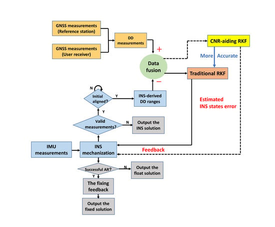
This section describes the TC RTK/INS integration architecture comprehensively. In addition to what we have described above, the INS mechanization and the initial alignment are also important parts of the TC RTK/INS integration. The INS mechanization is a procedure that converts the measurements from the IMU into the position, velocity, and attitude information in the navigation frame [20]. The EKF measurements in the TC RTK/INS integration are calculated based on the INS mechanization results. The states’ errors estimated by the TC RTK/INS integration will be fed back to the INS mechanization to suppress the long-term drift. In our implementation, the INS mechanization operates at the same frequency as the prediction step, whereas the update step operates lower. The initial alignment, which refers to the attitude initialization, aims to obtain the rotation matrix between the body frame and the navigation frame [78]. The TC RTK/INS integration should operate when the initial alignment has been completed. Readers can refer to the documents of PSINS for more details on the INS mechanization and the initial alignment. Notably, when it comes to the outputs, there are three cases. The INS mechanization results will be directly output when there are no valid GNSS measurements. Otherwise, the states’ errors will be estimated by EKF and fed back to the INS mechanization, which generates the float solution. The corresponding fixed INS solution will be output if the ambiguity can be correctly resolved. Table 3 shows these three cases.
Figure 2 illustrates the overview of the TC RTK/INS integration architecture.
2.6. Modified RKF
This section introduces our proposed algorithm that assists RKF. We use the Modified RKF (MRKF) to denote our algorithm to distinguish the traditional IGG-based RKF. The measurements, along with much noise or multipath error, usually provide low CNR. As the multipath effect generally depends on the environment around the receiver, the fault caused by the multipath effect can persist for some epochs. Excessive robustness can happen when RKF incorrectly excludes the measurements that should be retained. We use CNR to decide whether the detected potential outliers can be maintained for a while or not. Specifically, we set two thresholds, and , to classify measurements with different CNR. If a detected outlier’s CNR is smaller than , we discard the measurements immediately as RKF does. If a detected outlier’s CNR is between and , we maintain the measurements for a epoch. The corresponding measurement will be discarded if it is identified as an outlier at the next epoch. If a detected outlier’s CNR exceeds , we maintain the measurements for two epochs. Notably, the corresponding components in will be inflated during the maintaining epochs to downweight the measurements. can be set in a range from 35 decibels-Hz (dBHz) to 40 dBHz, whereas can be set as 45 dBHz. and are set based on our experience. Ref. [79] points out that the dynamic condition and signal strength can determine the true tracking performance. This literature analyzes the relationship between the tracking threshold and the dominant error sources. This literature has carried out many simulations with ideal conditions and concluded that if a measurement’s CNR is lower than 32dBHz, the Phase-Locked Loop (PLL) error will exceed the 1-sigma tracking threshold, degrading the tracking performance. We set to be bigger than 32 dBHz for two reasons. On the one hand, the simulation condition in [79] is ideal. On the other hand, we want to minimize the probability and impact of the wrong retention. When it comes to , a measurement with 45 dBHz CNR can be considered a strong signal of good quality. As decides whether a potential outlier can be maintained for two epochs, we set it as a high value to reduce the wrong retention. Notably, maintaining a measurement for one or two epochs can also be considered thresholds for our algorithm. The epoch here means the time interval between two update steps in the TC RTK/INS integration. We choose a short time for maintenance because the wrong maintenance for a long time can degrade the positioning performance significantly.
Considering that some high-CNR signals can also be superimposed with gross errors, we add some constraints to decide when CNR assistance should be used. If all the DD pseudo-range measurements are identified as outliers, we think the effects of gross errors are significant, and the quality of the signals is poor. In this case, we will not use the CNR-based classification to assist RKF. The DD measurements are calculated separately for the different constellations in our implementation. If all the DD pseudo-range measurements in one constellation are identified as outliers, while no DD pseudo-range measurements in the other constellation are identified as outliers, we believe that one of the constellations provides a very poor quality signal. In this case, we will not use the CNR-based classification to assist RKF. We use these constraints to reduce the probability of incorrectly retaining true outliers. The CNR-based classification and the constraints form MRKF. Figure 3 shows the MRKF architecture.
3. Description of the Datasets
We always need an accurate and reliable reference trajectory to verify our algorithms. The TC RTK/INS researchers generally adopt a navigation product containing a multifrequency receiver and a tactical-grade IMU to collect reliable measurements. After that, some commercial post-processing software like NovAtel’s Waypoint Inertial Explorer [80] is used to provide a reference trajectory to evaluate the improvement of the novel algorithm [36,39,57]. Unfortunately, our laboratory currently lacks the appropriate specialist equipment and commercial software. As a result, we turn to a public dataset provided by Dr. Hsu, Li-Ta, and his team from Hong Kong Polytechnique University [81]. Dr. Li-Ta and his colleagues collect measurements of multi-sensors in Tokyo. They use the Trimble NetR9 to collect the GNSS measurements at 10 Hz and the Tamagawa-seiki TAG264 to collect the IMU measurements at 50 Hz. The ground truth is provided by an Applanix POS LV620 GNSS/INS product. Dr. Li-Ta pointed out that the datasets are collected in harsh urban canyons, which makes the GNSS datasets challenging to process. Furthermore, the team has not provided extrinsic parameters between sensors, which hinders us from obtaining an accurate value of the lever-arm offset. In the relevant experiments in this article, we set the lever-arm offset parameters as zero. This approach is expedient, which can degrade the performance of the high-accuracy positioning. The dataset contains two subsets collected in Shinjuku and Odaiba, respectively. We evaluate our algorithm on both subsets. Figure 4 illustrates the reference trajectories:
4. Results
4.1. The Solution Visualization
In our implementation, the positioning results can be visualized in real time as the program runs. Users can monitor the program’s operation with the solution visualization. Our implementation is based on C++, which does not have the rich visualizing tools of Matlab and Python. Considering the convenience and versatility, we import Matplotlib-cpp, a plotting library wrapping Python visualization tools, into our codes to provide real-time result visualization [82]. Matplotlib-cpp is based on Matplotlib, a comprehensive library for visualizations in Python [83]. Notably, the solution visualization can slow down the speed of the program in processing data. Users can control whether the solution visualization is turned on or off by changing the corresponding parameters in the configuration file. Furthermore, users can also control the program to store solution results, including the position, velocity, and attitude, in a text file for post-processing visualization. Figure 5 illustrates the real-time solution visualization:
4.2. The Performance of the TC RTK/INS Integration without the Outlier Resistance
This section introduces the performance of the TC RTK/INS integration without the outlier resistance. Firstly, we present the availability of GNSS measurements. We compare the DD measurements with the INS-based DD ranges to calculate the residuals in our implementation. The corresponding DD measurement will be discarded if the residuals exceed the empirical threshold. Both RTKLIB and GINAV adopt the same strategy to preprocess the measurements. Figure 6 illustrates the number of preprocessed DD measurements, which equals the dimension of the measurement vector of EKF. As a time-dependent plot over 1000 epochs does not reveal much, we use a histogram to visualize the statistical data. Figure 6 is a histogram that shows the distribution of the occurrence of the measurement number over two datasets. The X-axis in Figure 6 reflects the number of measurements, whereas the Y-axis reflects the number of epochs when the same number of measurements is valid. Figure 6 shows that the number of valid DD measurements in both datasets can be small or even zero. In such cases, RTK can occasionally fail to provide positioning results, which means a GNSS outage can happen. The TC RTK/INS integration can help bridge the outage.
The INS drift can be suppressed in TC integration as long as the number of measurements is not zero. Otherwise, the INS solution can be output as the positioning results. As a result, the TC RTK/INS integration can provide more continuous positioning results when compared to RTK. Furthermore, as we mentioned in the Introduction part, the fixed rate and the positioning accuracy can benefit from the TC integration. However, the outlying measurements can degrade the performance of the TC integration. The datasets are collected in harsh urban areas, which means gross errors frequently occur in GNSS measurements. Figure 7 and Figure 8 show the performance comparison between RTK and the integration without the outlier resistance. Figure 7a,b show the epochs when valid positioning results are provided. In Figure 7a,b, a cycle with a specific color means the specific algorithm can provide a valid positioning result at the corresponding epoch. The local results in the red rectangles are highlighted in the subfigures. In the subfigures, the circles associated with RTK are sparser compared to those associated with the TC RTK/INS integration. Figure 7c,d illustrate the number of epochs in which each algorithm can provide valid positioning results and the number of epochs in which each algorithm cannot provide valid positioning results. Accordingly, Figure 7 demonstrates that the TC RTK/INS integration can provide valid positioning results at every epoch whereas RTK fails to output positioning results from time to time, which means the integration’s positioning continuity is improved. Figure 8 shows the positioning error in meters. In Figure 8, the “TC/EKF” legend denotes the results provided by the TC RTK/INS integration without IGG-based outlier resistance. Figure 8a,b show that the positioning results given by the TC RTK/INS integration are smoother than that given by RTK. There are some large jumps in RTK results, which means gross errors contaminate the measurements and lead to big positioning errors. The introduction of INS reduces the magnitude of the unnormal jumps, which means the integration suppresses the influence of outlying measurements. The integration benefits from the high short-term accuracy of INS, which mitigates the effects of some sudden gross errors. However, the positioning accuracy of the TC RTK/INS integration is not satisfying. At many epochs, the positioning errors provided by the integration are larger than those given by RTK.
In Figure 8a,b, the dots representing the positioning results are too dense, which causes some inconvenience to the visualization. We divide the positioning results into several groups by epochs. Except for the last one, each group contains the positioning results of 100 epochs. Then, we calculate the Root-Mean-Square Error (RMSE) for positioning results in each group. Figure 8c,d show the RMSE results. In Figure 8c, Group 6 corresponds to the positioning results for the 501st epoch to the 600th epoch in Figure 8a. Figure 8a shows, during this period, that some large errors exist in RTK results, especially the results corresponding to the 524th epoch. In contrast, the TC RTK/INS integration provides more accurate positioning results for the 501st epoch to the 600th epoch. Accordingly, the TC RTK/INS integration provides smaller RMSE for results in Group 6. Group 9 is related to the positioning results for the 801st epoch to the 900th epoch in Figure 8a. Figure 8a shows, during this period, that the positioning errors provided by the integration are generally larger than those given by RTK, especially at the 873th epoch. As a result, the TC RTK/INS integration provides a larger RMSE for results in Group 9. We can observe the same phenomenon comparing Figure 8b,d. Figure 8 demonstrates the importance of outlier detection and exclusion. The outlying measurements result in biased estimation and inaccurate INS states correction, which will be accumulated along with the INS mechanization. RKF can help improve the performance of the TC RTK/INS integration. A more specific quantitative analysis will be presented in the next section.
4.3. The Performance of the TC RTK/INS Integration with the Outlier Resistance
Our implementation uses the IGG-III model to inflate the noise covariance matrix components, which can suppress the influence of the outlying measurements. As mentioned in Section 2.3.3, the outlying measurements will be discarded if the corresponding inflation factor is too large. This section introduces the performance of the TC RTK/INS integration with the IGG-III model. Firstly, we present the effects of the IGG-III model on the measurements involved in the TC RTK/INS integration. We use Figure 9 to show in which epochs the outlier exclusion happens and how many measurements are excluded. We subtract the number of measurements after the IGG-based outlier exclusion from that before the outlier exclusion and plot the results in Figure 9. A zero-value subtraction result at an epoch means no outlier exclusion happens at the epoch. In contrast, the outlier exclusion happens, and the value equals the number of the excluded measurements. Notably, the difference results will not fall below zero, as the number of measurements after the outlier exclusion cannot exceed that before the outlier exclusion. Figure 9 illustrates the number difference between valid DD measurements before and after the outlier exclusion. Figure 9 shows that some measurements are regarded as significant outliers and excluded at some epochs, which demonstrates that the IGG-III model plays a role in discarding some potential outlying measurements.
The integration based on the IGG-III model can provide more accurate positioning results when compared to the integration without the outlier resistance. Notably, the introduction of the IGG-III model will not degrade the positioning continuity, which means the integration based on the IGG-III model can provide positioning results during the RTK outage like the integration without the outlier resistance. So, we will not use a figure like Figure 7 to illustrate the positioning continuity of the IGG-based integration. Figure 10 shows the positioning performance comparison between the integration with and without the outlier resistance. Notably, we use RKF to denote the TC RTK/INS integration with the IGG-based outlier resistance. Figure 10 shows the positioning errors in meters. As Figure 10 can provide a qualitative description, we calculate the positioning deviations for the two datasets to quantitatively analyze the positioning performances. Every epoch, we calculate the difference between the positioning result given by different algorithms and the corresponding one given by the reference. Then, we sum up these differences to calculate the RMSE for a dataset. Table 4 and Table 5 show the statistics. For each dataset, we count the total number of epochs between the completion of the initial alignment and termination. Then, we count the number of epochs for which the algorithm can provide positioning results. The ratio of the latter to the former demonstrates the continuity of the algorithm. Table 4 and Table 5 show the TC RTK/INS integration can bridge the RTK outage. Furthermore, the fixed rate benefits from the introduction of INS obviously, whereas the adoption of the IGG-III model brings a slight increase. On the whole, the positioning accuracy of the integration without the outlier resistance is not significantly better than that of RTK or it is even worse. In contrast, the IGG-III model improves the positioning accuracy significantly. Figure 10 and the tables show that the positioning errors given by the IGG-based integration are smaller than those given by the integration without the outlier resistance in general. Comparing Figure 9 and Figure 10, we can see that the epochs with significantly improved positioning accuracy correspond to those in which some potential outlying measurements are discarded, which proves the validity of the IGG-based integration. However, Figure 10 shows that the positioning errors provided by the IGG-based integration can be larger than those given by the integration without the outlier resistance at some epochs. This phenomenon is particularly evident in the Shinjuku dataset, which means that excessive robustness happens. Because the dots denoting positioning results in Figure 10 are too dense, we use two box plots to visualize the distribution of the positioning error for two datasets, as shown in Figure 11. A box plot can visualize the distribution of numerical data and skewness by showing the five-number summary of a set of data, including the lower adjacent, first quartile, median, third quartile, and upper adjacent values [84]. We divide the error results into ten groups by epochs and use a box with two whiskers to show the distribution of errors for each group. In Figure 11a, each group contains 120 results. The boxes of Group 3, Group 4, Group 5, and Group 8 clearly show the error results given by the integration with the outlier resistance have a smaller median, third quartile, and upper adjacent values when compared to those given by the integration without the outlier resistance, which means RKF is superior to EKF for these groups. Let us turn to the results at epochs corresponding to these groups in Figure 10a. We can find that the positioning errors provided by RKF are generally smaller than those provided by EKF. Figure 10a and Figure 11a show that RKF either outperforms or performs comparably to EKF for all the groups. In Figure 11b, each group contains 200 results. The boxes of Group 4 and Group 5 also show the benefits of the IGG-based outlier resistance. The boxes of Group 8 and Group 9 are related to the positioning error results from the 1400th epoch to the 1800th epoch in Figure 10b. Figure 10b shows that excessive robustness happens during the period from time to time. The boxes of Group 8 and Group 9 also show that RKF degrades during this period. The box of Group 9 shows the error results given by RKF have larger third quartile values, and RKF provides a more diffuse error distribution. Our proposed novel algorithm can assist RKF in improving positioning accuracy.
4.4. The Performance of the TC RTK/INS Integration with the Improved Outlier Resistance
4.4.1. Further Analysis of the Shinjuku Dataset
As excessive robustness is more evident when we process the Shinjuku dataset, we further analyze the positioning results of the Shinjuku dataset. The measurements, along with a lot of noise or multipath error, usually provide low CNR. As the multipath effect generally depends on the environment around the receiver, the fault caused by the multipath effect can persist for some epochs. As mentioned in Section 2.3.3, we only inflate the range-related components in . Figure 12 illustrates the excluded pseudo-range measurements and the corresponding CNR. If the test statistic exceeds the second threshold of the IGG-III model, which means a significant gross error happens, IGG-III-based RKF will exclude the corresponding measurement. Notably, the exclusion only happens at the current epoch. When it comes to the next epoch, the test statistic should be calculated again to decide whether the gross error still contaminates the corresponding measurement. In Figure 12, the symbols with different colors and shapes represent different satellites. The specific symbol at an epoch means the corresponding satellite is excluded at this epoch. The Y-axis value corresponding to this symbol indicates the CNR of that satellite for that epoch. A line in a specific color at an epoch means the corresponding satellite contributes to the TC RTK/INS integration.
Figure 12 shows the CNR of the excluded pseudo-range measurements fluctuates over a wide range. Some pseudo-range measurements with high CNR are directly excluded as outliers. Excessive robustness can happen when RKF incorrectly excludes the measurements that should be retained. The CNR can help RKF detect the fault more reliably.
Figure 13 shows the positioning error from the 1720th epoch to the 1770th epoch. Excessive robustness happens as the positioning error given by the IGG-based integration can be larger than that given by the integration without the outlier resistance. The turning points are the 1731st epoch and the 1732nd epoch, which are marked with two rectangles. Figure 14 illustrates the excluded pseudo-range measurements and the corresponding CNR from the 1720th epoch to the 1755th epoch. We use two red rectangles to highlight the excluded measurements at the 1731st epoch and the 1732nd epoch corresponding to the turning points in Figure 13. If a symbol with a specific shape appears in the rectangle, the corresponding measurements will be discarded and not contribute to positioning at a certain epoch. In contrast, a line in a certain color in the rectangular means the corresponding measurement is retained for positioning. Figure 14a shows that conventional RKF excludes some potential outlying GPS pseudo-range measurements at both the 1731st epoch and the 1732nd epoch. Meanwhile, no BDS pseudo-range measurements are treated as outliers. The pseudo range of the 24th GPS satellites is detected to be faulty for only two epochs, whereas the CNR is around 42 dBHz, which means the signal quality is quite good. Notably, RKF excludes all the pseudo-range measurements at the 1731st epoch and only excludes the pseudo range of the 24th GPS satellites at the 1732nd epoch. We manually control the operation of the outlier exclusion following our proposed algorithm at the 1731st epoch and the 1732nd epoch to see the influence. Specifically, we exclude all the pseudo-range measurements at the 1731st epoch as traditional RKF does and retain the pseudo range of the 24th GPS satellites at the 1732nd epoch. Furthermore, we inflate the corresponding components in . The results are presented in Figure 15. Figure 15 shows that the manual control based on our proposed algorithm reduces the positioning error when compared to conventional RKF. This fact demonstrates that it is feasible and valid to retain some detected outliers based on the CNR to resist excessive robustness.
4.4.2. The Performance of MRKF
This section introduces the performance of the TC RTK/INS integration with improved outlier resistance. We use MRKF to denote our proposed CNR-assisting algorithm to distinguish it from the traditional IGG-based RKF. As mentioned in Section 2.6, MRKF can be divided into the CNR-based classification and the constraints. The CNR-based classification aims to suppress excessive robustness, whereas the constraints reduce the probability of incorrectly retaining true outliers. Figure 16 illustrates the performance of MRKF with and without the constraints. Figure 16a,b both show that the positioning accuracy is improved around the 1500th epoch and the 1730th epoch. The CNR-based classification maintains some measurements that are incorrectly identified as outliers, which reduces the effects of excessive robustness and provides more accurate positioning results. In Figure 16a, there are two time periods when the positioning errors given by MRKF without the constraints are larger than those given by RKF, which means some outliers are retained incorrectly because of high CNR. Figure 16b shows that the constraints eliminate improper maintenance.
As the dots denoting positioning results in Figure 16 are too dense, we use a box plot to visualize the distribution of the positioning error to compare TC/EKF, TC/RKF, and TC/MRKF, as shown in Figure 17. In Figure 17, each group contains 200 results. The boxes of Group 8 and Group 9 are related to the positioning error results from the 1400th epoch to the 1800th epoch in Figure 16b. The boxes of Group 8 and Group 9 show that MRKF significantly reduces the first quartile, median, and third quartile values compared to RKF, which shows MRKF generally provides more accurate positioning results when compared to RKF during the corresponding period. Overall, RKF either outperforms or performs comparably to RKF for all the groups.
Figure 18 shows the positioning error in three dimensions. Notably, Figure 18 shows the positioning error and not the absolute value of the error as in Figure 16. Figure 16 and Figure 18 qualitatively show the combination of the CNR-based classification and the constraints can improve the positioning accuracy reliably. We calculate the RMSE of RKF and MRKF in three dimensions and total. The statistics are presented in Table 6. Table 6 and Figure 18 also contain the results given by RTK and the TC RTK/INS integration without the outlier resistance. Furthermore, Table 6 shows that MRKF makes a small contribution to AR.
Figure 10 shows that evident excessive robustness happens in the Shinjuku dataset, whereas no apparent excessive robustness happens in the Odaiba dataset. We test the performance of MRKF on the Odaiba dataset to see whether our proposed algorithm will degrade when processing datasets without evident excessive robustness. The results are based on the same CNR thresholds as those used when processing the Shinjuku dataset. Figure 19 illustrates the positioning error in three dimensions. Figure 20a compares the total positioning error given by three algorithms at each epoch. Figure 20b is a box plot that visualizes the distribution of the positioning error for each group. In Figure 20b, each group contains 120 positioning results. Figure 20a shows the positioning error of RKF and MRKF is essentially the same at each epoch, whereas Figure 20b shows that the error distribution for each group is essentially the same. Figure 20 illustrates that MRKF performs comparably to RKF for the Odaiba dataset. Table 7 shows the quantitative analysis for the Odaiba dataset. Figure 19 and Figure 20 and Table 7 show that the positioning accuracy is essentially the same for RKF and MRKF. These facts say that MRKF will not reduce positioning accuracy when processing datasets where no evident excessive robustness happens. Tests on the Shinjuku and Odaiba datasets verify our proposed algorithm’s validity and feasibility in using CNR to assist traditional RKF.
5. Discussion
This section provides a summary and analysis of the results. Firstly, we present the visualization window of our open-source TC RTK/INS implementation. Next, we compare the positioning performances of RTK and the TC RTK/INS integration. The introduction of INS improves the positioning continuity and the fixed rate. RTK can provide positioning results at no more than 90 percent of the epochs for both datasets, whereas the integration can provide positioning results at every epoch. The fixed rate increases by for the Odaiba dataset and for the Shinjuku dataset. However, the integration does not significantly improve positioning accuracy because of the outliers. Then, we compare the positioning performance of the TC RTK/INS integration with and without the outlier resistance. IGG-based RKF uses inflation factors to suppress the outliers. If the inflation factor is too large, RKF will discard the corresponding measurements. RKF generates a significant improvement in positioning accuracy on both datasets. The RMSE has been reduced from m to m on the Odaiba dataset and from m to m on the Shinjuku dataset. However, obvious excessive robustness happens in the Shinjuku dataset. Taking this into account, we improve the RKF to prevent excessive robustness. We use MRKF to denote our proposed algorithm. MRKF can be divided into two parts: the CNR-based classification and the constraints. The CNR-based classification aims to maintain some measurements that are incorrectly identified as outliers. The constraints reduce the probability of incorrectly retaining true outliers. MRKF improves the positioning accuracy for the Shinjuku dataset. RMSE has been reduced from m to m. When it comes to the Odaiba dataset without obvious excessive robustness, MRKF will not reduce the positioning accuracy. RMSE has been changed from m to m.
6. Conclusions
This study introduces the TC RTK/INS integration implementation in detail. We give some derivations of key issues, including the formulation of the observation matrix and the process to obtain the fixed solution. We open source our implementation to help save the effort and cost of the researchers who are in the same field as us. These codes can be found at https://github.com/Nronaldo, accessed on 2 April 2022. We test the positioning performance of the TC RTK/INS integration on two open-source urban area datasets. The results show that the introduction of INS improves the positioning continuity and the fixed rate. As outlying measurements frequently appear in urban areas, the TC RTK/INS integration without the outlier resistance cannot obviously improve the positioning accuracy. The IGG-based TC RTK/INS integration uses an inflation factor to suppress the effects of the outliers, which significantly improves the positioning accuracy for both datasets. As excessive robustness occasionally happens, we propose a CNR-based algorithm to decide whether a detected outlier should be maintained for a while or not. Our proposed algorithm improves the positioning accuracy for the Shinjuku dataset, which presents evident excessive robustness. When it comes to the Odaiba dataset without obvious excessive robustness, our proposed algorithm will not degrade the positioning accuracy.
There is still a lot of room for improvement in our work. Two datasets can only verify the algorithm feasibility on some occasions. Furthermore, our open-source implementation is only a preliminary architecture. It does not represent the state of the art. The architecture needs more modules, including reliable cycle slip repair, gross error preprocessing, and fixed solution verification. We will design the hardware platform to collect more datasets in urban areas in the future. We will seek to obtain professional devices and commercial software to provide the reference trajectory and improve our proposed algorithm. We will also develop our current implementation and add new functional modules to our open-source architecture.
Author Contributions
Conceptualization, Z.N.; formal analysis, Z.N., F.G., Q.S. and G.L.; software, Z.N.; writing, original draft, Z.N.; writing, review and editing, Z.N. and B.Z. All authors have read and agreed to the published version of the manuscript.
Funding
This research was funded by the National Key Research and Development Project of China, Grant Number 2020YFB0505602-02.
Acknowledgments
The authors thank the team from Hong Kong Polytechnique University for providing the Tokyo datasets that can be found in https://github.com/weisongwen/UrbanNavDataset, accessed on 2 April 2022. The authors thank the authors of RTKLIB, PSINS, and GINAV for selflessly providing open-source codes.
Conflicts of Interest
The authors declare no conflict of interest.
Appendix A. The Derivation of the Observation Matrix
Let us ignore the lever-arm offset for a moment. We assume there are two satellites, and , and the position error is added to the true position as Figure A1 shows:
Figure A1.
The position error and the lever-arm offset.

The position error can only result in a distance error between the satellites and the user receiver because the reference station is accurately localized. Because the position error is small, the LOS vector from the true position to a satellite is the same as that from the nominal position to the satellite. Furthermore, the change in the distance between the satellite and the receiver can be calculated based on the LOS vector and the change of the receiver’s position, as Equation (A1) shows [70]:
Accordingly, the nominal DD distance and the true DD distance can be formulated as Equation (A2) shows:
Because we neglect the lever-arm offset, the INS position is the same as the GNSS antenna. Considering Equations (3) and (4), we can calculate a component of the measurement vector as:
Equation (A3) shows that only the position error and the SD ambiguity in the state vector contribute to the measurement vector when we neglect the lever-arm offset. Considering all the available satellites, we can obtain Equation (A4):
Readers can refer to the documents of PSINS to find the details about the transformation matrix .
The attitude error can generate a position error when the lever-arm offset exists. Figure A1 illustrates the lever-arm offset in the body frame. We use and to denote the lever-arm offset in the body frame and ECEF frame, respectively. As the measurement vector is calculated in the ECEF frame, we should calculate the position of the GNSS antenna based on the INS position and . If there is no error, can be formulated as Equation (A5) shows:
In Equation (A5), the attitude error will not influence as it can be directly calculated using the position. Considering the attitude error , we can calculate the nominal lever-arm offset in ECEF frame , as Equation (A6) shows:
where is the position error in ECEF frame, which is caused by the attitude error and the lever-arm offset. Accordingly, we can formulate in Equation (12), as Equation (A7) shows:
References
- GNSS & Surveying 2017: The Year in Review. Available online: https://www.gpsworld.com/gnss-surveying-2017-the-year-in-review/ (accessed on 31 March 2022).
- The Almanac. Available online: https://www.gpsworld.com/the-almanac/ (accessed on 31 March 2022).
- Varbla, S.; Puust, R.; Ellmann, A. Accuracy assessment of RTK-GNSS equipped UAV conducted as-built surveys for construction site modelling. Survey Rev. 2020, 53, 477–492. [Google Scholar] [CrossRef]
- Rietdorf, A.; Daub, C.; Loef, P. Precise positioning in real-time using navigation satellites and telecommunication. In Proceedings of the 3rd Workshop on Positioning, Navigation and Communication (WPNC’06), Hannover, Germany, 16–19 March 2006; pp. 209–218. [Google Scholar]
- Takasu, T.; Kubo, N.; Yasuda, A. Development, evaluation and application of RTKLIB: A program library for RTK-GPS. In Proceedings of the 2007 GPS/GNSS Symposium, Tokyo, Japan, 20–22 November 2007. [Google Scholar]
- Teunissen, P.; Montenbruck, O. Basic observation equations. In Handbook of Global Navigation Satellite Systems, 1st ed.; Springer: Berlin/Heidelberg, Germany, 2017; ISBN 978-3-319-42926-7. [Google Scholar]
- Lee, I.S.; Ge, L. The performance of RTK-GPS for surveying under challenging environmental conditions. Earth Planets Sp. 2006, 58, 515–522. [Google Scholar] [CrossRef] [Green Version]
- Gao, W.; Gao, C.F.; Pan, S.G.; Wang, D.H.; Wang, S.L. Single-epoch positioning method in network RTK with BDS triple-frequency widelane combinations. Acta Geod. Cartogr. Sin. 2015, 44, 641–648. Available online: http://xb.sinomaps.com/EN/10.11947/j.AGCS.2015.20140308 (accessed on 2 April 2022).
- Deng, C.L.; Tang, W.M.; Liu, J.N.; Shi, C. Reliable single-epoch ambiguity resolution for short baselines using combined GPS/BeiDou system. GPS Solut. 2014, 18, 375–386. [Google Scholar] [CrossRef]
- Gao, W.; Gao, C.F.; Pan, S.G.; Yu, G.R.; Hu, H.Q. Method and assessment of BDS triple-frequency ambiguity resolution for long-baseline network RTK. Adv. Space Res. 2017, 60, 2520–2532. [Google Scholar] [CrossRef]
- Carcanague, S.; Julien, O.; Vigneau, W.; Macabiau, C. Low-cost single-frequency GPS/GLONASS RTK for road users. In Proceedings of the ION 2013 Pacific PNT Meeting, Honolulu, HI, USA, 23–25 April 2013; pp. 168–184. [Google Scholar]
- Li, T.; Zhang, H.P.; Niu, X.J.; Gao, Z.Z. Tightly-coupled integration of multi-GNSS single-Frequency RTK and MEMS-IMU for enhanced positioning performance. Sensors 2017, 17, 2462. [Google Scholar] [CrossRef] [Green Version]
- Montenbruck, O.; Steigenberger, P.; Prange, L.; Deng, Z.; Zhao, Q.; Perosanz, F.; Romero, I.; Noll, C.; Stürze, A.; Weber, G.; et al. The Multi-GNSS Experiment (MGEX) of the International GNSS Service (IGS) – achievements, prospects and challenges. Adv. Space Res. 2017, 59, 1671–1697. [Google Scholar] [CrossRef]
- Odolinski, R.; Teunissen, P.J.G. Single-frequency, dual-GNSS versus dual-frequency, single-GNSS: A low-cost and high-grade receivers GPS-BDS RTK analysis. J. Geod. 2016, 90, 1255–1278. [Google Scholar] [CrossRef]
- Odijk, D.; Teunissen, P. Characterization of between-receiver GPS-Galileo inter-system biases and their effect on mixed ambiguity resolution. GPS Solut. 2013, 17, 521–533. [Google Scholar] [CrossRef]
- Odolinski, R.; Odijk, D.; Teunissen, P. Combined BDS, Galileo, QZSS and GPS single-frequency RTK. GPS Solut. 2015, 19, 151–163. [Google Scholar] [CrossRef]
- Sinko, J.W. RTK performance in highway and racetrack experiments. J. Inst. Navig. 2003, 50, 265–276. [Google Scholar] [CrossRef]
- Yang, C.; Shi, W.; Chen, W. Correlational inference-based adaptive unscented Kalman filter with application in GNSS/IMU-integrated navigation. GPS Solut. 2018, 22, 1–14. [Google Scholar] [CrossRef]
- Kirkko-Jaakkola, M.; Ruotsalainen, L.; Bhuiyan, M.Z.H.; Söderholm, S.; Thombre, S.; Kuusniemi, H. Performance of a MEMS IMU deeply coupled with a GNSS receiver under jamming. 2014 Ubiquitous Positioning Indoor Navigation and Location Based Service (UPINLBS), Corpus Christi, TX, USA, 20–21 November 2014; pp. 64–70. [Google Scholar]
- Angrisano, A. GNSS/INS integration methods. Ph.D. Thesis, The Parthenope University of Naples, Naples, Italy, 2010. [Google Scholar]
- Li, T.; Zhang, H.P.; Gao, Z.Z.; Niu, X.J.; El-sheimy, N. Tight fusion of a monocular camera, MEMS-IMU, and single-frequency multi-GNSS RTK for precise navigation in GNSS-challenged environments. Remote. Sens. 2019, 11, 610. [Google Scholar] [CrossRef] [Green Version]
- Schütz, A.; Sánchez-Morales, D.E.; Pany, T. Precise positioning through a loosely-coupled sensor fusion of GNSS-RTK, INS and LiDAR for autonomous driving. In Proceedings of the 2020 IEEE/ION Position, Location and Navigation Symposium (PLANS), Portland, OR, USA, 20–23 April 2020; pp. 219–225. [Google Scholar]
- El-Mowafy, A.; Kubo, N. Integrity monitoring for positioning of intelligent transport systems using integrated RTK-GNSS, IMU and vehicle odometer. IET Intell. Transp. Syst. 2018, 12, 901–908. [Google Scholar] [CrossRef] [Green Version]
- Sun, J.R.; Tao, L.; Niu, Z.; Zhu, B.C. An improved adaptive unscented Kalman filter with application in the deeply integrated BDS/INS navigation system. IEEE Access 2020, 8, 95321–95332. [Google Scholar] [CrossRef]
- Wang, J.; Liu, D.; Jiang, W.; Lu, D.B. Evaluation on loosely and tightly coupled GNSS/INS vehicle navigation system. In Proceedings of the 2017 International Conference on Electromagnetics in Advanced Applications (ICEAA), Verona, Italy, 11–15 September 2017; pp. 892–895. [Google Scholar]
- Jwo, D.J.; Yang, C.F.; Chuang, C.H.; Lin, K.C. A novel design for the ultra-tightly coupled GPS/INS navigation system. J. Navig. 2012, 65, 717–747. [Google Scholar] [CrossRef] [Green Version]
- Falco, G.; Pini, M.; Marucco, G. Loose and tight GNSS/INS integrations: Comparison of performance assessed in real urban scenarios. Sensors 2017, 17, 255. [Google Scholar] [CrossRef]
- Weiss, J.D.; Kee, D.S. A direct performance comparison between loosely coupled and tightly coupled GPS/INS integration techniques. In Proceedings of the 51st Annual Meeting of The Institute of Navigation, Colorado Springs, CO, USA, 5–7 June 1995; pp. 537–544. [Google Scholar]
- Sun, J.R.; Niu, Z.; Zhu, B.C. Fault detection and exclusion method for a deeply integrated BDS/INS system. Sensors 2020, 20, 1844. [Google Scholar] [CrossRef] [Green Version]
- Alban, S.; Akos, D.M.; Rock, S.M. Performance analysis and architectures for INS-aided GPS tracking loops. In Proceedings of the 2003 National Technical Meeting of The Institute of Navigation (NTM), Anaheim, CA, USA, 22–24 January 2003; pp. 611–622. [Google Scholar]
- Imparato, D.; Floch, J.J. INS/GNSS fusion. In Proceedings of the Airbus Defence and Space, Ottobrunn, Germany, 11 February 2019; Available online: https://ec.europa.eu/research/participants/documents/downloadPublic?documentIds=080166e5c206c883&appId=PPGMS (accessed on 2 April 2022).
- Dai, Z. MATLAB software for GPS cycle-slip processing. GPS Solut. 2012, 16, 267–272. [Google Scholar] [CrossRef] [Green Version]
- Takasu, T.; Yasuda, A. Cycle slip detection and fixing by MEMS-IMU/GPS integration for mobile environment RTK-GPS. In Proceedings of the 21st International Technical Meeting of the Satellite Division of The Institute of Navigation (ION GNSS 2008), Savannah, GA, USA, 16–19 September 2008; pp. 64–71. [Google Scholar]
- Kim, Y.; Song, J.; Ho, Y.; Kee, C.; Park, B. Optimal selection of an inertial sensor for cycle slip detection considering single-frequency RTK/INS integrated navigation. Trans. Japan Soc. Aero. Space Sci. 2016, 59, 205–217. [Google Scholar] [CrossRef] [Green Version]
- Chen, K.; Chang, G.B.; Chen, C.; Zhu, T. An improved TDCP-GNSS/INS integration scheme considering small cycle slip for low-cost land vehicular applications. Meas. Sci. Technol. 2021, 32, 055006. [Google Scholar] [CrossRef]
- Scherzinger, B.M. Robust positioning with single frequency inertially aided RTK. In Proceedings of the 2002 National Technical Meeting of The Institute of Navigation, San Diego, CA, USA, 28–30 January 2002; pp. 911–917. [Google Scholar]
- Done, M.; Filwarny, J.O.; Wieser, M. Inertially-aided RTK based on tightly-coupled integration using low-cost GNSS receivers. In Proceedings of the 2017 European Navigation Conference (ENC), Lausanne, Switzerland, 9–12 May 2002; pp. 186–197. [Google Scholar]
- Li, W.; Li, W.Y.; Cui, X.W.; Zhao, S.H.; Lu, M.Q. A tightly coupled RTK/INS algorithm with ambiguity resolution in the position domain for ground vehicles in harsh urban environments. Sensors 2018, 18, 2160. [Google Scholar] [CrossRef] [PubMed] [Green Version]
- Li, T.; Zhang, H.P.; Gao, Z.Z.; Chen, Q.J.; Niu, X.J. High-accuracy positioning in urban environments using single-frequency multi-GNSS RTK/MEMS IMU integration. Remote. Sens. 2018, 10, 205. [Google Scholar] [CrossRef] [Green Version]
- Li, Q.F.; Ai, L.; Xiao, J.P.; Hsu, L.T.; Kamijo, S.; Gu, Y.L. Tightly coupled RTK/MIMU using single frequency BDS/GPS/QZSS receiver for automatic driving vehicle. In Proceedings of the 2018 IEEE/ION Position, Location and Navigation Symposium (PLANS), Monterey, CA, USA, 23–26 April 2018; pp. 185–189. [Google Scholar]
- Zhu, S.; Li, S.H.; Liu, Y.; Fu, Q.W.; Kamijo, S.; Gu, Y.L. Low-cost MEMS-IMU/RTK tightly coupled vehicle navigation system with robust lane-level position accuracy. In Proceedings of the 2019 26th Saint Petersburg International Conference on Integrated Navigation Systems (ICINS), St. Petersburg, Russia, 27–29 May 2019; pp. 1–4. [Google Scholar]
- Li, T.; Zhang, H.P.; Niu, X.J.; Zhang, Q. Performance analysis of tightly coupled RTK/INS algorithm in case of insufficient number of satellites. Remote. Sens. 2018, 43, 478–484. [Google Scholar] [CrossRef]
- Wang, D.J.; Dong, Y.; Li, Z.Y.; Li, Q.S.; Wu, J. Constrained MEMS-Based GNSS/INS tightly coupled system with robust Kalman filter for accurate land vehicular navigation. IEEE Trans. Ins. Meas. 2020, 69, 5138–5148. [Google Scholar] [CrossRef]
- Dong, Y.; Wang, D.J.; Zhang, L.; Li, Q.S.; Wu, J. Tightly coupled GNSS/INS integration with robust sequential Kalman filter for accurate vehicular navigation. Sensors 2020, 20, 561. [Google Scholar] [CrossRef] [Green Version]
- De Jong, C.D.; Marel, H.V.; Jonkman, N.F. Real-time GPS and GLONASS integrity monitoring and reference station software. Phys. Chem. Earth Part Solid Earth Geod. 2001, 26, 545–549. [Google Scholar] [CrossRef]
- Teunissen, P.J.G. Quality control in integrated navigation systems. In Proceedings of the IEEE Symposium on Position Location and Navigation. A Decade of Excellence in the Navigation Sciences, Las Vegas, NV, USA, 20 March 1990; pp. 158–165. [Google Scholar]
- Gillissen, I.; Elema, I.A. Test results of DIA: A real-time adaptive integrity monitoring procedure, used in an integrated naviation system. Int. Hydrogr. Rev. 1996, 73, 75–100. [Google Scholar]
- Hewitson, S.; Wang, J.L. Extended receiver autonomous integrity monitoring (eRAIM) for GNSS/INS integration. J. Surveying Eng. 2010, 136, 13–22. [Google Scholar] [CrossRef] [Green Version]
- Sage, A.P.; Husa, G.W. Adaptive filtering with unknown prior statistics. In Proceedings of the 10th Joint Automatic Control Conference, Boulder, CO, USA, 5–7 August 1969; pp. 760–769. [Google Scholar]
- Xu, S.Q.; Zhou, H.Y.; Wang, J.Q.; He, Z.M.; Wang, D.Y. SINS/CNS/GNSS integrated navigation based on an improved federated Sage–Husa adaptive filter. Sensors 2019, 19, 3812. [Google Scholar] [CrossRef] [Green Version]
- Koch, K.R.; Yang, Y. Robust Kalman filter for rank deficient observation models. J. Geod. 1998, 72, 436–441. [Google Scholar] [CrossRef]
- Jiang, C.; Zhang, S.B.; Li, H.; Li, Z. Performance evaluation of the flters with adaptive factor and fading factor for GNSS/INS integrated systems. GPS Solut. 2021, 25, 130–141. [Google Scholar] [CrossRef]
- Yang, Y.X.; Cui, X.Q. Adaptively robust filter with multi adaptive factors. Survey Rev. 2008, 40, 260–270. [Google Scholar] [CrossRef]
- Crespillo, O.G.; Medina, D.; Skaloud, J.; Meurer, M. Tightly coupled GNSS/INS integration based on robust M-estimators. 2018 IEEE/ION Position, Location and Navigation Symposium (PLANS), Monterey, CA, USA, 23–26 April 2018; pp. 1554–1561. [Google Scholar]
- Yang, Y.X.; Ren, X.; Xu, Y. Main progress of adaptively robust filter with applications in navigation. J. Navig. Pos. 2013, 1, 9–15. [Google Scholar] [CrossRef]
- Gao, B.B.; Hu, G.G.; Zhong, Y.M.; Zhu, X.H. Cubature Kalman filter with both adaptability and robustness for tightly-coupled GNSS/INS integration. IEEE Sensors J. 2021, 21, 14997–15011. [Google Scholar] [CrossRef]
- Yang, Z.H.; Li, Z.K.; Liu, Z.; Wang, C.C.; Sun, Y.W.; Shao, K.F. Improved robust and adaptive filter based on non-holonomic constraints for RTK/INS integrated navigation. Meas. Sci. Technol. 2021, 32, 105110. [Google Scholar] [CrossRef]
- Zhang, Q.Q.; Zhao, L.D.; Zhao, L. A two-step robust adaptive filtering algorithm for GNSS kinematic precise point positioning. Chinese J. Aero. 2021, 34, 210–219. [Google Scholar] [CrossRef]
- Zhang, Q.Q.; Zhao, L.; Zhou, J.H. Two-step robust adaptive filtering with application to PPP/INS integrated navigation. Navig. Pos. Timing 2020, 7. [Google Scholar] [CrossRef]
- Yue, Z.; Lian, B.W.; Tong, K.X.; Chen, S.H. Novel strong tracking square-root cubature Kalman filter for GNSS/INS integrated navigation system. IET Radar Sonar Navig. 2019, 13, 976–982. [Google Scholar] [CrossRef]
- Li, Z.K.; Gao, J.X.; Wang, J.; Yao, Y.F. PPP/INS tightly coupled navigation using adaptive federated filter. GPS Solut. 2017, 21, 137–148. [Google Scholar] [CrossRef]
- Takasu, T.; Yasuda, A. Development of the low-cost RTK-GPS receiver with an open source program package RTKLIB. In Proceedings of the International Symposium on GPS/GNSS, Jeju, Korea, 4–6 November 2009. [Google Scholar]
- Chen, C.; Chang, G.B. PPPLib: An open-source software for precise point positioning using GPS, BeiDou, Galileo, GLONASS, and QZSS with multi-frequency observations. GPS Solut. 2020, 25, 18. [Google Scholar] [CrossRef]
- Yan, G.M. PSINS. Available online: http://www.psins.org.cn/kydm (accessed on 31 March 2022).
- Chen, K.; Chang, G.B.; Chen, C. GINav: A MATLAB-based software for the data processing and analysis of a GNSS/INS integrated navigation system. GPS Solut. 2021, 25, 108. [Google Scholar] [CrossRef]
- i2Nav-WHU. OB-GINS. Available online: https://github.com/i2Nav-WHU/OB_GINS (accessed on 31 March 2022).
- Niu, Z.; Guo, F.G.; Shuai, Q.Q.; Li, G.C.; Zhu, B.C. The integration of GPS/BDS real-time kinematic positioning and visual–inertial odometry based on smartphones. ISPRS Int. J. Geo-Inf. 2021, 10, 699. [Google Scholar] [CrossRef]
- Terejanu, G.A. Extended Kalman filter tutorial. University at Buffalo. 2008. Available online: https://homes.cs.washington.edu/~todorov/courses/cseP590/readings/tutorialEKF.pdf (accessed on 2 April 2022).
- Teunissen, P.J.G. The least-squares ambiguity decorrelation adjustment: A method for fast GPS integer ambiguity estimation. J. Geod. 1995, 70, 65–82. [Google Scholar] [CrossRef]
- Xie, G. Precise positioning systems. In Principles of GPS and Receiver Design, 1st ed.; Publishing House of Electronics Industry: Beijing, China, 2017; Volume 7, pp. 166–171. ISBN 978-7-121-09077-6. [Google Scholar]
- Chen, K. GINAV Manual. Available online: https://github.com/kaichen686/GINav (accessed on 31 March 2022).
- IMU Noise Model. Available online: https://github.com/ethz-asl/kalibr/wiki/IMU-Noise-Model (accessed on 31 March 2022).
- El-Sheimy, N.; Hou, H.Y.; Niu, X.J. Analysis and modeling of inertial sensors using Allan Variance. IEEE Trans. Ins. Meas. 2008, 57, 140–149. [Google Scholar] [CrossRef]
- Takasu, T. RTKLIB ver. 2.4.2 Manual. Available online: http://www.rtklib.com/prog/manual_2.4.2.pdf (accessed on 31 March 2022).
- Li, T. Research on the tightly coupled singlefrequency multi-GNSS/INS/Vision integration for precise position and orientation estimation. Ph.D. Thesis, Wuhan University, Wuhan, China, 2019. [Google Scholar]
- Zhang, Q.Q.; Zhao, L.; Zhou, J.H. A novel weighting approach for variance component estimation in GPS/BDS PPP. IEEE Sensors J. 2019, 19, 3763–3771. [Google Scholar] [CrossRef]
- Yang, Y.X.; Song, L.; Xu, T. Robust estimator for correlated observations based on bifactor equivalent weights. J. Geod. 2002, 76, 353–358. [Google Scholar] [CrossRef]
- Han, H.Z.; Wang, J.; Du, M.Y. A fast SINS initial alignment method based on RTS forward and backward resolution. J. Sensors 2017, 2017. [Google Scholar] [CrossRef]
- Kaplan, E.D.; Hegarty, C.J. Measurement errors and tracking thresholds. In Understanding GPS/GNSS Principles and Applications, 3rd ed.; Artech House: Norwood, MA, USA, 2017; ISBN 978-1-63081-058-0. [Google Scholar]
- Kennedy, S.; Hamilton, J.; Martell, H. Architecture and system performance of SPAN-NovAtel’s GPS/INS solution. In Proceedings of the 2006 IEEE/ION Position, Location, and Navigation Symposium, Coronado, CA, USA, 25–27 April 2006. [Google Scholar]
- Li-Ta, H.; Kubo, N.; Wen, W.S.; Chen, W.; Liu, Z.Z.; Suzuki, T.; Meguro, J. UrbanNav: An open-sourced multisensory dataset for benchmarking positioning algorithms designed for urban areas. In Proceedings of the 34th International Technical Meeting of the Satellite Division of The Institute of Navigation (ION GNSS+ 2021), St. Louis, MO, USA, 22–25 September 2021. [Google Scholar]
- Matplotlib-cpp. Available online: https://github.com/lava/matplotlib-cpp (accessed on 31 March 2022).
- Hunter, J.D. Matplotlib: A 2D Graphics Environment. Comput. Sci. Eng. 2007, 9, 90–95. [Google Scholar] [CrossRef]
- Wang, L.; Li, Z.S.; Wang, N.B.; Wang, Z.Y. Real-time GNSS precise point positioning for low-cost smart devices. GPS Solut. 2021, 25, 69. [Google Scholar] [CrossRef]
Figure 1.
SD measurements and DD measurements. (a) Two receivers track the signals of two satellites. (b) Steps to calculate SD measurements and DD measurements.
Figure 1.
SD measurements and DD measurements. (a) Two receivers track the signals of two satellites. (b) Steps to calculate SD measurements and DD measurements.

Figure 2.
The overview of the TC RTK/INS integration architecture.

Figure 3.
The MRKF architecture.

Figure 4.
The reference trajectories of the datasets.


Figure 5.
The solution visualization.


Figure 6.
The number distribution of preprocessed DD measurements.

Figure 7.
The positioning continuity comparison between RTK and TC RTK/INS.


Figure 8.
The positioning accuracy comparison between RTK and the TC RTK/INS integration.

Figure 9.
The number of the excluded measurements.

Figure 10.
The positioning accuracy comparison between the integration with and without the outlier resistance.
Figure 10.
The positioning accuracy comparison between the integration with and without the outlier resistance.

Figure 11.
The box plots show comparison between the integration with and without the outlier resistance.
Figure 11.
The box plots show comparison between the integration with and without the outlier resistance.

Figure 12.
The excluded pseudo-range measurements and the corresponding CNR.

Figure 13.
The positioning error in local.

Figure 14.
The excluded pseudo-range measurements and the corresponding CNR in local.

Figure 15.
The comparison between the performances with and without the manual control.

Figure 16.
The performances of MRKF with and without the constraints.

Figure 17.
The box plot showing the performance of MRKF.

Figure 18.
The position error in three dimensions (Shinjuku).

Figure 19.
The positioning error in three dimensions (Odaiba).

Figure 20.
The performances of MRKF for the Odaiba dataset.


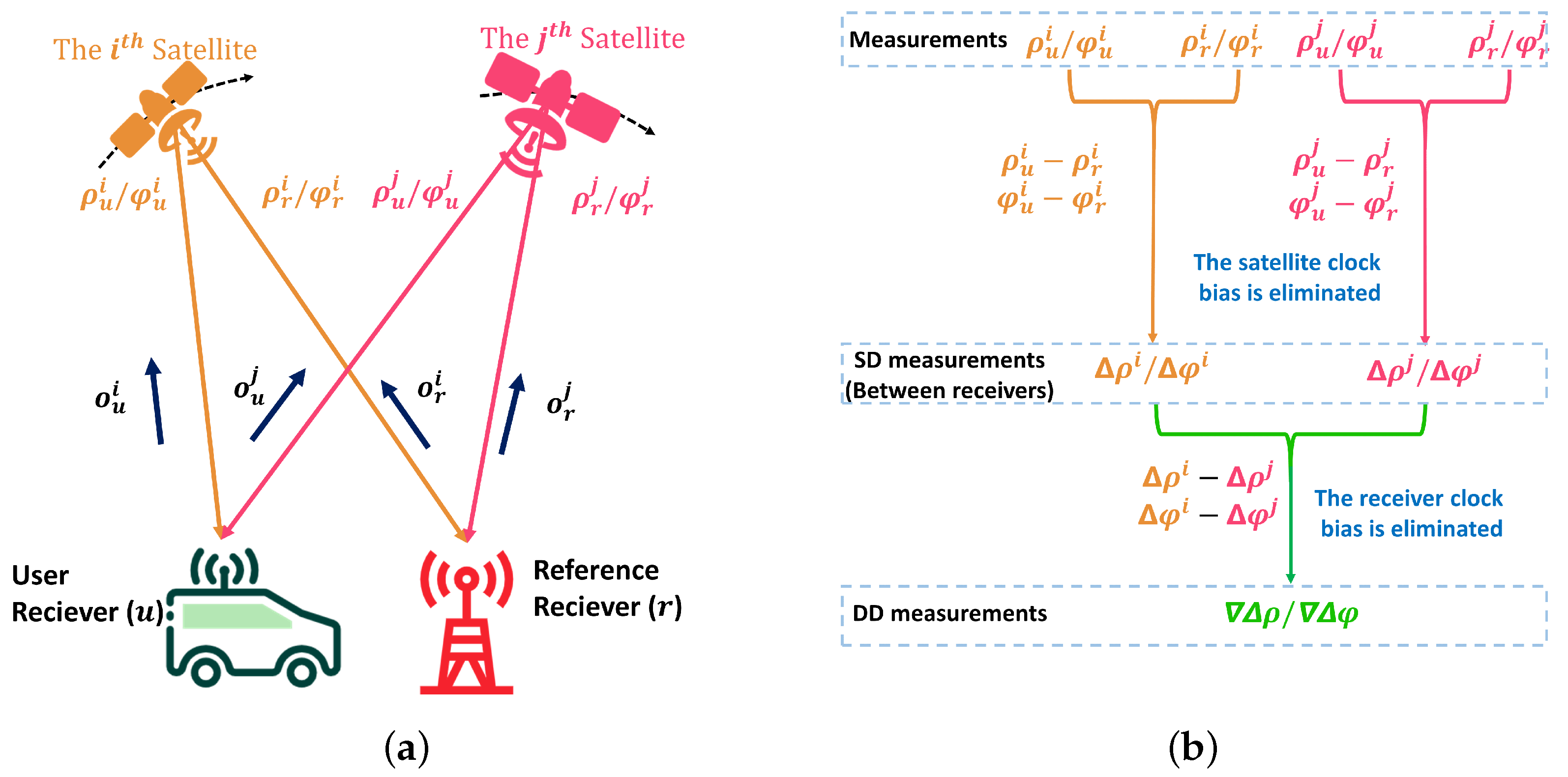
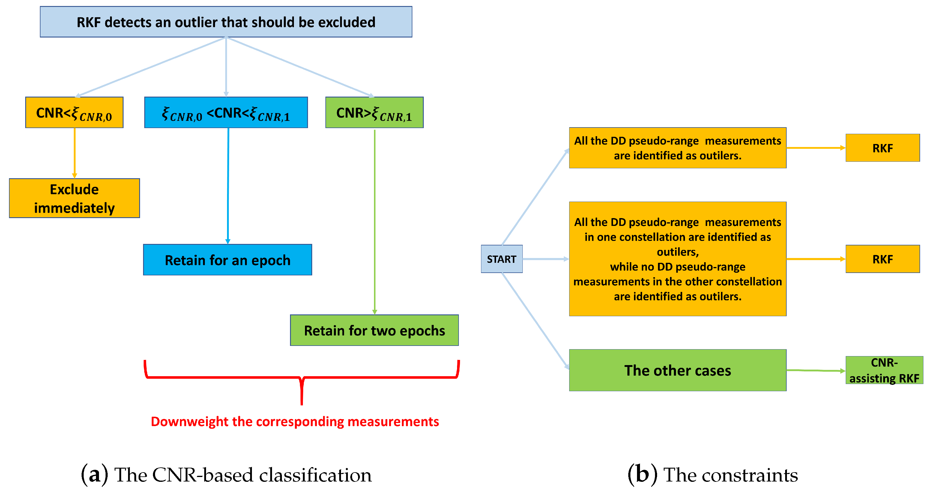
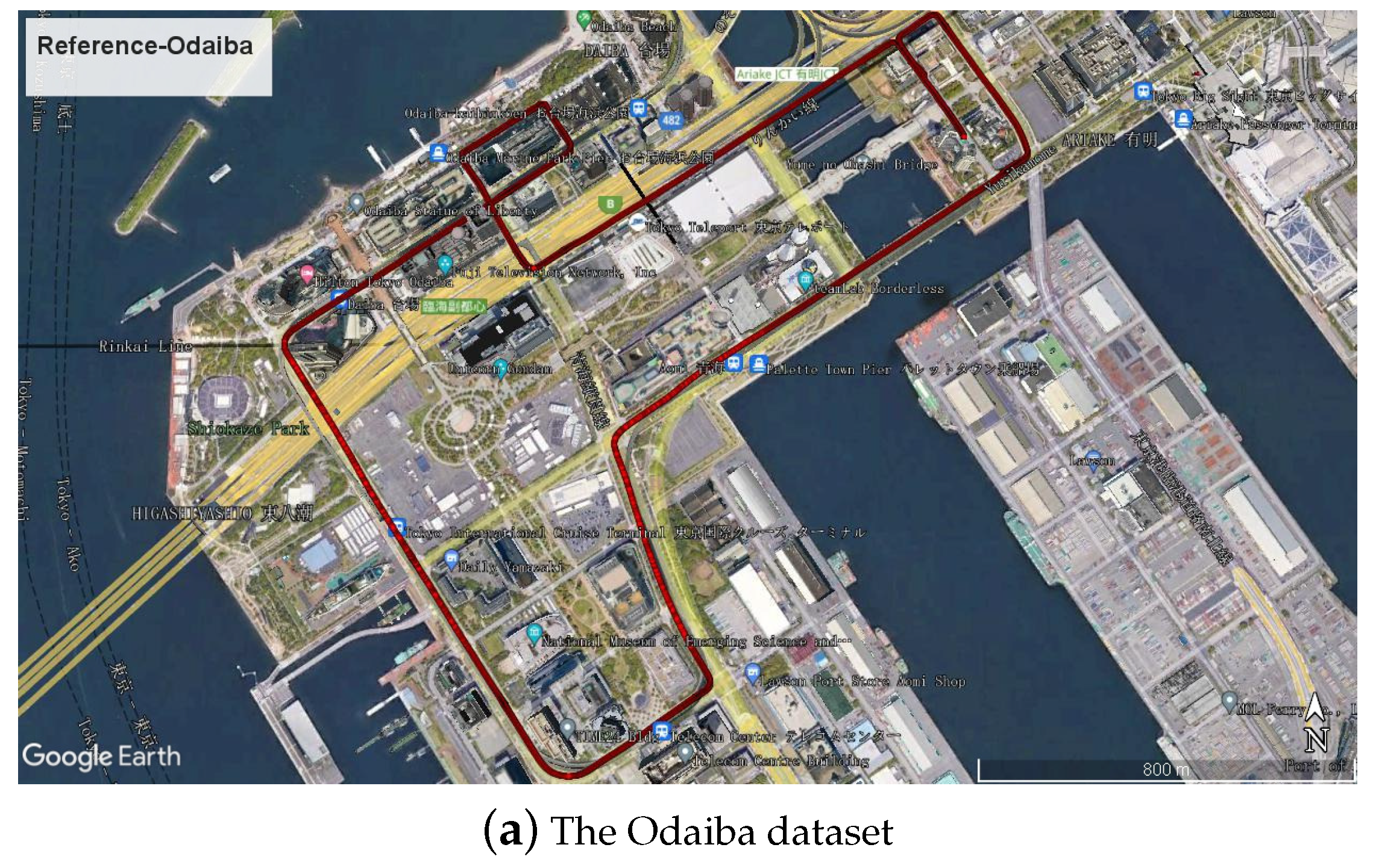
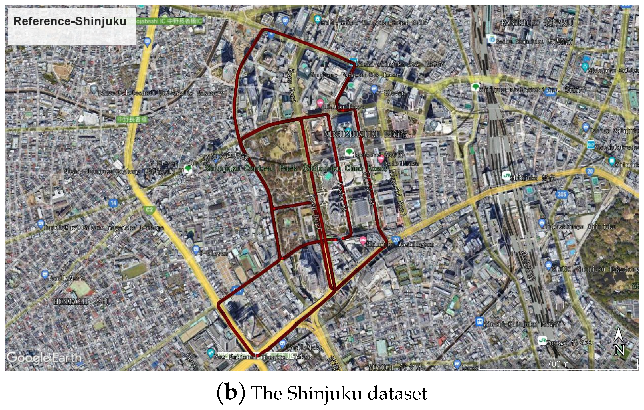
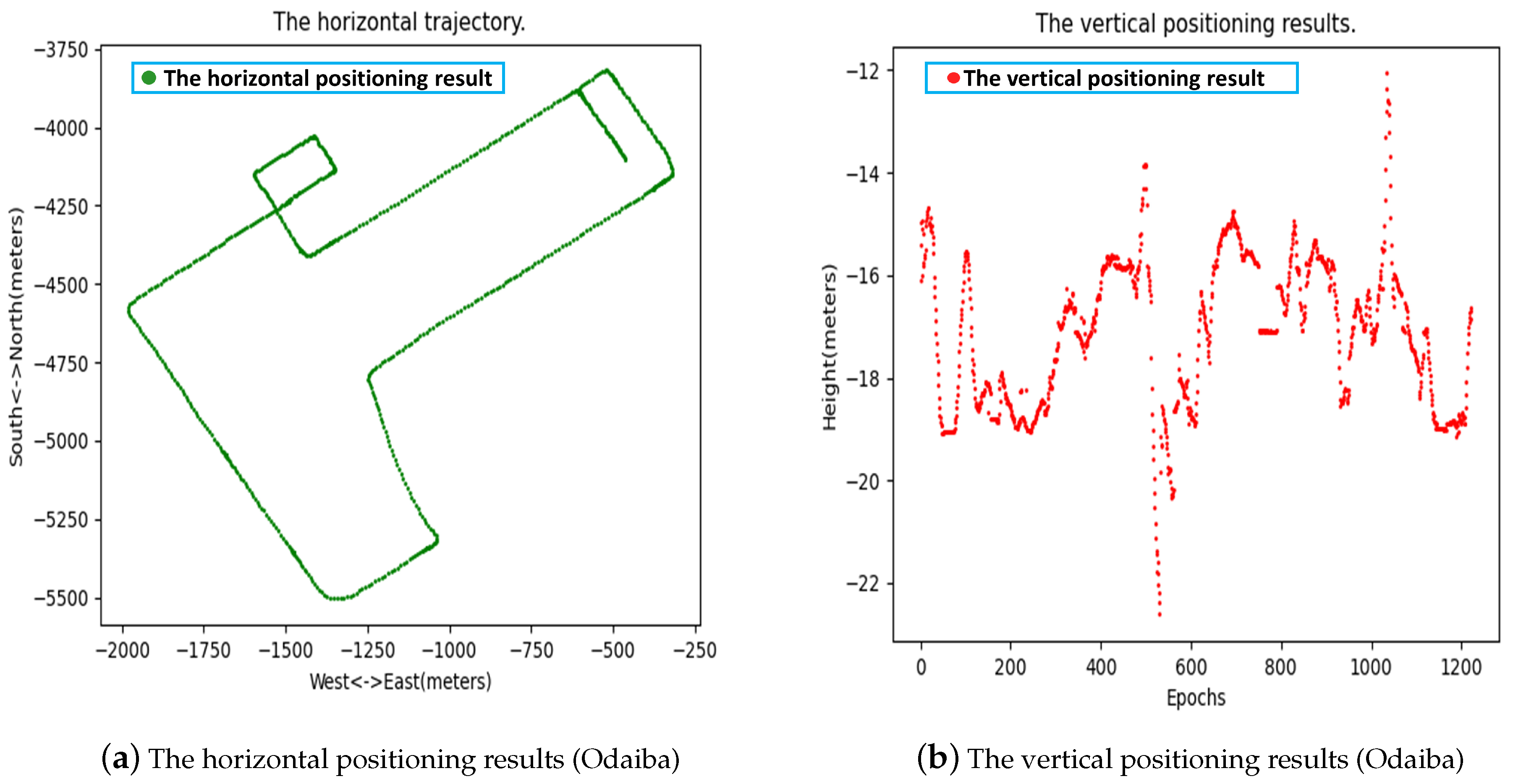
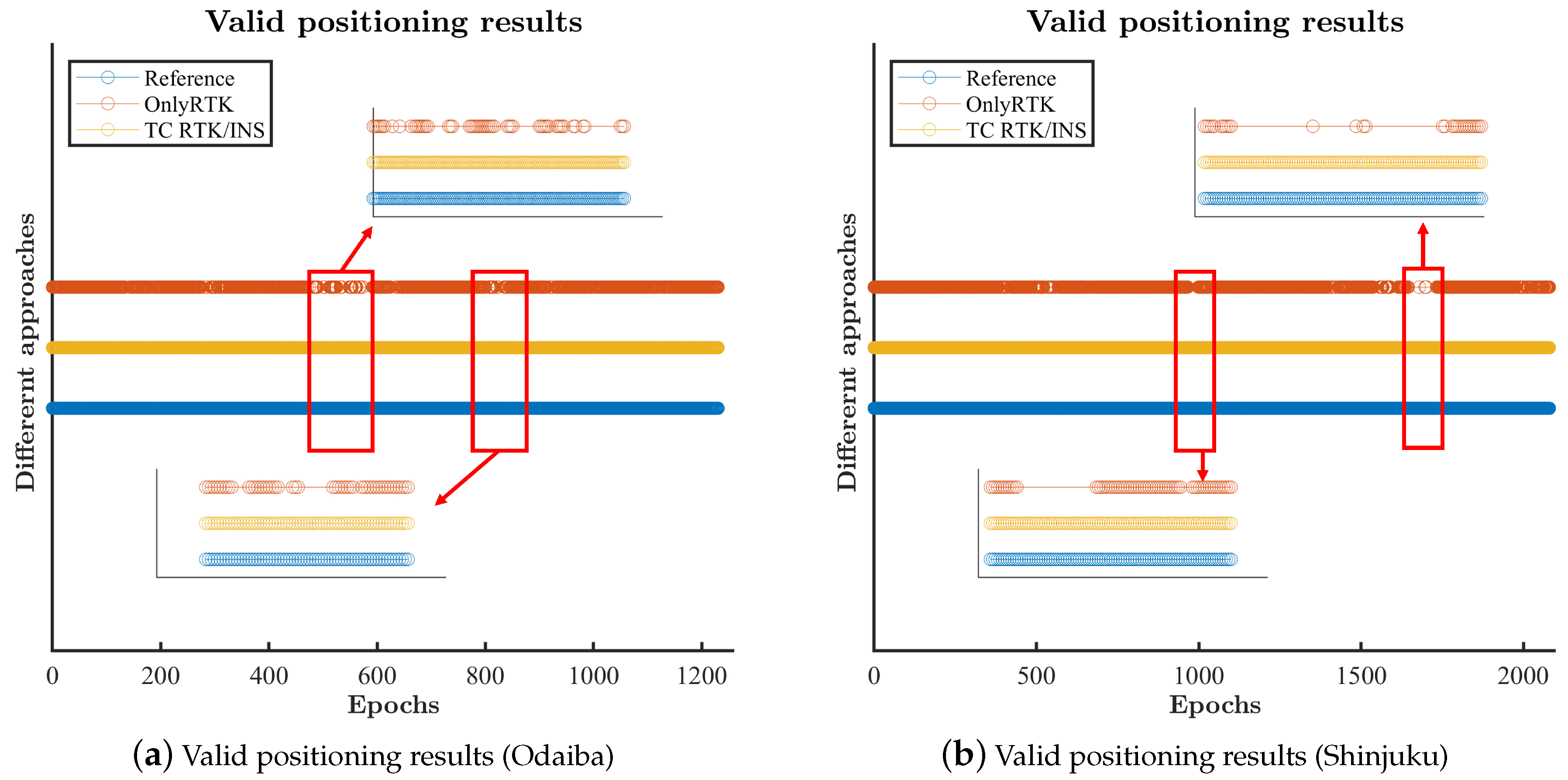
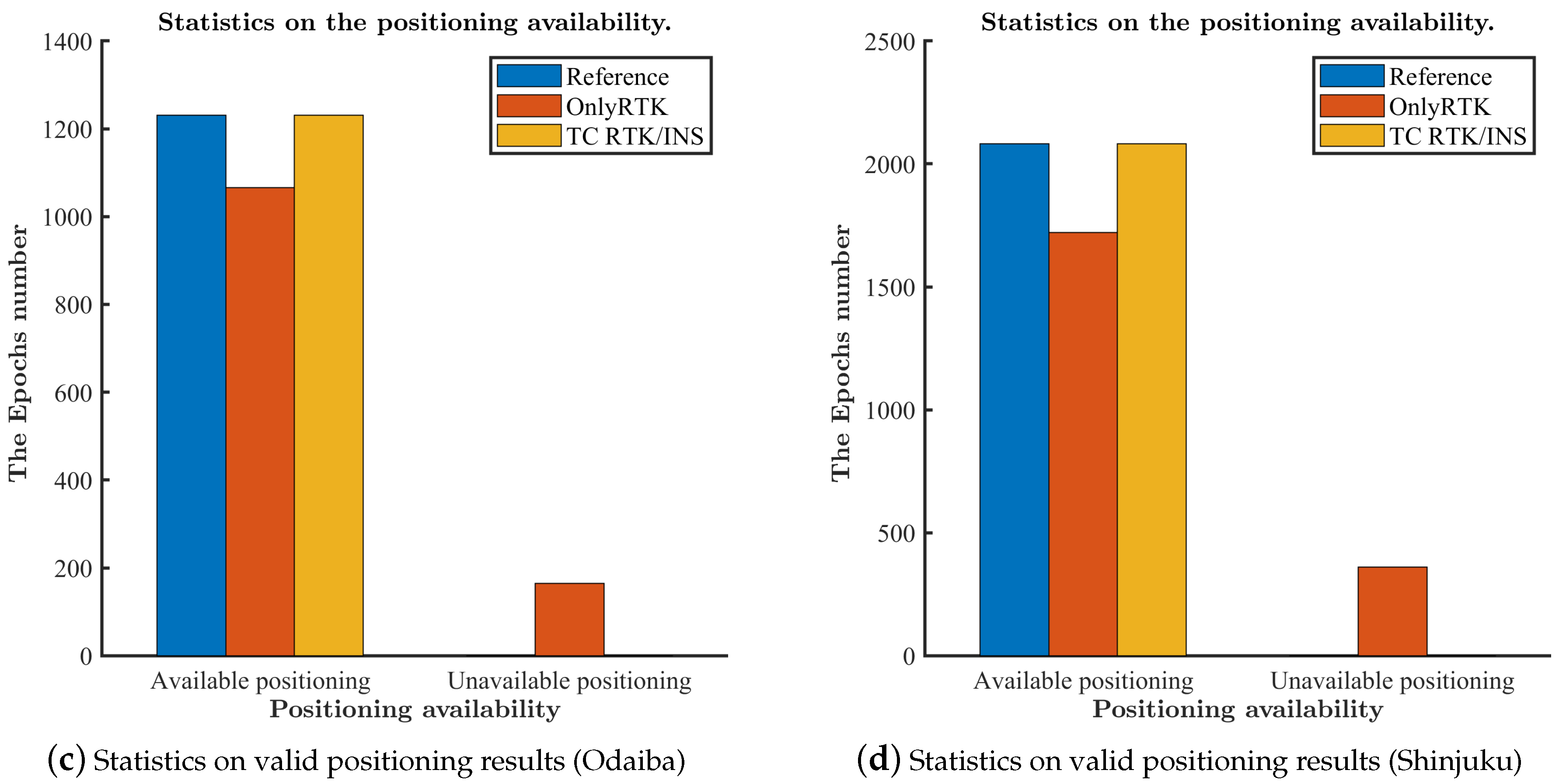
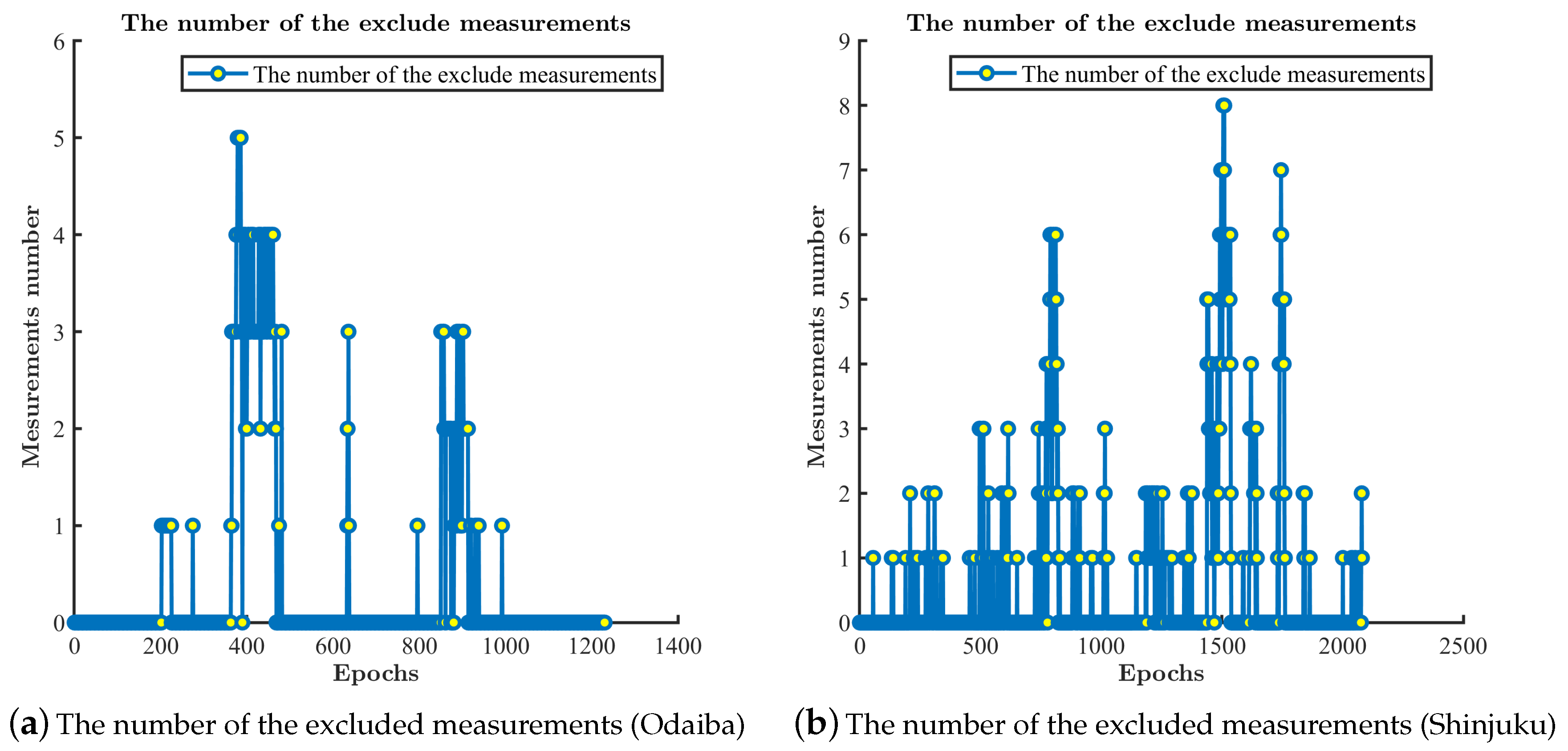
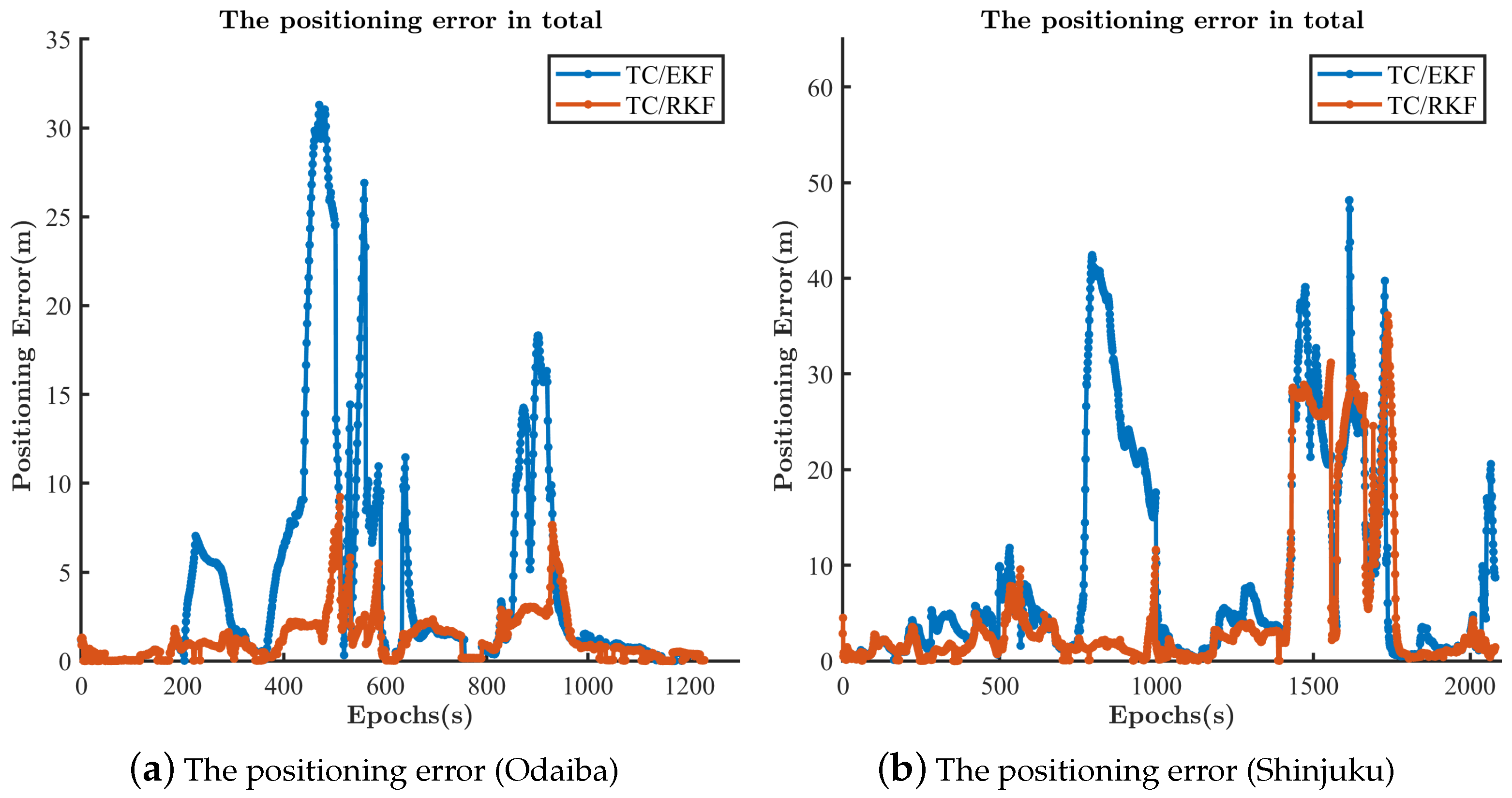
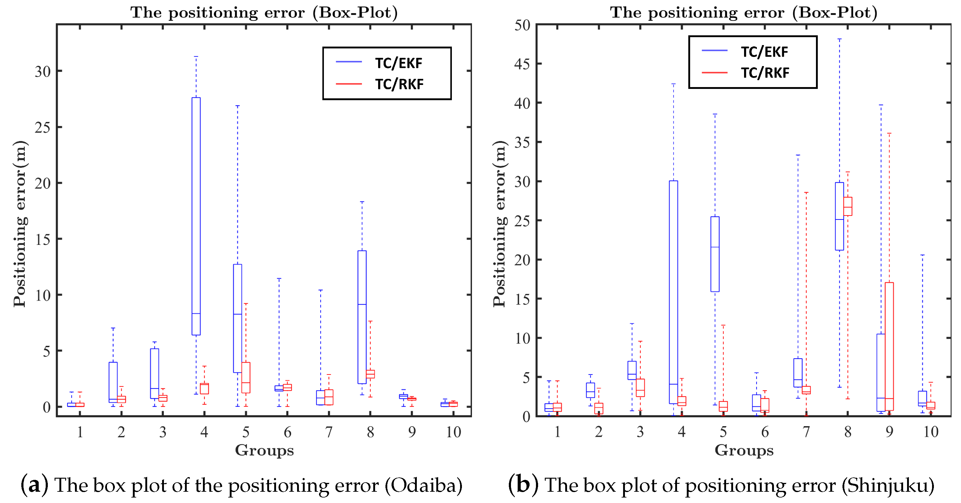
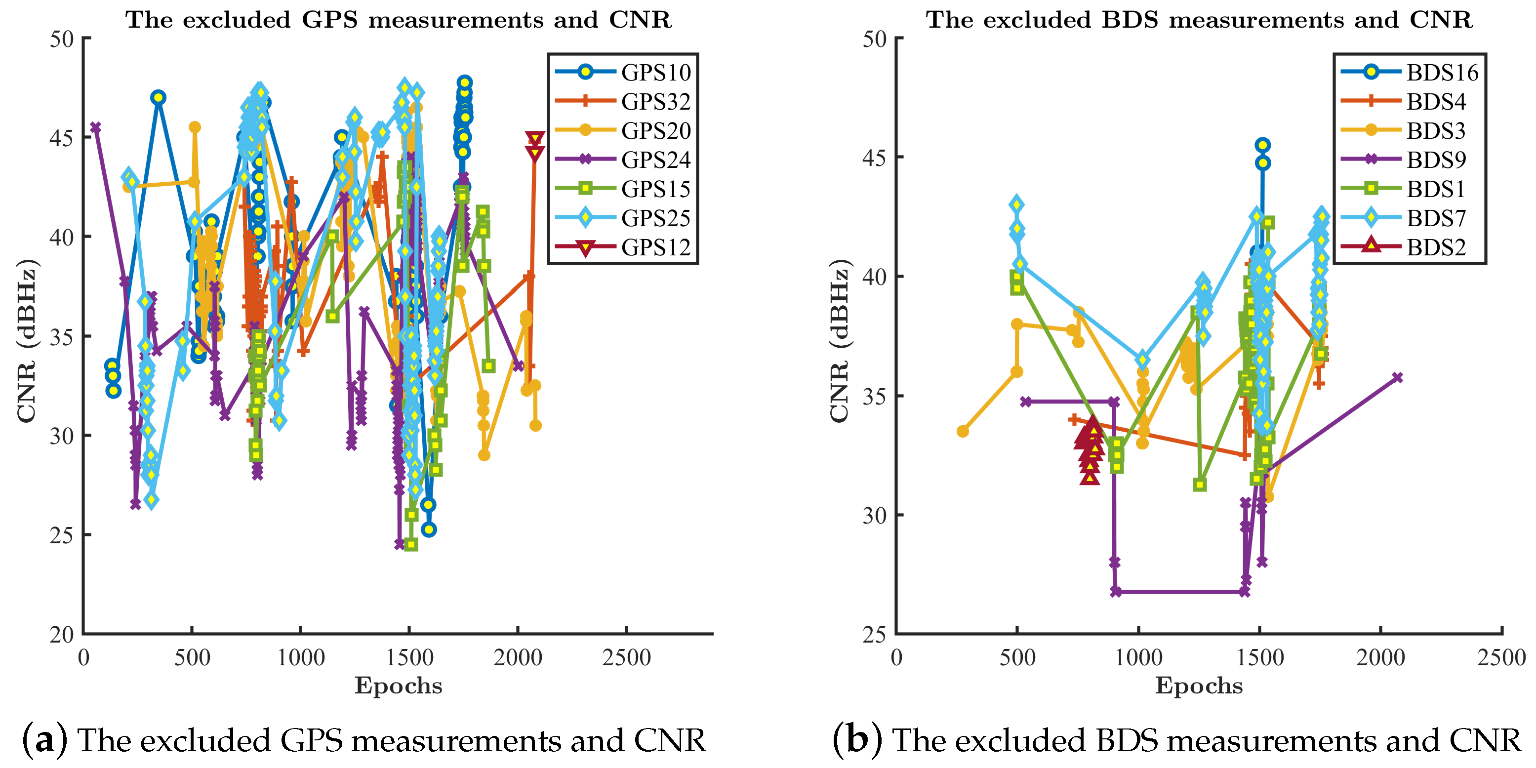
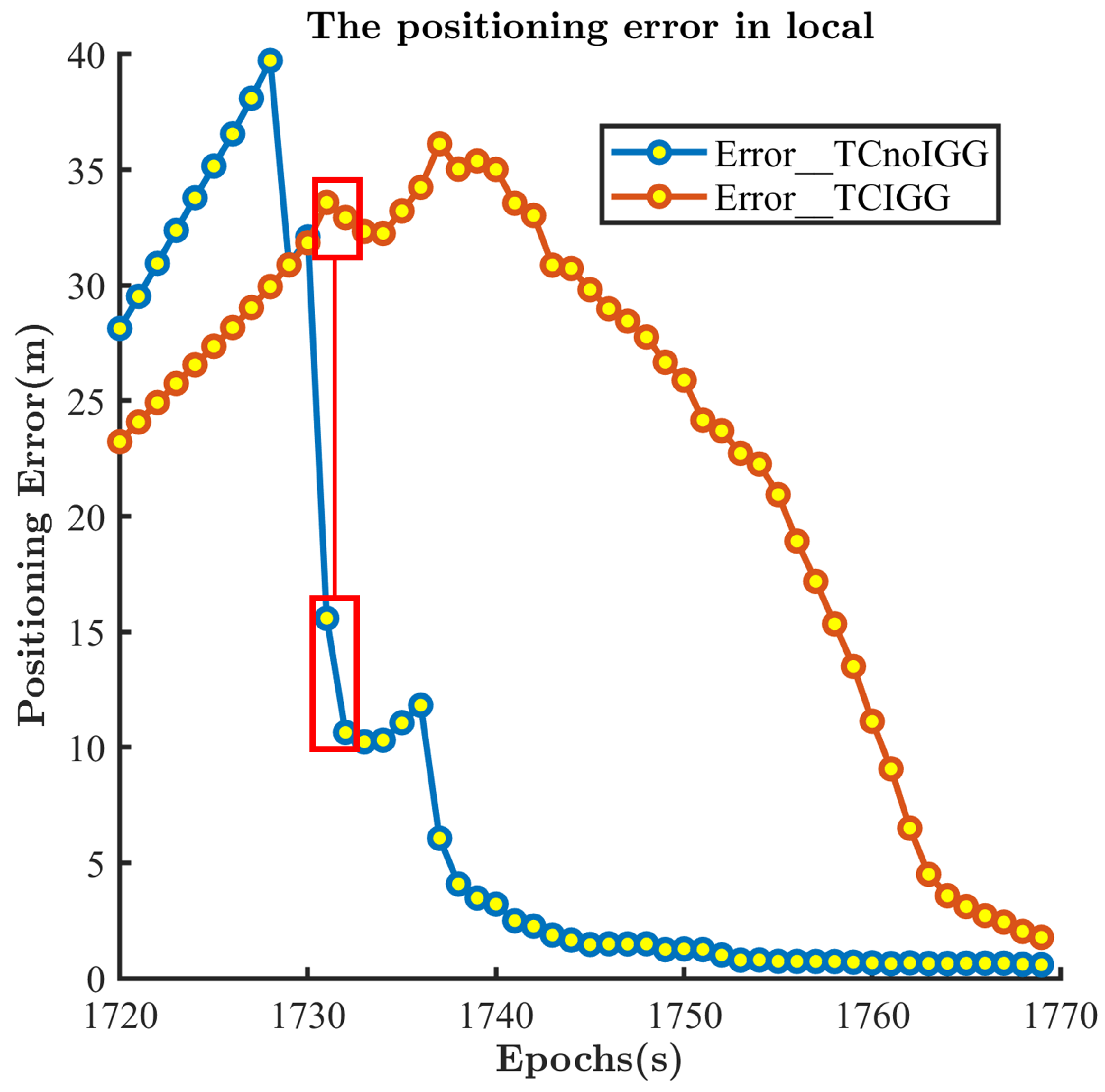
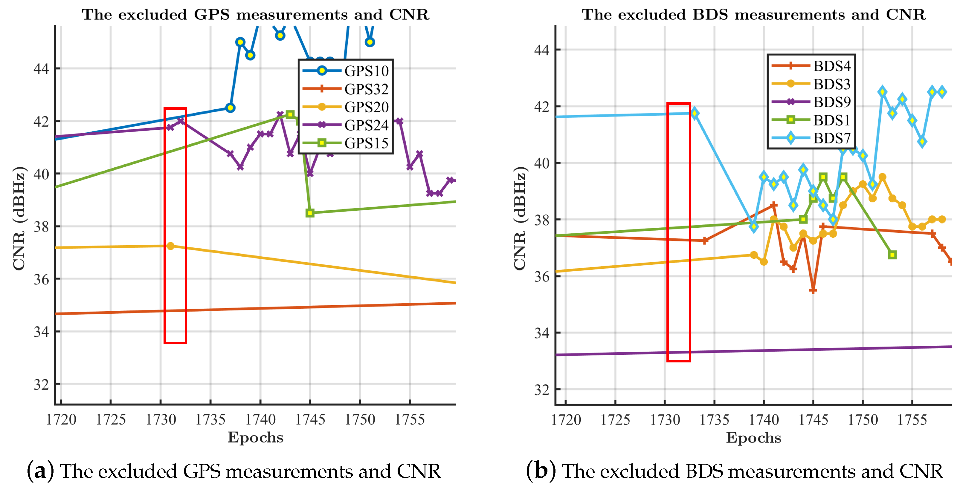
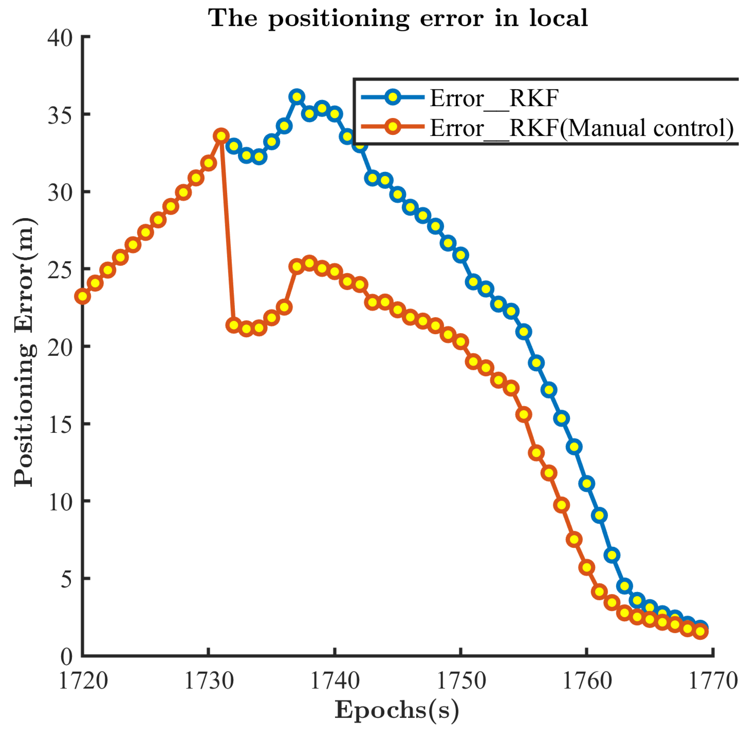
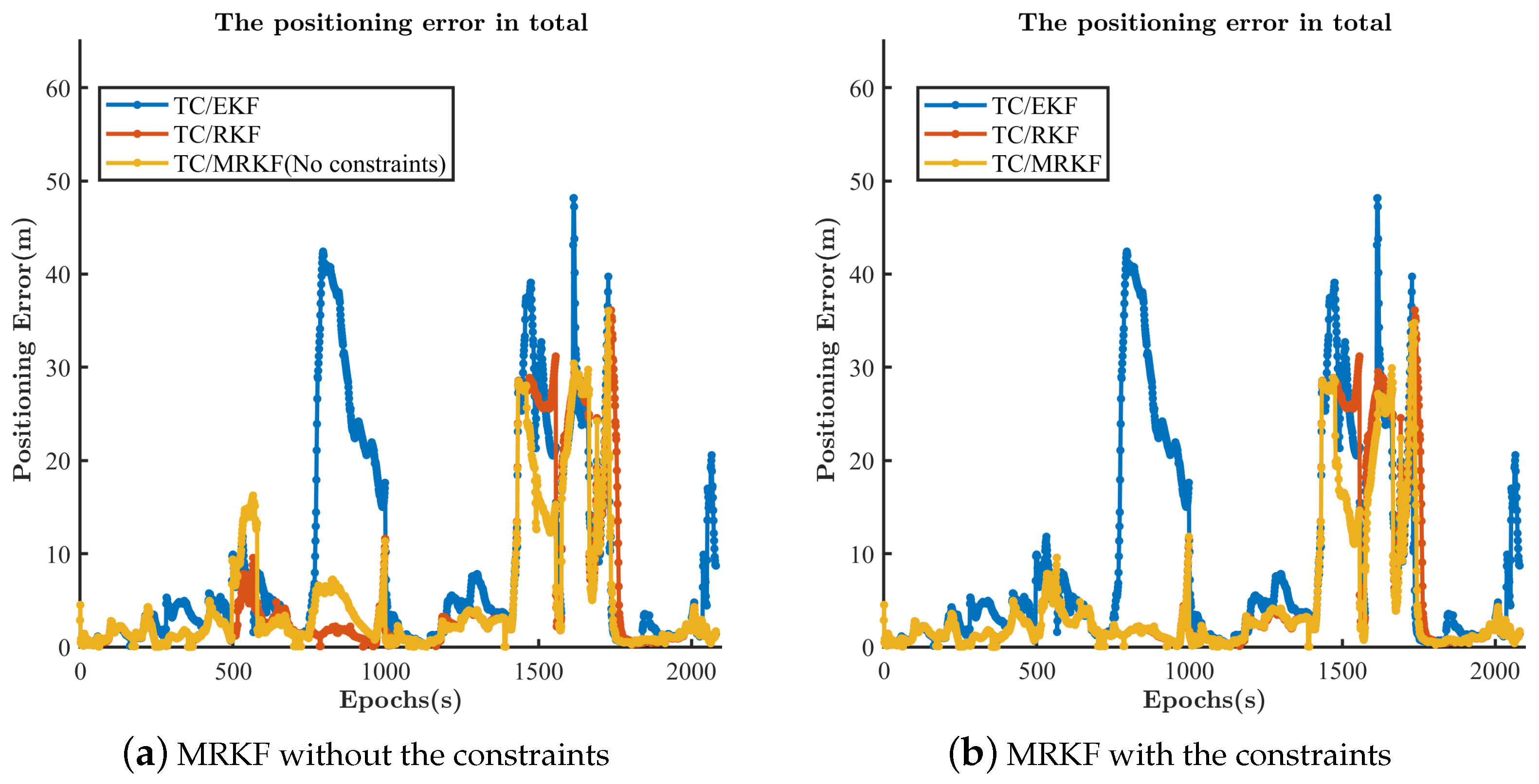
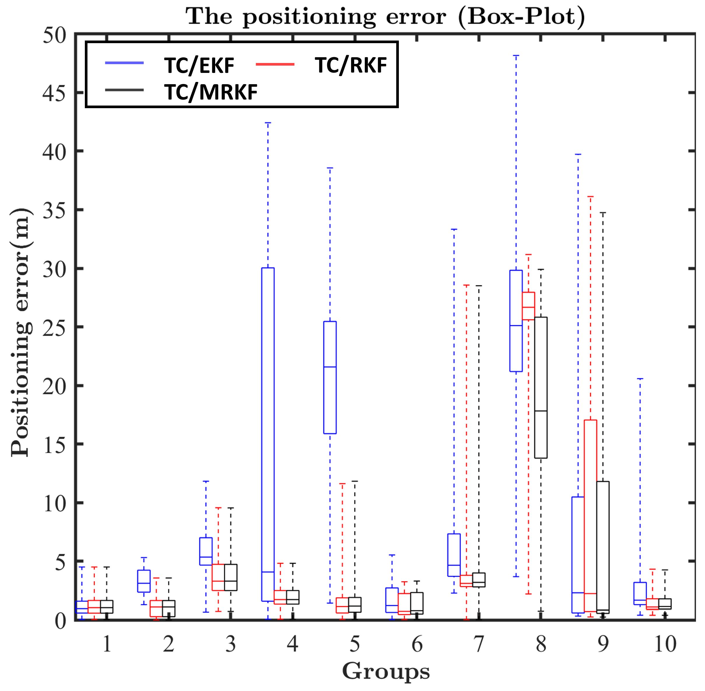
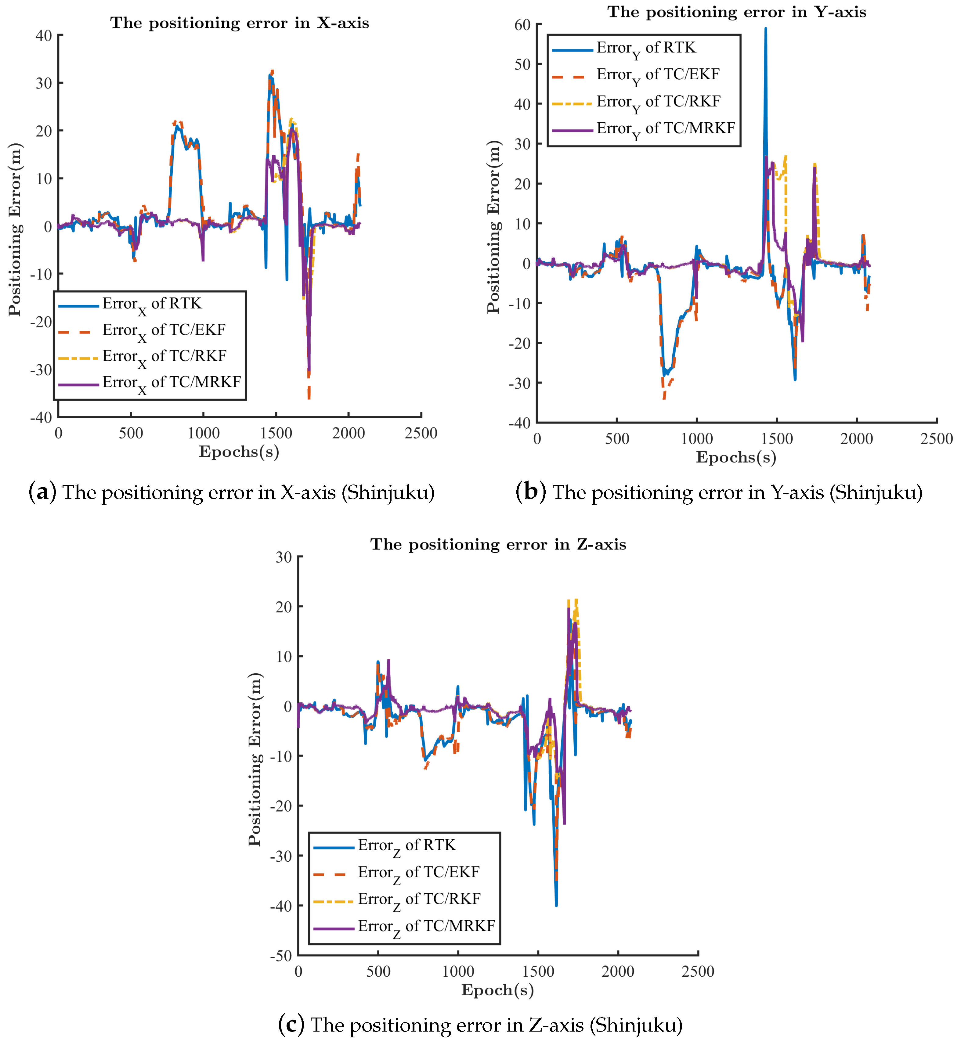
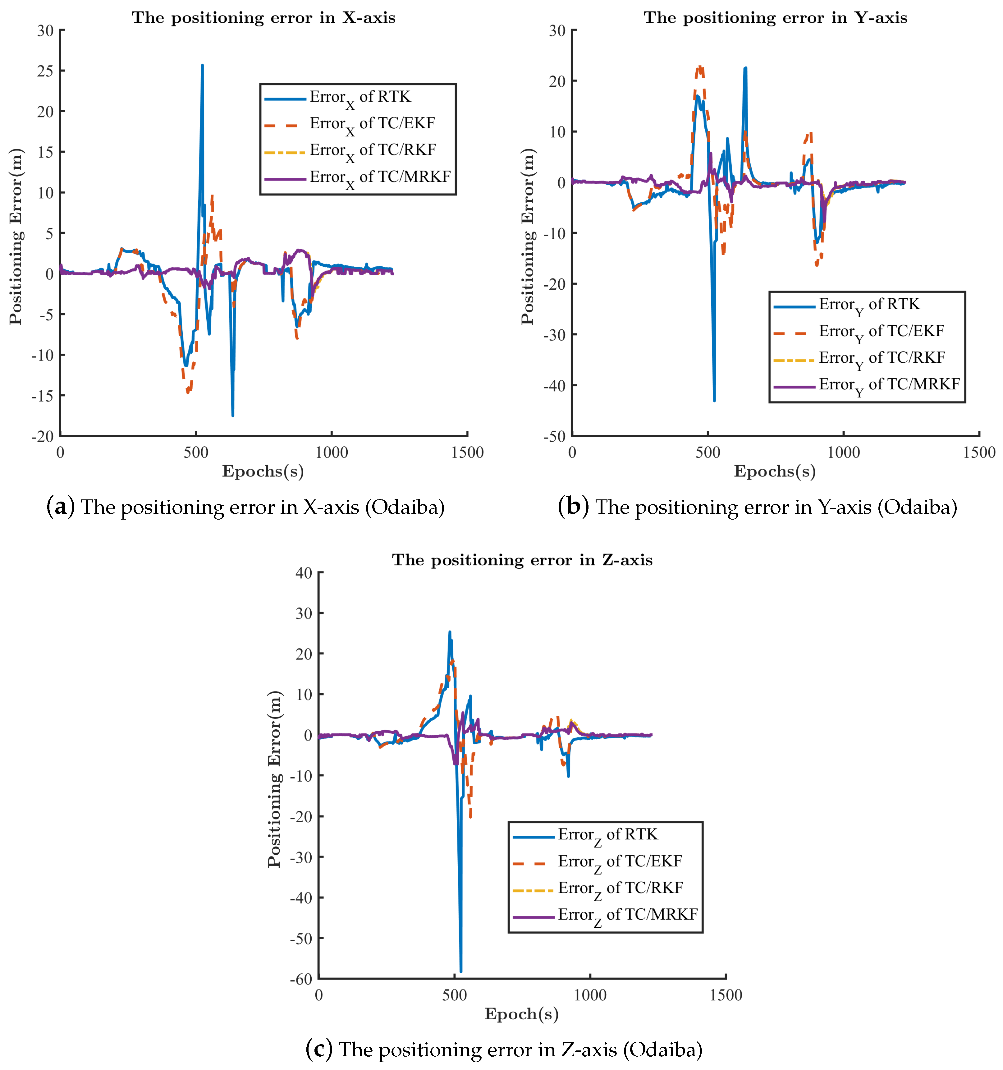
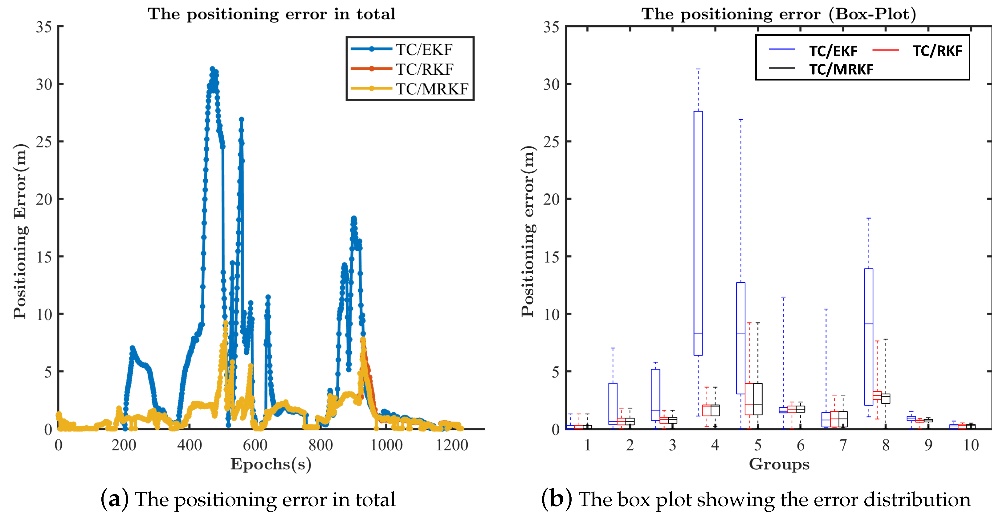
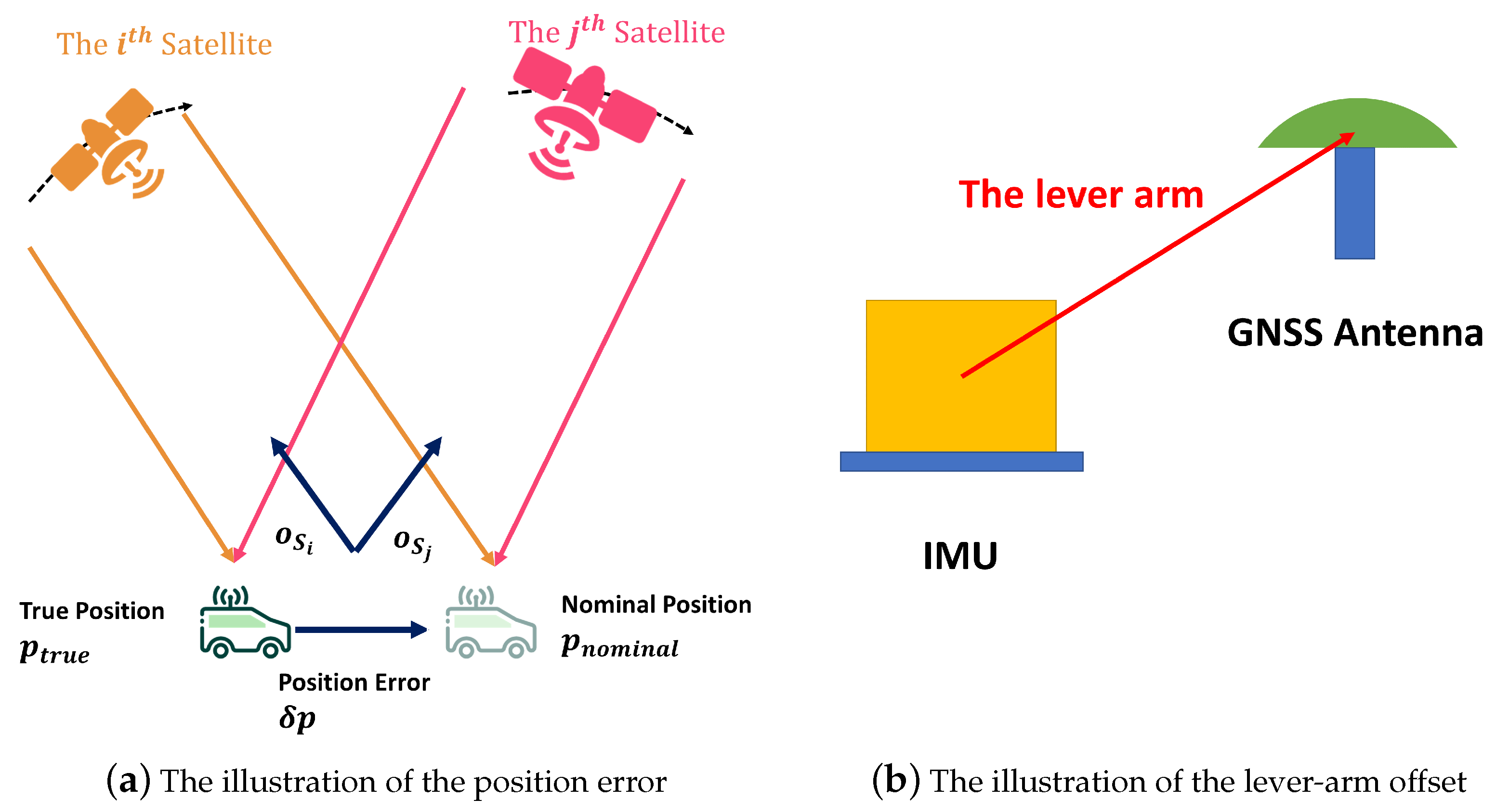
Table 1.
The characteristics of three integration strategies.
| Strategies | LC | TC | DC | |
|---|---|---|---|---|
| Characteristics | ||||
| EKF measurements | GNSS outputs (position and velocity) | Raw observations (pseudo range, phase, Doppler) | Loop parameters (code error, phase error) | |
| Minimum number of available satellites | Four | One | One | |
| Aiding receiver | No | No | Yes | |
| Acquisition and tracking performance improvement | No | No | Yes | |
| Disturbance resistance | No | No | Yes | |
| Cost and complexity | Low | High | Highest | |
| Possible to use INS to exclude outlying measurements | No | Yes | Yes | |
Table 2.
The characteristics of open-source projects.
| characteristics | Field | Frame | Language | |
|---|---|---|---|---|
| Projects | ||||
| RTKLIB | GNSS (RTK and PPP) | EKF | C | |
| PPPLIB | GNSS (RTK and PPP) GNSS/INS (LC) | EKF | C/C++ | |
| PSINS | GNSS/INS (LC and range-based TC) | EKF | Matlab/C++ | |
| GINAV | GNSS/INS (LC, range-based TC, PPK TC, PPP TC) | EKF | Matlab | |
| OB-GINS | GNSS/INS (LC) | Optimization | C++ | |
Table 3.
The outputs cases.
| Situation | Valid GNSS Measurements | AR | Generation | |
|---|---|---|---|---|
| Outputs | ||||
| Fixed Solution | Yes | Yes | Feedback to the float solution | |
| Float Solution | Yes | No | EKF estimation and feedback to the INS solution | |
| INS Solution | No | No | The INS mechanization | |
Table 4.
The positioning performance comparison (Odaiba).
| Techniques | RMSE (m) | Continuity | The Fixed Rate |
|---|---|---|---|
| RTK | 7.99 | 86% | 20% |
| TC RTK/INS (EKF) | 7.95 | 100% | 26% |
| TC RTK/INS (RKF) | 1.75 | 100% | 27% |
Table 5.
The positioning performance comparison (Shinjuku).
| Techniques | RMSE(m) | Continuity | The Fixed Rate |
|---|---|---|---|
| RTK | 13.21 | 82% | 10.0% |
| TC RTK/INS (EKF) | 14.17 | 100% | 12.8% |
| TC RTK/INS (RKF) | 10.01 | 100% | 13.1% |
Table 6.
The positioning performance comparison between four techniques (Shinjuku).
| Techniques | RMSE-X (m) | RMSE-Y (m) | RMSE-Z (m) | Total RMSE (m) | Fixed Rate |
|---|---|---|---|---|---|
| RTK | 8.95 | 8.07 | 5.43 | 13.21 | 10.0% |
| TC RTK/INS (EKF) | 9.70 | 8.44 | 5.94 | 14.17 | 12.8% |
| TC RTK/INS (RKF) | 5.49 | 6.92 | 4.70 | 10.01 | 13.1% |
| TC RTK/INS (MRKF) | 5.44 | 4.83 | 3.91 | 8.26 | 13.8% |
Table 7.
The positioning performance comparison between four techniques (Odaiba).
| Techniques | RMSE-X (m) | RMSE-Y (m) | RMSE-Z (m) | Total RMSE (m) | Fixed Rate |
|---|---|---|---|---|---|
| RTK | 3.25 | 5.00 | 5.31 | 7.98 | 20.0% |
| TC RTK/INS (EKF) | 3.58 | 5.58 | 4.39 | 7.95 | 26.1% |
| TC RTK/INS (RKF) | 0.90 | 1.08 | 1.19 | 1.84 | 26.8% |
| TC RTK/INS (MRKF) | 0.88 | 1.08 | 1.14 | 1.80 | 26.9% |
Publisher’s Note: MDPI stays neutral with regard to jurisdictional claims in published maps and institutional affiliations. |
© 2022 by the authors. Licensee MDPI, Basel, Switzerland. This article is an open access article distributed under the terms and conditions of the Creative Commons Attribution (CC BY) license (https://creativecommons.org/licenses/by/4.0/).
Share and Cite
MDPI and ACS Style
Niu, Z.; Li, G.; Guo, F.; Shuai, Q.; Zhu, B. An Algorithm to Assist the Robust Filter for Tightly Coupled RTK/INS Navigation System. Remote Sens. 2022, 14, 2449. https://0-doi-org.brum.beds.ac.uk/10.3390/rs14102449
AMA Style
Niu Z, Li G, Guo F, Shuai Q, Zhu B. An Algorithm to Assist the Robust Filter for Tightly Coupled RTK/INS Navigation System. Remote Sensing. 2022; 14(10):2449. https://0-doi-org.brum.beds.ac.uk/10.3390/rs14102449
Chicago/Turabian StyleNiu, Zun, Guangchen Li, Fugui Guo, Qiangqiang Shuai, and Bocheng Zhu. 2022. "An Algorithm to Assist the Robust Filter for Tightly Coupled RTK/INS Navigation System" Remote Sensing 14, no. 10: 2449. https://0-doi-org.brum.beds.ac.uk/10.3390/rs14102449
Note that from the first issue of 2016, this journal uses article numbers instead of page numbers. See further details here.