Retrieval of the Leaf Area Index from MODIS Top-of-Atmosphere Reflectance Data Using a Neural Network Supported by Simulation Data

Abstract

The leaf area index (LAI), a key parameter used to characterize the structure and function of the vegetation canopy, is crucial to simulations of the carbon, nitrogen, and water cycles of Earth’s system. In this paper, a neural network (NN) method coupled with vegetation canopy and atmospheric radiative transfer (RT) simulations is proposed to realize LAI retrieval without prior data support and complex atmospheric corrections. The look-up table (LUT) of the top-of-atmosphere (TOA) reflectance and associated input variables was simulated by 6S (6S simulation) based on the top-of-canopy (TOC) reflectance LUT simulated by PROSAIL. This was then used to train the NN to obtain the LAI inversion model. This method has been successfully applied to MODIS L1B data (MOD021KM), and the LAI retrieval of the vegetation canopy was realized. The estimated LAI was compared with the MODIS LAI (MOD15A2H) using mid-latitude summer data from 2000 to 2017 in the DIRECT 2.0 ground database. The experiments indicated that the LAI retrieved by the TOA reflectance (r = 0.7852, RMSE = 0.5191) was not much different from the LAI retrieved by the TOC reflectance (r = 0.8063, RMSE = 0.7669), and the accuracy was better than the MODIS LAI (r = 0.7607, RMSE = 0.8239), which proves the feasibility of this method.

1. Introduction

Currently, satellite products offer the only effective way to reflect global vegetation change. Many methods have been developed to retrieve biophysical parameters from remote sensing data, such as the leaf area index (LAI), the fraction of absorbed photosynthetically active radiation (FAPAR), and the fraction of vegetation cover (FCOVER), which greatly contribute to the study of Earth’s ecosystems [1,2,3,4].

The area of vegetation leaves is often characterized by the LAI, which is typically defined as one-half of the total area of green leaves per unit of horizontal ground surface area [5]. The LAI is an important vegetation structure parameter for the quantitative analysis of vegetation growth dynamics and biophysical processes, as well as a key input parameter for most climate, hydrology, biogeochemical, and ecosystem models [6]. In the carbon cycle, the LAI is a key factor that affects the ability of the canopy to absorb light and effective radiation, and this determines the photosynthetic capacity of the canopy and then affects the carbon cycle of an ecosystem [7]. In the water cycle, the LAI can change the evaporation of soil and surface water as well as the interception, accumulation, and transpiration of the canopy. In addition, it is significant in influencing the water and energy balance at the land surface [8]. Therefore, it is of great significance to obtain a large-scale, especially global-scale, LAI for simulating the response and feedback of the terrestrial ecological carbon system and water cycle to climate change [9].

LAI ground measurements are accurate, but they are time-consuming and labor-intensive, and one can typically only obtain the LAI at a small scale. Remote sensing technology has the advantages of wide coverage, high temporal and spatial resolution, and fewer ground restrictions. Therefore, for effective use in most global models of climate, biogeochemistry, and ecology, LAI products are routinely generated from remote sensing data [10,11]. Using the obtained canopy light radiation information to estimate the LAI provides a unique way to obtain the global LAI. A series of LAI products with different specifications have been produced based on satellite observation data, and these include MODIS LAI [12,13], CYCLOPES LAI [14], CCRS LAI [15], AVHRR LAI [16], ECOCLIMAP LAI [17], MISR LAI [18], POLDER LAI [19], GLASS LAI [20,21], CLOBCARBON LAI [22], and Copernicus LAI [23]. These LAI products have different spatial coverages and spatial resolutions, with temporal resolutions ranging from 4 days to 30 days and a time coverage from 1982 to present. The Moderate-Resolution Imaging Spectrometer (MODIS) reflectance data have the advantages of global coverage, strong timeliness, and high dynamics. They are advantageous for global phenology studies because of their higher revisit cycles and their ability to reflect the dynamic characteristics of vegetation growth and development. Therefore, the MODIS reflectance data play an important role in LAI inversion, vegetation growth status research, and global climate change [24,25]. In this paper, the daily LAI inversion is realized using the TOA reflectance data from MOD021KM based on single temporal data under clear sky conditions.

Several categories of methods can be used to estimate the LAI: empirical methods, physical methods, and NN methods [24]. The empirical methods are typically based on the statistical relationship between the LAI and various vegetation indexes (VIs) [26]. These methods are the most traditional methods and are simple and easy to implement and require few parameters. However, because remote sensing signals are multivariate nonlinear functions of surface and atmospheric parameters, there is no unified relationship between remote sensing observations and the LAI. Most of them need to use field measurements of the LAI and reflectance data recorded by a remote sensor or simulations from a canopy radiation model to calibrate for distinct vegetation types. Myneni et al. [27] proposed an atmospheric-corrected normalized difference vegetation index (NDVI) and constructed an LAI-NDVI relationship based on specific biological communities that was applied to AVHRR data and produced LAI datasets. Huete [28] proposed a soil-adjusted vegetation index (SAVI) that effectively reduced the influence of soil brightness on the VIs. In addition, a good linear relationship between the VI and LAI could be derived from the SAVI [29]. The empirical methods based on statistical relationships are generally applicable to specific vegetation types, sites, and times but lack an in-depth consideration of the radiation transfer mechanism. These methods are susceptible to various external factors, such as the atmosphere, the soil background, and sensor spectral bands, and, therefore, lack generality. It is worth mentioning that the empirical relationships can also achieve high accuracies for specific sites/dates/scenes.

The physical methods are mainly based on radiative transfer models to retrieve LAI. Because this approach is not limited by region and vegetation type and can be adjusted for a wide range of situations, radiative transfer models are increasingly used in the inverse mode to estimate the LAI from remotely sensed data [20,21]. Myneni et al. [6] developed an algorithm to retrieve the LAI from MODIS data based on a three-dimensional (3-D) radiative transfer model, and a global LAI product has been generated via this algorithm since 2000. Liu et al. [30] generated a 500 m forest LAI product with good reliability at an eight-day temporal resolution from 2000 to 2010. This was based on MOD09A1, MCD43A1 data, and a four-scale geometric optical model. These physical methods have a complete theoretical basis and can effectively express the process from biochemical parameters to remote sensing observations. They are based on the inversion of canopy radiative transfer models through LUT methods or other methods. However, physical models usually take vegetation canopy parameters (such as LAI, average leaf inclination), observation geometric parameters (such as solar zenith angle, observation zenith angle), single leaf reflectance and transmittance, and soil background reflectance as input parameters to simulate the bidirectional reflectance of a vegetation canopy. Therefore, the model itself is complex and needs a large number of input parameters; there may be great uncertainty in the final inversion results. This fact makes it difficult to meet the demand for high-precision LAI inversion in limited sensor bands. In addition, it is worth noting that these models also have limitations and require simplifications and assumptions [31,32].

NNs are a computationally efficient machine learning method with good autonomous learning and data mining capabilities. They can approximate complex nonlinear functions efficiently and accurately. The development of NNs allows ecologists to apply NN methods more easily to resolve the complexity of relationships between variables in ecological data. Therefore, these methods have great importance in ecological modeling [33]. They are increasing being used to estimate the LAI from remote sensing data [34]. In view of this, Baret et al. [14] used the SAIL + PROSPECT model to simulate the relationships between different biome variables, and they trained it by using NNs to produce global CYCLOPES LAI products based on radiometric calibrated data from the VEGETATION sensor. Masemola et al. [35] trained an artificial NN (ANN) based on the simulation dataset generated by the PROSAIL model, and the retrieved LAI had better accuracy than the LUT methods. All of the above are LAI inversion methods based on NNs. Strictly speaking, NN methods belong to a kind of physical methods, which are methods developed on the basis of the database simulated by the physical models. Firstly, a training sample database is constructed by using a physical model, and then the relationship between the input variables and the simulated canopy spectral values in the database is constructed by NN (that is, the construction of an LAI inversion model). Using this relationship, the canopy parameters can be calculated according to the observed canopy spectral information. Due to the complexity of the physical model, it is usually impossible to obtain its analytical solution, and the canopy and leaf variables must be solved by means of a numerical solution, and the NN method is one of the commonly used numerical solution techniques. In addition, the operation of these methods requires preprocessing remote sensing data to obtain the TOC reflectance data, which are then used to estimate biophysical variables. Therefore, we also refer to these approaches as TOC approaches.

To avoid complicated atmospheric correction processes, many researchers have proposed to invert the LAI based on the TOA reflectance data. Smith [36] used three bands (TM2, TM3, TM4) of reflectance from the Landsat TM without atmospheric correction to retrieve the LAI with the help of a back propagation (BP) NN. He obtained LAI inversion results with a higher accuracy than the statistical model methods. Fang and Liang [37] developed an NN algorithm to retrieve the LAI from Landsat-7 enhanced thematic mapper (ETM+) data, and they explored two schemes based on the surface reflectance and the TOA radiance, both of which accurately estimated the LAI. Furthermore, they found that bands 3 and 4 were more suitable for estimating the LAI from the ETM+ surface reflectance, while band 4 and the NDVI were more suitable if the TOA radiance was used. Estévez et al. [38] used the bottom of atmosphere (BOA) reflectance simulated by PROSAIL and the TOA reflectance further simulated by the 6SV model to train the variational heteroskedastic Gaussian process regression (VHGPR) model. They presented a computationally efficient approach of retrieving multiple crop traits (C_ab, C_w, FVC, LAI, LAI ∗ C_ab, LAI ∗ C_w) from Sentinel-2 data. It was found that, for leaf biochemicals, retrieval from the BOA reflectance slightly outperformed the results from the TOA reflectance. However, for most of the canopy-level variables, the estimation accuracy was higher when using the TOA reflectance data.

Considering the above, the primary objective of this study is to develop a retrieval workflow for estimating the LAI from the TOA reflectance data. Although there have been studies attempting to retrieve surface parameters from the TOA reflectance or radiance, the majority of the LAI retrievals have utilized the TOC reflectance. The obvious rationale behind this is to obtain the correct surface reflectance by removing atmospheric effects. To ensure successful retrieval of the LAI from TOA data, a good understanding of the atmospheric processes is required. Consequently, the TOA retrieval methods often rely on the coupling of a vegetation RTM with an atmospheric RTM. The atmosphere RTMs are used to model the atmospheric effects on the radiance emitted by a surface. In our study, the PROSAIL+6S RTMs were coupled to achieve the TOA retrieval of the LAI, and these RTMs were chosen for their simplicity and public availability. First, a LUT containing TOC reflectance, observation geometry, and LAI was simulated using the PROSAIL model [39]. Then, the 6S model was used for simulation and calculation to obtain the LUT about the TOA reflectance. After normalizing the simulated data, the deep belief network (DBN) was used for training to retrieve the LAI of different biomes. The input data used in our study were the MODIS TOA reflectance without atmospheric correction. To demonstrate the validity of our approach, the developed model was applied to the MODIS TOA reflectance and compared with a retrieval model applicable for the MODIS TOC reflectance data. In addition, it was also compared with the MODIS LAI and the ground-measured LAI. Among these, the MOD021KM data [40] provided the TOA reflectance, the MOD03 data [41] provided the geometric information of satellite observations, and the DIRECT 2.0 ground database [42] provided the ground-measured LAI. All the MODIS data used were data from 2000 to 2017. The retrieval workflow in our study does not require prior knowledge (such as land cover type), and, when applied to other sensors, only the spectral response function (SRF) in the retrieval workflow needs to be modified. In addition, we used the deep learning (DL) method based on DBN to determine the intrinsic regularity of the training data. This method can maximize the information mining of input data and deeply mine the internal relationship between LAI and other parameters. Therefore, DBN was applied to LAI retrieval to mine the vegetation information carried in the satellite signal as much as possible in this paper. Through experiments, it was found that, in addition to using the red and near infrared (NIR) bands with strong vegetation sensitivity, the inversion results are the best after introducing the green band and blue band (therefore, the vegetation information of MODIS 1-7 bands was used). This approach is a good choice for sensors that do not provide atmospheric correction datasets. In addition, the ideas in this paper are also applicable to retrieving other vegetation biochemical parameters, such as chlorophyll, FAPAR, and FVC.

In the following sections, we first describe the data acquired (Section 2.1) and introduce the method used (Section 2.2 and Section 2.3). In Section 3, we report the LAI inversion results and algorithm reliability checks. The performance of the method is discussed in Section 4, along with its advantages and limitations. Section 5 is the conclusion of our study.

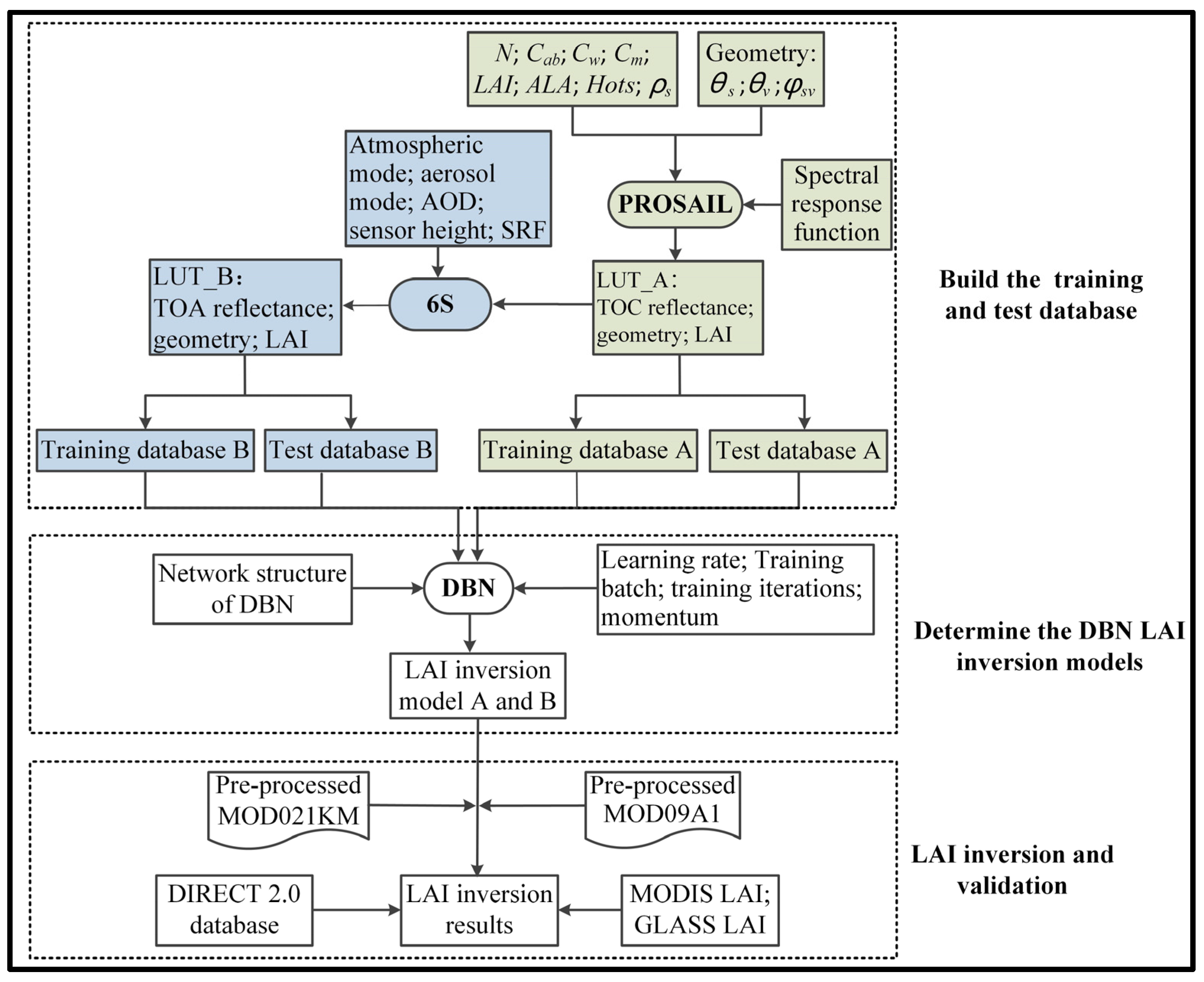
2. Materials and Methods

The retrieval method used in this study employed the DBN to estimate the LAI. First, the forward model (PROSAIL) was used to simulate the LUT_A of the TOC reflectance, observation geometry, and the LAI. Second, this LUT was used for the 6S simulation, and the LUT_B of the TOA reflectance, observation geometry, and LAI were calculated. Third, two LAI inversion models were obtained after training the DBN with these two simulated LUTs. The TOA reflectance of the MOD021KM 1–7 bands, the surface reflectance of the MOD09A1 1–7 bands, and the angle information (observed zenith angle, solar zenith angle, and relative azimuth) after being pre-processed were used as the input of the inversion models, and the output was the estimated LAI. A flow chart outlining this method is shown in Figure 1.

2.1. Satallite Data and Field Data

2.1.1. MODIS Data

The MODIS is a sensor mounted on the Terra and Aqua satellites that can acquire observational data in 36 discrete spectral bands ranging from 0.4 μm (visible light) to 14.4 μm (thermal infrared) [40,43]. Bands 1–7 cover the spectral information of red (620–670 nm), green (545–565 nm), blue (459–479 nm), and four NIR (841–876 nm, 1230–1250 nm, 1628–1652 nm, and 2105–2155 nm) bands, which can well reflect vegetation information.

The MODIS products used in this study included: MOD021KM (v6.1) [44], MOD03 (v6.1) [45], MOD09A1 (v061) [46], MCD12Q1 (v006) [47], and MOD15A2H (v061) [48]. The MOD021KM product primarily includes the image geographic location and radiometric calibration datasets, and these data can be used to calculate the TOA reflectance. The MOD03 product provides latitude and longitude coordinate data to assist MOD021KM in geometric correction. Both products have a time resolution of one day and a spatial resolution of 1 km. In this paper, the TOA reflectance data derived from the MOD021KM bands 1–7 were used. The MOD021KM data provided by the official website are the data after sensor calibration, and the conversion method from the original stored value of the image to radiance or TOA reflectance according to the gain and offset coefficients is shown in Equation (1). After radiometric calibration, the MOD021KM data need to be geometrically corrected with the latitude and longitude dataset in MOD03.

$$L_i=Scales\ast (SI-Offsets),$$

(1)

where $L_i$ represents the TOA radiance or the TOA reflectance after radiometric calibration, and $SI$ (scaled integers) represents an integer value that has been scaled.

The MOD09A1 product provides the surface reflectance (TOC reflectance) after atmospheric correction. The time resolution of this product is eight days, and the spatial resolution is 500 m, and these are provided to users in a sinusoidal projection system. The MOD09A1 provides reflectance data, which include: the red band, the blue band, the green band, and four NIR bands. It also provides the observation geometries that include: the solar zenith angle, the observation zenith angle, and the relative azimuth. The MOD09A1 data need to be preprocessed prior to using the reflectance of the seven bands. The downloaded data in the HDF-EOS (hierarchy data format—Earth Observation System) format are processed into the TIF (tag image file format) format, and the original digital number (DN) value is multiplied by a coefficient of 0.0001 to obtain the real surface reflectance. The equation used is shown in Equation (2).

$$\rho ={\rho }_0\times 0.0001,$$

(2)

where $\rho$ and ${\rho }_0$ represent the real surface reflectance value of a pixel and the original stored value on the image, respectively.

The MCD12Q1 product provides land cover type data with a temporal resolution of one year and a spatial resolution of 1 km to distinguish the different vegetation types when generating LAI maps [49]. The LAI legend (LC_Type3) of MCD12Q1 was used in this study. The LAI classification includes eight vegetation biomes (grasslands, shrublands, broadleaf croplands, savannas, evergreen broadleaf forests, deciduous broadleaf forests, evergreen needleleaf forests, deciduous needleleaf forests) and four other biomes (water bodies, non-vegetated lands, urban and built-up lands, unclassified). These eight vegetation biomes were combined into six biomes to facilitate comparison with the MODIS LAI. The evergreen broadleaf forests and deciduous broadleaf forests are combined into broadleaf forests, whereas evergreen needle forests and deciduous needle forests are combined into needle forests.

The MOD15A2H is a MODIS LAI product with a spatial resolution of 500 m and a temporal resolution of eight days that has been produced since 2002, and it is one of the most widely used LAI data sources at present. The MODIS LAI retrieval algorithm includes a primary algorithm and a backup algorithm [6,50]. The primary algorithm estimates the LAI based on LUT inversion. The input of the LUTs is the atmospherically corrected MODIS red and NIR surface reflectance (also referred to as the TOC reflectance in this paper) and the corresponding illumination-view geometries. The output of the LUTs is the mean LAI calculated over a set of acceptable LUT elements. When the primary algorithm fails, the backup algorithm is used to estimate the LAI based a on biome-specific LAI-NDVI empirical relationship [51]. Generally, the canopy structure and the leaf shape are unique in different biomes. Hence, the MODIS LAI retrieval algorithm uses the land cover product (MOD12Q1) as a priori information to constrain. Although this method can improve the retrieval speed, a land cover classification error is one of the biggest causes of LAI inversion uncertainty [24,25].

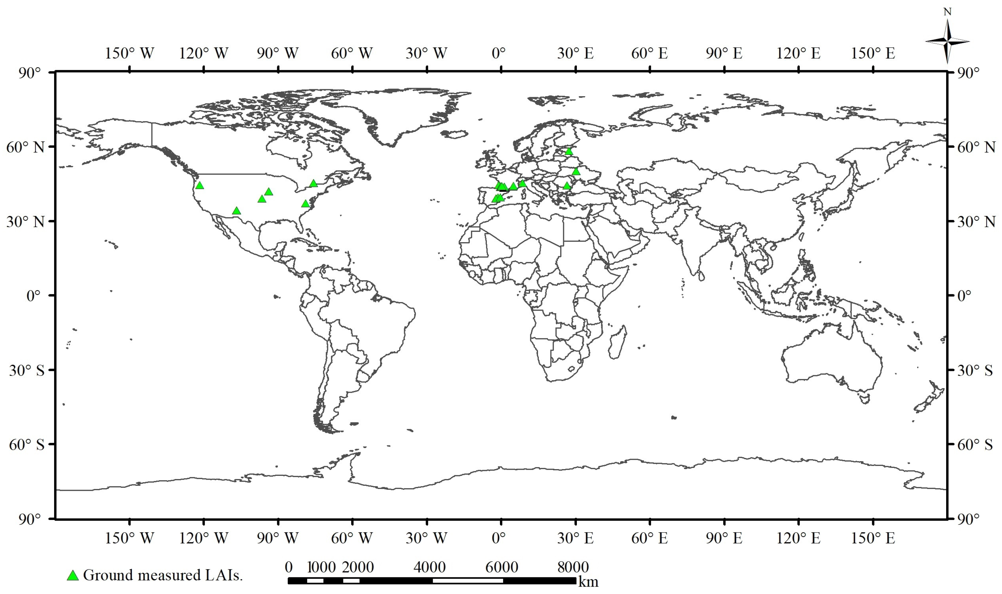
2.1.2. DIRECT 2.0 Ground Database

DIRECT 2.0 is a ground database of the LAI provided by the CEOS land product validation subgroup (LPV) that has been processed according to the CEOS-LPV guidelines [42]. It provides users with detailed information about the location, time, and LAI value (3 km × 3 km) of the measurement sites, and it is free for everyone to download and use. The authors of this database filtered forest sites without understory vegetation and extended the time series to 2017 [42] (https://calvalportal.ceos.org/web/olive/site-description, accessed on 28 September 2021). There are 242 field data of 140 ground sites in total from 2000 to 2017 (from FP7 ImagineS, VALERI, BigFoot, ESA, EOLAB, SAFARI, and CCRS).

The mid-latitude (latitude between 30–60) summer (June, July, and August) field data (50 mid-latitude summer LAI are available in the DIRECT 2.0 database) were selected to verify the algorithm used in this paper. Correspondingly, during the data simulation, the atmospheric mode parameter in the 6S model was designed to be the “mid-latitude summer”. These selected sites included different vegetation biomes, such as crops, shrubs, mixed forests, and needle-leaved forests. In order to ensure a spatiotemporal match between the field data and the different LAI products during verification, we selected LAI mean values of 3 km × 3 km from 2002 to 2017; the latitude, longitude, date, and average 3 km × 3 km LAI of the selected sites are shown in

Table 1. Information of the selected sites.

Site Name	Country	Lat	Lon	Land Cover	DOY	LAI	Reference
KONZ	USA	39.0890	−96.5712	Crops	2000159	2.175	BigFoot
Nezer	France	44.5680	−1.0375	NLF	2000211	1.591	VALERI
Fundulea	Romania	44.4060	26.5832	Crops	2002144	1.284	VALERI
Walnut_Creek	USA	41.9322	−93.7510	Crops	2002174	1.386	NAN
Walnut_Creek	USA	41.9322	−93.7510	Crops	2002182	2.145	NAN
Walnut_Creek	USA	41.9322	−93.7510	Crops	2002189	2.880	NAN
SudOuest	France	43.5063	1.2375	Crops	2002189	1.228	VALERI
Alpilles2	France	43.8104	4.7146	Crops	2002204	1.054	VALERI
SEVI	USA	34.3509	−106.6899	Shrubs	2002207	0.121	BigFoot
Appomattox	Canada	37.2183	−78.8838	Mixed F.	2002217	1.89	US EPA
SEVI	USA	34.3509	−106.6899	Shrubs	2002234	0.311	BigFoot
SEVI	USA	34.3509	−106.6899	Shrubs	2002252	0.402	BigFoot
METL	USA	44.4508	−121.5730	NLF	2002267	1.906	BigFoot
Fundulea	Romania	44.4060	26.5832	Crops	2003144	0.913	VALERI
SEVI	USA	34.3509	−106.6899	Shrubs	2003174	0.061	BigFoot
Barrax	Spain	39.0728	−2.1040	Crops	2003193	0.965	VALERI
SEVI	USA	34.3509	−106.6899	Shrubs	2003209	0.047	BigFoot
SEVI	USA	34.3509	−106.6899	Shrubs	2003258	0.05	BigFoot
Plan_De_Dieu	France	44.1987	4.9481	Crops	2004189	0.469	VALERI
Barrax	Spain	39.0728	−2.1040	Crops	2004196	0.553	VALERI
Barrax2	Spain	39.0281	−2.0743	Crops	2005194	0.267	EOLAB
Barrax	Spain	39.0728	−2.1040	Crops	2005194	0.27	VALERI
Utiel	Spain	39.5807	−1.2646	Crops	2006204	0.491	SMOS
Jarvselja	Estonia	58.2987	27.2623	Mixed F.	2007199	2.730	VALERI
Barrax	Spain	39.0728	−2.1040	Crops	2009173	0.558	VALERI
SouthWest_2	France	43.4471	1.1451	Crops	2013191	0.490	Imagines
SouthWest_1	France	43.5511	1.0889	Crops	2013191	0.810	Imagines
SouthWest_2	France	43.4471	1.1451	Crops	2013207	0.670	Imagines
SouthWest_2	France	43.4471	1.1451	Crops	2013230	1.620	Imagines
SouthWest_1	France	43.5511	1.0889	Crops	2013230	1.080	Imagines
SouthWest_2	France	43.4471	1.1451	Crops	2013247	1.790	Imagines
SouthWest_1	France	43.5511	1.0889	Crops	2013247	1.100	Imagines
Ottawa	Canada	45.3056	−75.7673	Crops	2014159	1.030	Imagines
Rosasco	Italy	45.2530	8.5620	Crops	2014184	2.620	Imagines
Ottawa	Canada	45.3056	−75.7673	Crops	2014187	1.820	Imagines
Pshenichne	Ukraine	50.0766	30.2322	Crops	2014212	2.010	Imagines
Barrax-LasTiesas	Spain	39.0544	−2.1007	Crops	2015147	0.740	Imagines
AHSPECT-MTO	France	43.5728	1.3745	Crops	2015173	0.550	Imagines
AHSPECT-URG	France	43.6397	−0.4340	Crops	2015174	1.390	Imagines
AHSPECT-PEY	France	43.6662	0.2195	Crops	2015174	0.900	Imagines
Pshenichne	Ukraine	50.0766	30.2322	Crops	2015174	1.370	Imagines
AHSPECT-CRE	France	43.9936	−0.0469	Crops	2015175	1.510	Imagines
AHSPECT-SAV	France	43.8242	1.1749	Crops	2015176	0.650	Imagines
AHSPECT-CON	France	43.9743	0.3360	Crops	2015176	0.770	Imagines
Pshenichne	Ukraine	50.0766	30.2322	Crops	2015188	1.860	Imagines
Pshenichne	Ukraine	50.0766	30.2322	Crops	2015204	1.470	Imagines
Barrax-LasTiesas	Spain	39.0544	−2.1007	Crops	2016194	0.464	Imagines
Moncada	Spain	39.5205	−0.3870	Crops	2017142	0.810	EOLAB
Moncada	Spain	39.5205	−0.3870	Crops	2017199	0.570	EOLAB

In the column of land cover, NLF = needle-leaved forests, Mixed F. = mixed forests. The “DOY” represents “day of year”, which is Julian day. The “LAI” represents the mean LAI of 3 km × 3 km.

. The selected sites include 39 crops sites, 2 mixed forests sites, 2 needle-leaved forests sites, and 6 shrub sites. The LAI values of these sites vary from 0.047 to 2.88. The spatial distribution of these sites is shown in Figure 2. We can see that some sites were relatively close to each other or overlapped; this was because the scale is too small, and the distance in Figure 2 was many times smaller than that in the field. Therefore, there was no apparent position difference between these sites.

2.2. Sample Data Simulation

Sufficient high-quality and representative sample data are an important prerequisite for the estimation of vegetation biochemical parameters using NN methods. Ideally, the sample data should represent all conditions that may be detected by the MODIS sensor. However, due to the complexity of the surface structure and the limited distribution of the current observation sites, it is difficult to obtain sufficient samples on a wide range of the different biomes. To solve this problem, we used the RT model simulation method. Based on real surface scenes, the possible surface scenes were established artificially. When simulating the training data, the PROSAIL model was first used to simulate the TOC reflectance of the MODIS 1–7 bands to generate the LUT_A containing the TOC reflectance, the solar zenith angle, the observation zenith angle, the relative azimuth, and the LAI. Then, 6S simulation was applied to calculate TOA reflectance and generate the LUT_B containing the TOA reflectance, three angles, and LAI. When these sample data were applied to the NNs for training, the input data were the MODIS reflectance data and geometry from the simulation data (LUT_A and LUT_B), and the output was the LAI.

2.2.1. Creation of the LUT with the PROSAIL Model

The PROSAIL model [52] was obtained by coupling the PROSPECT-5B and 4SAIL models and can be used to simulate the vegetation canopy reflectance with a spectral range from 400 to 2500 nm and a spectral resolution of 1 nm (Equation (3)). It can be seen from Equation (1) that the canopy reflectance is affected by multiple parameters. Therefore, a sensitivity analysis of each parameter should be conducted before setting. The value range of each parameter was determined according to the Leaf Optical Properties Experiment 93 (LOPEX93) database [53] and previous literature research [14,32,38,54], and a step length was set according to the sensitivity of each parameter to the vegetation canopy spectrum [39] (as shown in

Table 2. Parameter settings of the PROSAIL model.

Model	Parameter	Description	Unit	Step Length	Range
PROSPECT	N	Leaf structure	Unitless	0.5	1–4
	Cab	Chlorophyll concentration	μg cm−2	15	15–90
	Cw	Equivalent water thickness	cm	0.015	0.005–0.035
	Cm	Leaf dry matter content	g cm−2	0.01	0.001–0.03
	Car	Carotenoid content	μg cm−2	/	6
	Cbrown	Brown pigment content	Unitless	/	0.2
SAIL	LAI	Leaf area index	m2 m−2	0.2	0–7
	ALA	Mean leaf inclination	°	30	0–90
	${\rho }_S$	Soil brightness	Unitless	0.2	0–1
	Hots	Hot spot parameter	m m−1	0.03	0.01–0.1
	${\theta }_S$	Solar zenith angle	°	9	0–72
	${\theta }_v$	Sensor zenith angle	°	9	0–72
	${\phi }_{sv}$	Relative azimuth angle	°	15	0–180

).

$$\rho (\lambda )=\mathrm{PROSAIL}(N,C_{ab},C_w,C_m,C_{ar},C_{brown},\mathrm{LAI},Hots,ALA,skyl,{\rho }_S,{\theta }_S,{\theta }_v,{\phi }_{sv}),$$

(3)

where $\rho (\mathsf{\lambda })$ is the canopy reflectance at wavelength $\lambda$; N is the leaf structure parameter; C_ab is the chlorophyll a + b content; C_w is the equivalent water thickness; C_m is the dry matter content; C_ar is the carotenoid content; C_brown is the brown pigment content; LAI is the leaf area index; Hots is the hot spot parameter (ratio of the average leaf size to the crown height); ALA is the average leaf inclination; skyl is the ratio of the diffuse to the total incident radiation; ${\rho }_S$ is the soil brightness; ${\theta }_S$ is the solar zenith angle; ${\theta }_v$ is the sensor zenith angle; and ${\phi }_{sv}$ is the relative azimuth angle.

The TOC reflectance of the MODIS 1–7 bands in LUT_A was calculated from the canopy reflectance simulated by PROSAIL. The LUT of LAI-TOC reflectance was calculated by convoluting the canopy reflectance according to Equation (4) shown below.

$$R_i=\frac{{\displaystyle \sum _{j=j_0}^{j=j_n}\rho ({\lambda }_j)r_j}}{{\displaystyle \sum _{j=j_0}^{j=j_n}\rho ({\lambda }_j)}},$$

(4)

where $R_i$ is the is the TOC reflectance of band $i$ (the value of i is 1, 2, …, 7); $j$ is the wavelength range of band $i$; $j_0$ and $j_n$ are the minimum and maximum wavelengths of band $i$, respectively; $r_j$ is the SRF at the wavelength of $j$ nm; and $\rho ({\lambda }_j)$ is the canopy reflectance at $j$ nm as simulated by the PROSAIL model.

2.2.2. 6S Simulation

The 6S (second simulation of satellite signal in the solar spectrum) is probably the most widely used atmospheric correction code based on radiative transfer. It is an improved version of the 5S (simulation of satellite signal in the solar spectrum) proposed by Tanre et al. [55]. The improvement is that when calculating the scattering and absorption of the spectrum, the more advanced approximation algorithm and the successive order of the scattering algorithm are used to improve the accuracy of the Rayleigh scattering and aerosol scattering effects and simulate the atmospheric influence of sunlight on the transmission process of the “sun-ground target-sensor”. The spectral simulation range of 6S is 250–4000 nm, and the spectral resolution is 2.5 nm. The detailed information of the 6S algorithm is widely provided in the references [56,57,58,59,60], so it will not be introduced in this paper.

The calculation process of the 6S model is divided into a forward calculation and a reverse calculation. The forward calculation primarily refers to the simulated calculation of the TOA reflectance received by the satellite according to the input parameters, whereas the reverse calculation is a simulation of the TOC reflectance, that is, the process of atmospheric correction. In this paper, the forward calculation process was used. The LUT_A containing three angles and the TOC reflectance data simulated by the PROSAIL model were input into the 6S to calculate the TOA reflectance data, and then the LUT_B was obtained. The input of the 6S included geometric parameters, the atmospheric mode, the aerosol mode, the target height, the sensor height, the sensor spectral conditions, and the surface characteristics. The settings of each parameter are listed in

Table 3. Input parameters of the 6S.

Input of 6S	Parameters Setting
geometry	read directly from the LUT simulated by PROSAIL
atmospheric mode	mid-latitude summer
aerosol mode	continental aerosol
aerosol optical depth (AOD)	input the AOD at 550nm: 0.01–0.61
sensor height	−1000 represents satellite observation
spectral conditions of sensor	SRFs of multiple sensors are embedded in 6S, where 42–48 represent bands 1–7 of MODIS
surface characteristics	read directly from the LUT simulated by PROSAIL

.

2.3. Design of the Neural Networks

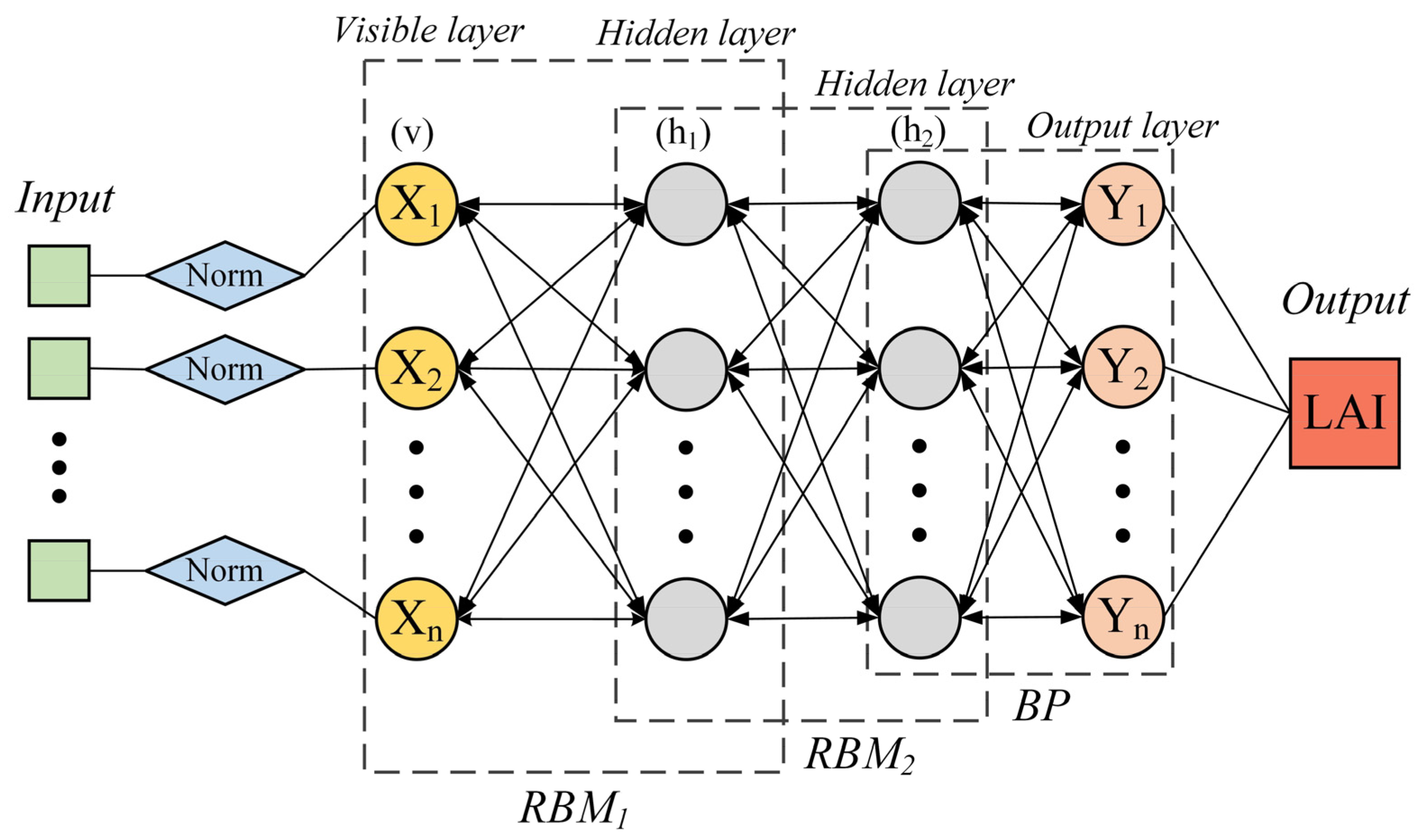
2.3.1. Deep Belief Network

Machine learning plays an important role in environmental remote sensing research. DL is a typical and advanced machine learning architecture with a strong ability of autonomous learning and fitting complex equations [61]. To date, the four mainstream DL architectures include the autoencoder (AE), the convolutional NN (CNN), the deep belief network (DBN), and the recurrent NN (RNN) [62]. DBN based on a restricted Boltzmann machine (RBM) [63] is a probability generation model (Figure 3). It is a typical artificial NN model that is composed of multiple RBMs stacked from bottom to top and constrained by the BP network. Compared with traditional NNs, the DBN overcomes the shortcomings of local optimization and a long training time caused by the random initialization of weighted parameters and can effectively solve the problems of gradient disappearance and explosion. Therefore, we selected the DBN to realize the training of the LAI inversion model in this paper.

The input data and output data of the DBN are the input layer and output layer of the network, respectively, and the input data are the parameters (reflectance of bands 1–7 and three angles) in the simulated LUT. Due to the large difference in the order of magnitude of these parameters, direct training will lead to an unbalanced expression of different information in the input data. Therefore, it needs to be normalized according to the unified rules, as shown in Equations (5) and (6). The output data include the LAI. The multiple RBMs in the middle are the hidden layers of the network that are bidirectionally fully connected via weights and biases. The calculation from remote sensing data to the LAI can be realized by weights and biases, that is, the inversion of the LAI.

$$X_i^{°}=\frac{X_i}{X_{i\_\max }},i=1,2,\dots ,10$$

(5)

$$Y^{°}=\frac{Y}{Y_{\max }},$$

(6)

where $X_i$ and $X_i^{°}$ represent the i-th input data before and after normalization, respectively; $Y$ and $Y^{°}$ represent the output data before and after normalization, respectively; and $X_{i\_\max }$ and $Y_{\max }$ represent the maximum value of the i-th input data and output data, respectively.

The training process of the DBN is primarily divided into two steps: using the generation model during the pre-training process and using the BP model during the fine-tuning stage [64]. The specific steps are as follows: (1) pre-training. Each layer of the RBM is trained independently and unsupervised to ensure that the feature information is preserved as much as possible when the eigenvector is mapped to the different feature spaces. (2) Fine-tuning. The last layer of the DBN is the BP network that receives the eigenvector output by the RBM and trains the entity relation classifier supervised. Therefore, the BP network propagates the error information to each layer and fine-tunes the weight of each layer to obtain the final DBN model. This idea is equivalent to seeking the local optimum first and then the global optimum. The network parameters can then be tuned by pre-training and optimization to obtain the best DBN LAI inversion model. This training method can not only speed up the training speed of the model but also easily obtain better initial parameter values after fine-tuning. This enables the DBN to overcome the shortcomings of easily falling into the local optimum and a long training time due to the random initialization of the weight parameters.

2.3.2. Training the DBN LAI Model

The construction of the DBN LAI inversion model primarily includes the design of the network structure and the initialization parameters. With sample data, the number of layers and neurons of the DBN are determined. In theory, the more layers and neurons, the higher the training accuracy will be. However, at the same time, this may lead to overfitting and reduce the accuracy. In this study, 80% of the sample dataset were randomly selected as training samples for training, and the remaining 20% for testing to verify the accuracy of the network training. Finally, it was determined that the number of hidden layers of the DBN LAI inversion model was two, and the number of neurons in each hidden layer was 10. Among the settings of the initialization parameters, the training batch and the training iterations are the two most important parameters that directly affect the efficiency and accuracy of model training. The training batch is the size of each block extracted from the sample dataset during the training process, which needs to be divisible by the total number of samples. The training batch can directly affect the training efficiency, the convergence speed, and the accuracy of the model. Hence, it is necessary to reasonably set these according to the test. Training iterations is the number of times the DBN network is trained. When it is too few, the data cannot be deeply mined and the model is prone to fall into a local optimum. When it is too many, the training time will be increased and the training efficiency will be reduced, while the model accuracy will no longer be improved. Therefore, it is necessary to test different values of parameters to determine the reasonable settings to ensure the training efficiency and accuracy of the DBN LAI inversion model. According to the experiment, it was finally determined that the training batch was 800 and the training iterations were 20,000. After the network construction and parameters settings were completed, the simulated TOA LUT was used to train the DBN and the weights and biases of the connections between the hidden layers could be obtained. The weights and biases were saved in the form of a network, and the network structure and related parameters were saved at the same time to obtain the LAI inversion model.

2.4. Error Metrics

The evaluation of inversion results is quantified by the following metrics: the Pearson correlation coefficient (r), the mean absolute error (MAE), and the root mean square error (RMSE). r is used to measure the correlation between two variables. MAE is the mean of the deviation between the model predicted value and the true value. RMSE is used to quantify the deviation between the predicted value and the true value. The specific calculation equations of these evaluation metrics are shown in Equations (7)–(9):

$$r=\frac{{\displaystyle \sum _{i=1}^n(x_i-\overline{x})(y_i-\overline{y})}}{\sqrt{{\displaystyle \sum _{i=1}^n{(x_i-\overline{x})}^2{\displaystyle \sum _{i=1}^n{(y_i-\overline{y})}^2}}}}$$

(7)

$$\mathrm{RMSE}=\sqrt{\frac{1}{n}{\displaystyle \sum _{i=1}^n{(x_i-y_i)}^2}}$$

(8)

$$\mathrm{MAE}=\frac{1}{n}{\displaystyle \sum _{i=1}^n\left|x_i-y_i\right|},$$

(9)

where $x_i$ and $y_i$ are the i-th LAI inversion result and ground-measured LAI, respectively; $\overline{x}$ and $\overline{y}$ are the averages of the LAI inversion result and ground-measured LAI, respectively; and $n$ is the number of ground-measured data points for validation.

3. Results and Validation

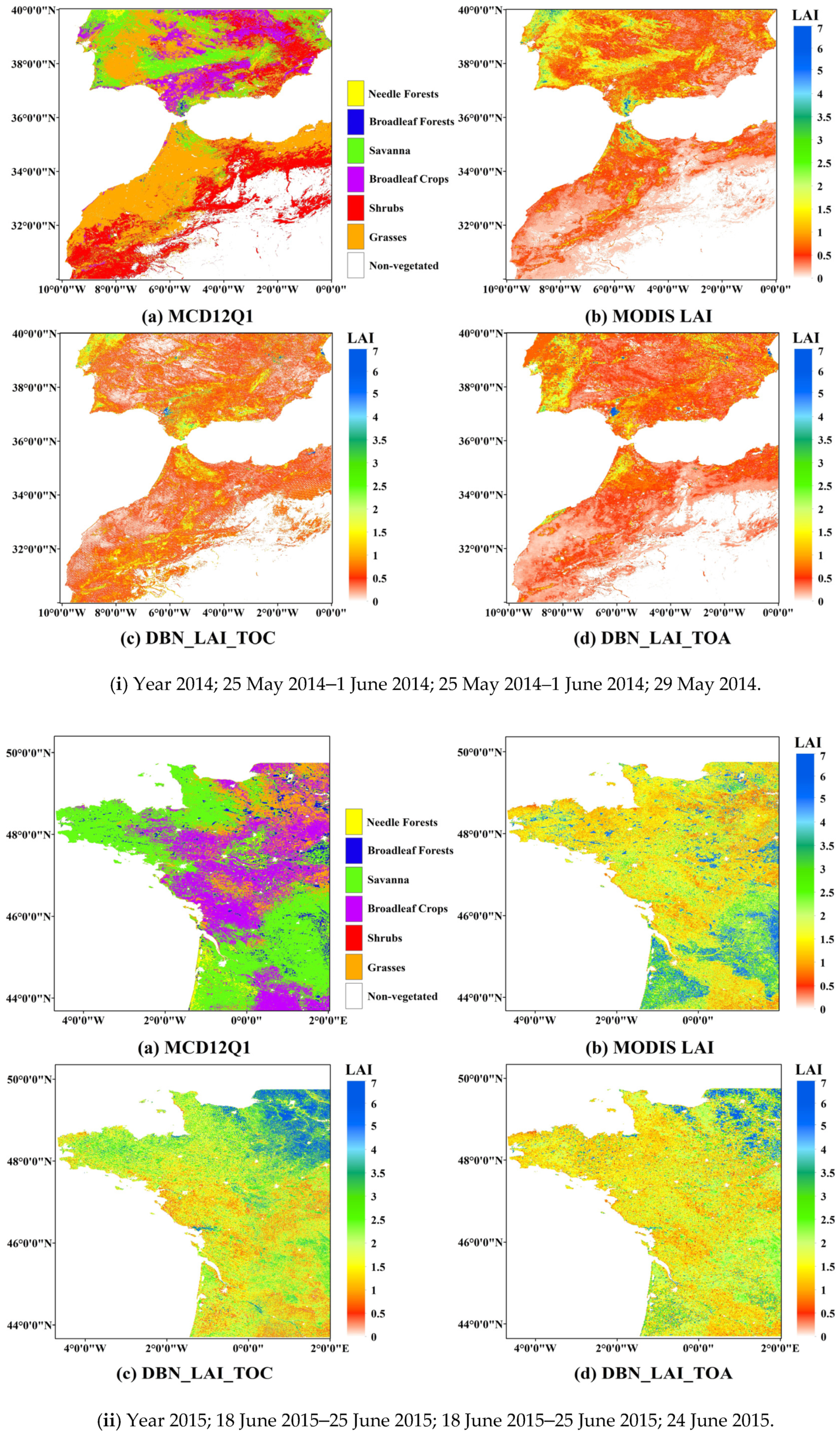
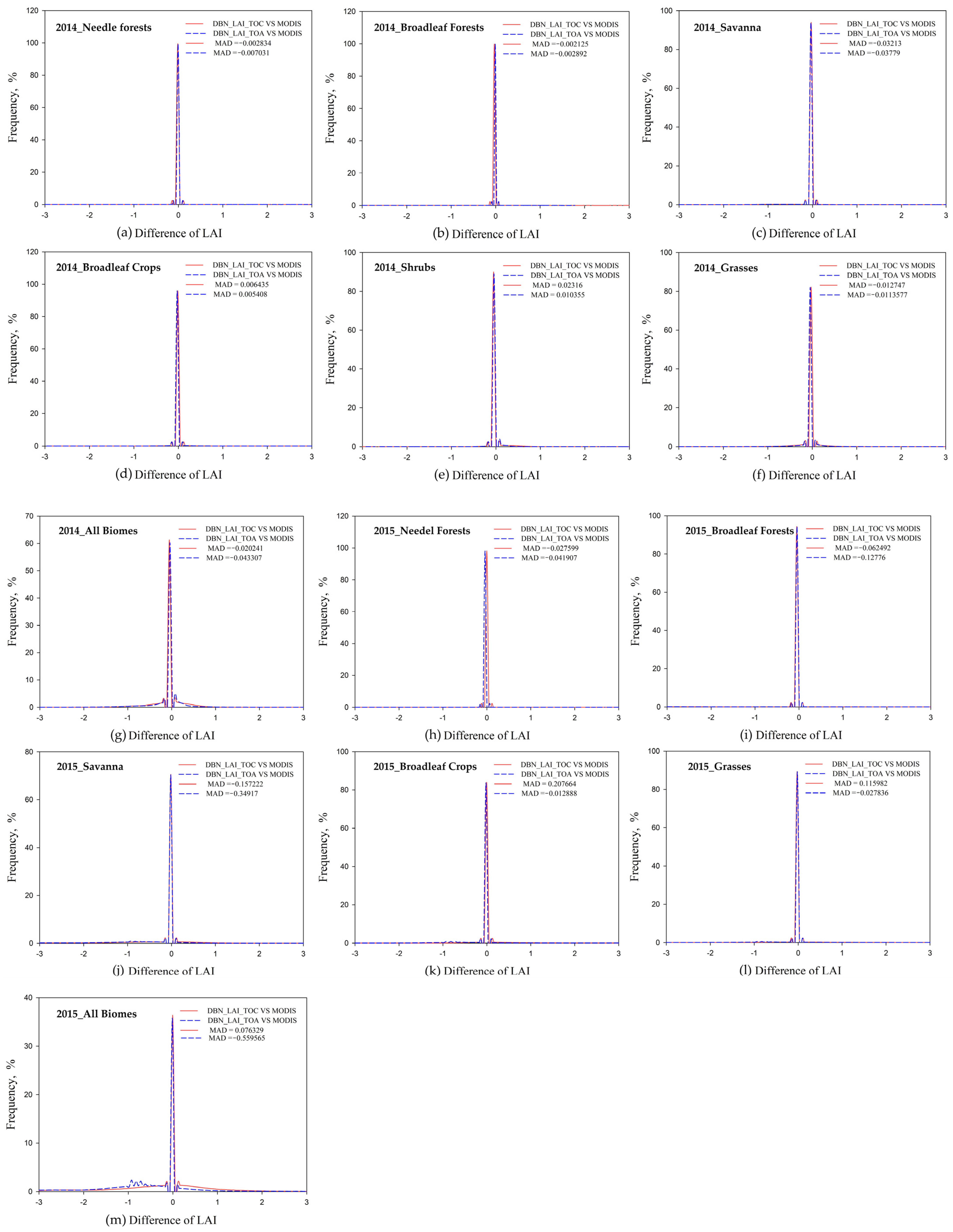
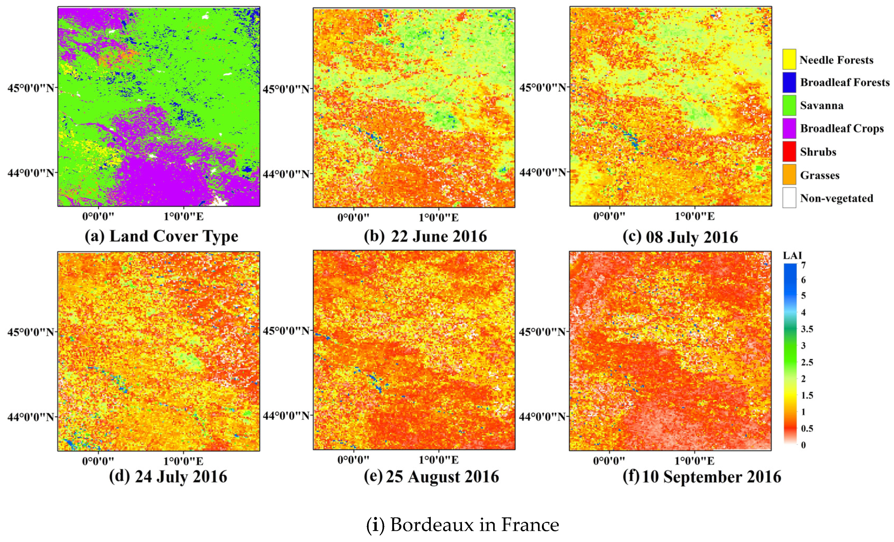
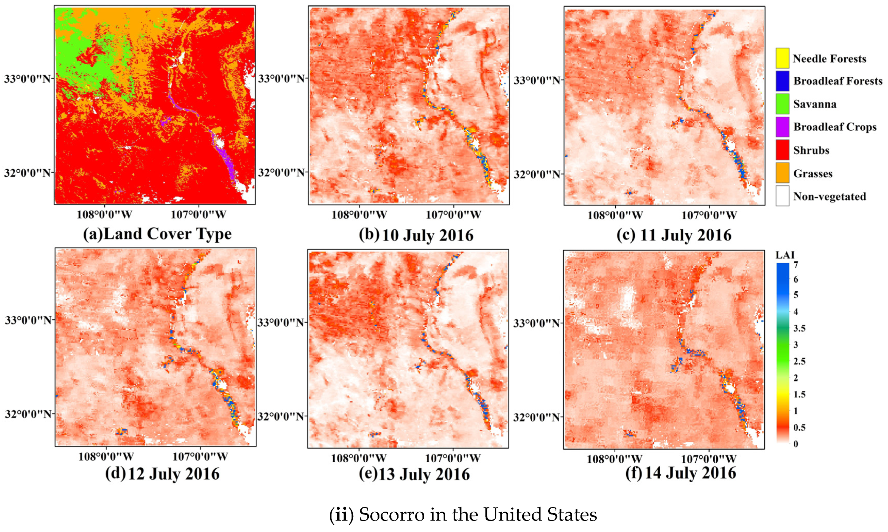
3.1. LAI Retrieval from TOC and TOA Reflectance

With the support of the data simulated by PROSAIL and the 6S model, the LAI inversion model was obtained by training the DBN. The DBN_LAI_TOC (LAI retrieved from MOD09A1) and the DBN_LAI_TOA (LAI retrieved from MOD021KM) were retrieved by inputting the reflectance of bands 1–7 and three angles into the LAI inversion model trained by the DBN. The TOC reflectance used in this study was the MODIS surface reflectance product (MOD09A1 data). The TOA reflectance data used in this study came from the MODIS L1B data (MOD021KM). We randomly selected two regions to demonstrate the LAI inversion results of our method. As shown in Figure 4, these two areas cover Spain and France, respectively. For the specific geographic location, please refer to the latitude and longitude information in Figure 4. Panel (a) MCD12Q1 is the land cover type, and panel (b) MODIS LAI is the MOD15A2H. Panels (c) and (d) are the DBN_LAI_TOC and the DBN_LAI_TOA (herein after collectively referred to as the DBN LAI), respectively, of the LAI inversion results at the TOC scale and TOA scale based on the DBN algorithm. Among them, the DBN_LAI_TOC has a spatial resolution of 500 m and a temporal resolution of eight days, and the DBN_LAI_TOA has a spatial resolution of 1 km and a temporal resolution of one day. The time information of these four panels has been indicated in Figure 4.

In order to intuitively express the difference between DBN LAI and MODIS LAI, we made an intercomparison between DBN_LAI_TOC, DBN_LAI_TOA and MODIS LAI, respectively, and plotted the LAI difference frequency distribution statistics for each year and for each of the six biomes (Figure 5). In order to unify the spatial resolution of different LAIs, we resampled MODIS LAI and DBN_LAI_TOC to 1km before calculating the LAI difference. Figure 5a–g and Figure 5h–m correspond to these two regions of Figure 4(i) and Figure 4(ii), respectively. Looking at all the difference frequency plots in Figure 5, it can be seen that the LAI difference varies around zero. Taking MODIS LAI as the reference, when the difference of LAI is less than zero, it means that the DBN algorithm underestimates LAI, and, when it is greater than zero, it means that the LAI is overestimated.

For the selected region in 2014, there was no obvious difference between DBN LAI and MODIS LAI for each year and for each of the six biomes. However, the slight difference can be seen in the calculated mean average difference (MAD) of LAI. On the land cover of needle forests, broadleaf forests, and savanna, the MAD of DBN_LAI_TOA was larger than that of DBN_LAI_TOC; on broadleaf crops, shrubs, and grasses, the MAD of DBN_LAI_TOA was smaller than that of DBN_LAI_TOC. On the land cover of needle forests, broadleaf forests, savanna, and grasses, the MAD of DBN_LAI_TOC and DBN_LAI_TOA were both less than zero, which means that, taking MODIS LAI as a reference, the frequency of underestimating LAI is higher. For broadleaf crops and shrubs, the MAD of both DBN LAI is greater than zero, which meant that the frequency of overestimating LAI is higher. From Figure 5g, we can see that, for all the biomes, DBN_LAI_TOC and DBN_LAI_TOA both underestimated LAI compared with MODIS LAI, and the underestimation frequency of DBN_LAI_TOA was higher than that of DBN_LAI_TOC. For the region in 2015, no matter for each biome or all the biomes, DBN_LAI_TOA had a higher frequency of underestimating LAI, while DBN_LAI_TOC had a higher frequency of underestimating LAI in needle forests, broadleaf forests, and savanna, but the frequency of LAI overestimation was high on broadleaf crops, grasses, and all the biomes. Furthermore, the MAD of DBN_LAI_TOA was smaller than that of DBN_LAI_TOC except on two land covers of broadleaf crops and grasses, while the MAD of DBN_LAI_TOA was greater than that of DBN_LAI_TOC on several other land covers and on all the biomes. This is consistent with the conclusion obtained from the difference statistical distribution histogram in 2014; that is, the difference between DBN_LAI_TOC and MODIS LAI is smaller than that of DBN_LAI_TOA.

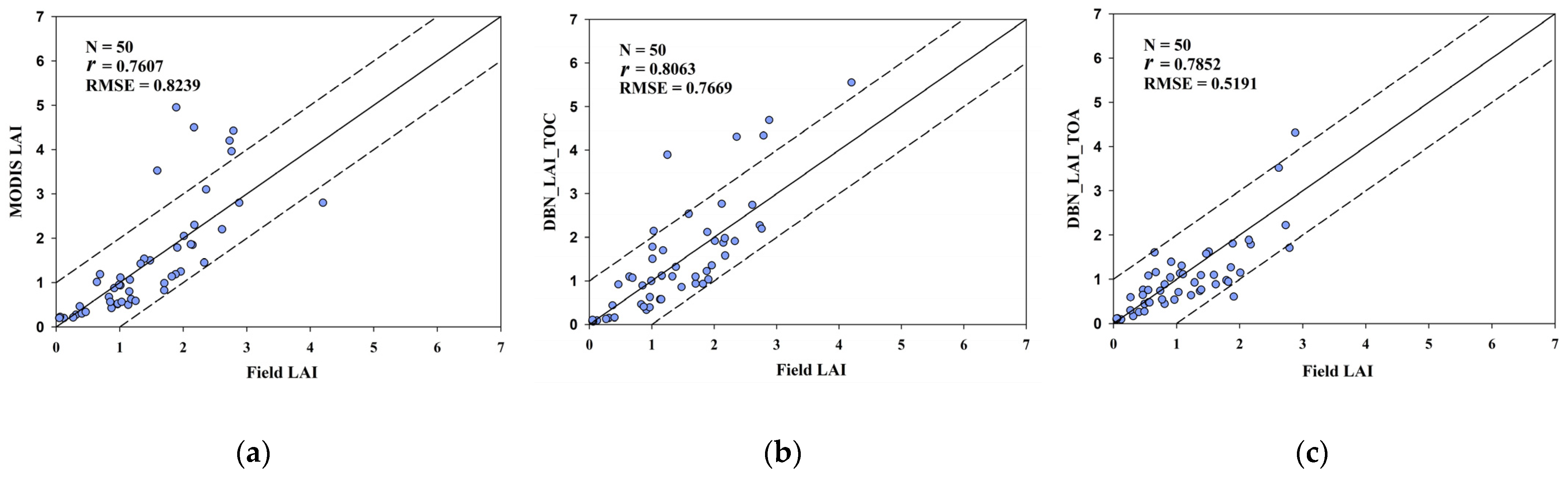
3.2. Validation against the DIRECT 2.0 Database

The performance of the DBN LAI inversion model was evaluated according to the ground dataset of DIRECT 2.0. When evaluating and verifying medium-resolution LAI products, ground “point” measurements are not suitable for direct comparison with medium-resolution pixels due to the influence of surface heterogeneity. Therefore, to reduce the influence of geometric registration on the verification, the mean 3 km × 3 km LAIs provided by DIRECT 2.0 were used for the direct verification. In spatial terms, MOD09A1 and MOD15A2H both have resolutions of 500 m. Therefore, we first resampled these images with a 500 m resolution to 1 km. We then selected 3 × 3 pixels around the center pixel (i.e., 3 km × 3 km) according to the site location and calculated the average value of these pixels to make the location correspond to the range of ground sites. Similarly, the resolution of MOD021KM is 1km, so we selected 3 × 3 pixels around the center pixel (i.e., 3 km × 3 km) and calculated the average value of these pixels to make the pixels spatially matched with the ground sites. In terms of time, the MODIS LAI and the DBN LAI that were the same or close to the ground measurement time were selected for verification. It means that, if the LAI is daily data, select the image with the same time as the ground LAI measurement; if the LAI is 8-daily data, select the image that contains the ground LAI measurement time in these 8 days. Figure 6 shows the comparison between the DIRECT 2.0 ground-measured LAI and the different LAI products, and the error statistics are shown in Table 3. The calculation equations of the quantitative evaluation error metrics are given in Section 2.4.

Figure 6a–c is the comparisons of the MODIS LAI, the DBN_LAI_TOC, the DBN_LAI_TOA, and the ground-measured LAI. The horizontal axis represents the ground-measured LAI, and the vertical axis represents the MODIS LAI, the DBN_LAI_TOC, and the DBN_LAI_TOA. These in situ data are available site data after cloud filtering. The validation results showed that, compared with the ground-measured LAI, the DBN_LAI_TOC (r = 0.8063) had a similar performance to the DBN_LAI_TOA (r = 0.7852), and both were greater than the MODIS LAI (r = 0.7607). Both the MODIS LAI and the DBN LAI had RMSE < 1.0, but the RMSE showed that the MODIS LAI was slightly inferior to the DBN LAI. The DBN_LAI_TOA had the smallest RMSE = 0.5191, followed by the DBN_LAI_TOC (RMSE = 0.7669), and both were smaller than the MODIS LAI (RMSE = 0.8239). The MAE can avoid the problem of the mutual cancellation of errors and can accurately reflect the size of the actual prediction error. The MAE of the MODIS LAI (MAE = 0.5311) and the DBN_LAI_TOC (MAE = 0.5527) was not significantly different, and both were greater than that of the DBN_LAI_TOA (MAE = 0.3865). In

Table 4. Error statistics of the verification results.

Error Statistics	N	r	RMSE	MAE
MODIS LAI	50	0.7607	0.8239	0.5311
DBN_LAI_TOC	50	0.8063	0.7669	0.5527
DBN_LAI_TOA	50	0.7852	0.5191	0.3865

, N represents the number of samples of the ground-measured LAI. The above demonstrates that the two LAI inversion models trained by the DBN algorithm had similar performances and high inversion accuracies.

4. Discussion

To simplify the process of drawing the vegetation LAI map from satellite data, an NN method that does not require complex atmospheric corrections was used in this paper to retrieve the LAI from the TOA reflectance. This method was applied to the MODIS sensor to test its effectiveness. The TOA-based retrieval method was expected to perform somewhat inferiorly due to the additional variability introduced into the LUT_B by means of the coupling with atmosphere simulations. However, its retrieval performance could not be considered worse than that of the TOC-based retrieval method. The r and the MAE of the TOC were better than the TOA, but the RMSE of the TOA was better than the TOC. This reveals that the LAI retrieval from the TOC and TOA reflectance data performs well on different evaluation metrics, respectively.

4.1. Performance of the TOA Retrieval

It can be seen from the LAI inversion results (Figure 4) that the spatial distribution of the DBN_LAI_TOC and the DBN_LAI_TOA was in good agreement with the MODIS LAI, and the distribution of the LAI was basically consistent with the vegetation region in the land cover type map (MCD12Q1). Different land cover types can be reflected to a certain extent according to the difference in the LAI values. Figure 4 shows that, for the surface type of the broadleaf crops (marked as purple in panel (a)), the two LAI inversion results of the DBN algorithm are better than the MODIS LAI. This may have been because the MODIS LAI retrieval algorithm underestimated the regions with higher LAIs. This possibility has been mentioned in the literature [65]. For the surface type of savanna (marked as green in panel (a)), the MODIS LAI was higher, while the LAI retrieved by the DBN algorithm was lower. The same conclusion can be obtained in the statistical distribution of LAI differences (Figure 5). We noticed that DBN_LAI_TOA obviously underestimated LAI in the selected area (year 2015). Referring to Figure 4(ii), we can find that this underestimation occurred in the land cover type of savanna. For the other land cover types, there was no significant difference between the MODIS LAI and the DBN LAI, which indicated that the DBN algorithm had a good performance for LAI retrieval. In addition, we can also see from Figure 5 that, compared with MODIS LAI, DBN LAI has both underestimation and overestimation. However, in general, the difference with MODIS LAI is mainly around zero, so we conclude that the method proposed in this paper is feasible.

Terra MODIS and Aqua MODIS view the entire Earth’s surface every 1–2 days, so their observation data have important indications in vegetation dynamic monitoring and land cover type changes. During the vegetation growth period, the vegetation LAI varies greatly in a short time, and the satellites with a low revisit time cannot acquire images every day. However, MODIS can acquire images daily and draw LAI maps under cloud-free conditions. Figure 7(i) shows the LAI inversion map of a selected area with fewer clouds in the west of Bordeaux, France. It can be seen from Figure 7(i) that the LAI of the vegetation in this area showed a trend from high to low in a period, which indicated a vegetation growth trend from vigorous to senescence. The days interval of the selected images is 16 or a multiple of 16. This is because the revisit period of MODIS was 16 days, and the subsatellite point positions of the satellites will coincide every 16 days; that is, the satellite observation geometry is repeated. This also shows that the changes in the LAI during this period were caused by vegetation growth dynamics rather than other factors, such as acquisition geometry variations. Figure 7(ii) shows the LAI inversion map of a cloud-free area in Socorro, Mexico for five consecutive days (10 July 2016–14 July 2016). As can be seen in Figure 7(ii), the LAI in this area has a slight variation during these five days, which may be caused by the difference in image acquisition geometry as the LAI of most biomes did not change significantly in a short time. Although MODIS can acquire images at a high frequency, the area and probability of images being covered by clouds is also very large, and it is difficult to find an area without clouds for many consecutive days. Therefore, we selected this area as a demonstration.

4.2. Advantages and Limitations of the Method Used

In this paper, the LUT simulated by the PROSAIL+6S RT model was utilized to obtain the LAI inversion model through DBN training without any prior information. The LAI retrieval method based on the TOA reflectance data omits the atmospheric correction process, simplifying the step of obtaining the LAI from satellite data. In addition, it provides an important contribution to the retrieval of LAI from sensors that do not provide atmospheric correction datasets. The DBN algorithm can fully mine the vegetation information carried in visible light and the NIR bands so as to effectively estimate the LAI based on spectral information. Although the method used in this paper had positive performance for the retrieval of the LAI, there are still limitations in this method as follows: (1) the MOD021KM and ground-measured LAI are single-day measurements, while the MOD09A1 and MOD15A2H data we used were eight-day synthetic data. This time difference had little influence on most vegetation types, but, for vegetation types such as farmland and grasslands, the LAI may fluctuate greatly in a short period, resulting in a certain difference in the LAI inversion results. (2) During the LAI verification, the area that was consistent with the same range as the ground sites (3 km × 3 km) was selected for spatial matching and then the average value was taken. This was then compared with the ground-measured LAI. Although spatial consistency was ensured, it will still inevitably cause errors due to the scale conversion. (3) Since the primary purpose of this paper was to verify the effectiveness of the algorithm, only the field data during the mid-latitude summer were selected for verification. However, for the mid-latitude summer data selected from the DIRECT 2.0 database, the land cover is mainly crops, and there are few sites with forest land cover, which leads to the maximum LAI value of the selected sites being only 2.88. Therefore, the effectiveness of our algorithm is unknown for land cover types with high LAI (>3). This verification method makes sense for land cover with low LAI (<3), but it would be incomplete for producing a global LAI product.

5. Conclusions

This study aimed to obtain a biophysical variable (LAI) of the vegetation canopy from the TOA reflectance using the NN method and apply it to the MODIS sensor to verify the effectiveness of this method. The LAI was successfully retrieved by inputting the spectral information in the visible and NIR bands (bands 1–7) and the observation geometry of MODIS into the model trained by the NN. To do so, the PROSAIL model was coupled with the 6S model to simulate a LUT about the TOA reflectance and associated input variables. Then, the LUT was trained by the DBN to construct an LAI inversion model. The LUT simulated in this study was applicable to all the biomes and considered different illumination-view geometrics.

We performed qualitative and quantitative evaluations on the MODIS LAI, the DBN_LAI_TOC, and the DBN_LAI_TOA. The qualitative evaluation was for a comparison of the spatial consistency of the different LAIs. It can be seen from Figure 4 that the MODIS LAI and the DBN LAI had good spatial consistency. The quantitative evaluation was for a comparison of the difference between the different LAIs and the MODIS LAI and the ground-measured LAI. We calculated the difference between DBN LAI and MODIS LAI and plotted the LAI difference frequency distribution histograms (Figure 5). From this figure, we can see that, for all the biomes, overall, the difference statistics in 2014 and 2015 show that the MAD of DBN_LAI_TOC (MAD = −0.020241 in 2014; MAD = 0.076329 in 2015) is smaller than that of DBN_LAI_TOA (MAD = −0.043307 in 2014; MAD = −0.559565 in 2015). In other words, the DBN LAI values retrieved from surface reflectance data are less different from the MODIS LAI, but this does not deny the feasibility of the LAI inversion method based on the TOA reflectance data. The DIRECT 2.0 ground database was used in this study to directly verify the DBN LAI inversion results and compare them with the MODIS LAI. According to the error metric r in Figure 6, we inferred that the correlation between the DBN LAI and the ground-measured LAI was very similar to the MODIS LAI. In addition, according to the RMSE, we conclude that, compared with the MODIS LAI, the deviation between the DBN LAI and the ground-measured LAI was smaller, indicating that the DBN LAI had better consistency with the ground-measured LAI. Moreover, from Table 4, we can see that the MAE of the DBN_LAI_TOC was similar to that of the MODIS, but both were greater than the DBN_LAI_TOA. This reflects that the actual prediction error of the LAI estimated from the TOA reflectance was the smallest. Therefore, the method proposed in this study performed well in LAI inversion.

In summary, the inversion and validation results showed that the LAI estimation could be achieved directly from the TOA reflectance. The LAI retrievals based on the TOC and the TOA reflectance data had similar performances. This indicated that the LAI retrieval could be achieved without atmospheric correction under clear sky conditions. The LAI retrieval based on the TOA reflectance can omit the step of atmospheric correction. For sensors that do not provide atmospheric correction datasets, retrieving the LAI from the TOA reflectance may be a better solution if atmospheric corrections are considered to introduce large uncertainties in the surface reflectance (TOC reflectance). This idea of using TOA reflectance data to retrieve biochemical parameters has a certain reference significance for other satellite data or for being used to retrieve other land surface parameters (e.g., FAPAR and FCOVER).

References

1. Xiao, Z.; Liang, S.; Wang, J.; Xiang, Y.; Zhao, X.; Song, J. Long-time-series global land surface satellite leaf area index product derived from MODIS and AVHRR surface reflectance. IEEE Trans. Geosci. Remote Sens. 2016, 54, 5301–5318. [Google Scholar] [CrossRef]
2. Xiao, Z.; Liang, S.; Sun, R.; Wang, J.; Jiang, B. Estimating the fraction of absorbed photosynthetically active radiation from the MODIS data based GLASS leaf area index product. Remote Sens. Environ. 2015, 171, 105–117. [Google Scholar] [CrossRef]
3. Bacour, C.; Baret, F.; Béal, D.; Weiss, M.; Pavageau, K. Neural network estimation of LAI, fAPAR, fCover and LAI×Cab, from top of canopy MERIS reflectance data: Principles and validation. Remote Sens. Environ. 2006, 105, 313–325. [Google Scholar] [CrossRef]
4. Chen, Z.; Yu, K.; Liu, J.; Wang, F.; Zhong, Y. Decreasing the error in the measurement of the ecosystem effective leaf area index of a Pinus massoniana forest. J. For. Res. 2018, 30, 1459–1470. [Google Scholar] [CrossRef]
5. Chen, J.M.; Black, T.A. Defining leaf area index for non-flat leaves. Plant Cell Environ. 1992, 15, 421–429. [Google Scholar] [CrossRef]
6. Myneni, R.B.; Hoffman, S.; Knyazikhin, Y.; Privette, J.L.; Glassy, J.; Tian, Y.; Wang, X.; Song, Y.; Zhang, G.R.; Smith, A.; et al. Running. Global products of vegetation leaf area and absorbed PAR from year one of MODIS data. Remote Sens. Environ. 2002, 83, 214–231. [Google Scholar] [CrossRef] [Green Version]
7. Ranga, B.; Myneni, J.R.; Asrar, G. A review on the theory of photon transport in leaf canopies. Agric. For. Meteorol. 1989, 45, 1–153. [Google Scholar] [CrossRef]
8. Arora, V. Modeling vegetation as a dynamic component in soil-vegetation-atmosphere transfer schemes and hydrological models. Rev. Geophys. 2002, 40, 3-1–3-26. [Google Scholar] [CrossRef] [Green Version]
9. GCOS. Systematic Observation Requirements for Satellite-Based Products for Climate. Available online: http://www.wmo.ch/web/gcos/gcoshome.html (accessed on 28 February 2022).
10. Yin, G.; Li, J.; Liu, Q.; Zhong, B.; Li, A. Improving LAI spatio-temporal continuity using a combination of MODIS and MERSI data. Remote Sens. Lett. 2016, 7, 771–780. [Google Scholar] [CrossRef]
11. Xu, B.; Park, T.; Yan, K.; Chen, C.; Zeng, Y.; Song, W.; Yin, G.; Li, J.; Liu, Q.; Knyazikhin, Y.; et al. Analysis of global LAI/FPAR products from VIIRS and MODIS Sensors for spatio-temporal consistency and uncertainty from 2012–2016. Forests 2018, 9, 73. [Google Scholar] [CrossRef] [Green Version]
12. Knyazikhin, Y.; Martonchik, J.V.; Diner, D.J.; Myneni, R.B.; Verstraete, M.; Pinty, B.; Gobron, N. Estimation of vegetation canopy leaf area index and fraction of absorbed photosynthetically active radiation from atmosphere-corrected MISR data. J. Geophys. Res. Atmos. 1998, 103, 32239–32256. [Google Scholar] [CrossRef] [Green Version]
13. Wenze, Y.; Bin, T.; Dong, H.; Rautiainen, M.; Shabanov, N.V.; Wang, Y.; Privette, J.L.; Huemmrich, K.F.; Fensholt, R.; Sandholt, I.; et al. MODIS leaf area index products: From validation to algorithm improvement. IEEE Trans. Geosci. Remote Sens. 2006, 44, 1885–1898. [Google Scholar] [CrossRef]
14. Baret, F.; Hagolle, O.; Geiger, B.; Bicheron, P.; Miras, B.; Huc, M.; Berthelot, B.; Niño, F.; Weiss, M.; Samain, O.; et al. LAI, fAPAR and fCover CYCLOPES global products derived from VEGETATION. Remote Sens. Environ. 2007, 110, 275–286. [Google Scholar] [CrossRef] [Green Version]
15. Fernandes, R.; Butson, C.; Leblanc, S.; Latifovic, R. Landsat-5 TM and Landsat-7 ETM+ based accuracy assessment of leaf area index products for Canada derived from SPOT-4 VEGETATION data. Can. J. Remote Sens. 2014, 29, 241–258. [Google Scholar] [CrossRef]
16. Claverie, M.; Matthews, J.; Vermote, E.; Justice, C. A 30+ Year AVHRR LAI and FAPAR climate data record: Algorithm description and validation. Remote Sens. 2016, 8, 263. [Google Scholar] [CrossRef] [Green Version]
17. Masson, V.; Champeaux, J.L.; Chauvin, F.; Meriguet, C.; Lacaze, R. A global database of land surface parameters at 1-km resolution in meteorological and climate models. J. Clim. 2003, 16, 1261–1282. [Google Scholar] [CrossRef]
18. Hu, J.; Su, Y.; Tan, B.; Huang, D.; Yang, W.; Schull, M.; Bull, M.A.; Martonchik, J.V.; Diner, D.J.; Knyazikhin, Y.; et al. Analysis of the MISR LAI/FPAR product for spatial and temporal coverage, accuracy and consistency. Remote Sens. Environ. 2007, 107, 334–347. [Google Scholar] [CrossRef] [Green Version]
19. Bicheron, P.; Leroy, M.; Hautecoeur, O. Retrieving of LAI and fAPAR with airborne POLDER data over various biomes. In Proceedings of the Geoscience & Remote Sensing, IGARSS 97 Remote Sensing—A Scientific Vision for Sustainable Development, Singapore, 3–8 August 1997; pp. 556–558. [Google Scholar]
20. Xiao, Z.; Liang, S.; Wang, J.; Chen, P.; Yin, X.; Zhang, L.; Song, J. Use of general regression neural networks for generating the GLASS leaf area index product from time-series MODIS surface reflectance. IEEE Trans. Geosci. Remote Sens. 2014, 52, 209–223. [Google Scholar] [CrossRef]
21. Xiang, Y.; Xiao, Z.Q.; Ling, S.L.; Wang, J.D.; Song, J.L. Validation of global land surface satellite (GLASS) leaf area index product. J. Remote Sens. 2014, 18, 57–596. [Google Scholar] [CrossRef]
22. Feng, D.; Chen, J.M.; Plummer, S.; Mingzhen, C.; Pisek, J. Algorithm for global leaf area index retrieval using satellite imagery. IEEE Trans. Geosci. Remote Sens. 2006, 44, 2219–2229. [Google Scholar] [CrossRef] [Green Version]
23. Copernicus Global Land Operations “Vegetation and Energy” “CGLOPS-1”. Available online: https://land.copernicus.eu/global/sites/cgls.vito.be/files/products/CGLOPS1_PUM_LC100m-V3_I3.4.pdf (accessed on 8 April 2022).
24. Fang, H.; Baret, F.; Plummer, S.; Schaepman-Strub, G. An overview of global leaf area index (LAI): Methods, products, validation, and applications. Rev. Geophys. 2019, 57, 739–799. [Google Scholar] [CrossRef]
25. Guo, H.; Liu, L.; Wang, C.; Lei, L.; Wu, Y.; Jiao, Q. Monitoring Chinese Spring Drought Using Time-Series MODIS data. In Proceedings of the Sixth International Symposium on Digital Earth: Data Processing and Applications, Beijing, China, 9–12 September 2009. [Google Scholar]
26. Raffy, M.; Soudani, K.; Trautmann, J. On the variability of the LAI of homogeneous covers with respect to the surface size and application. Int. J. Remote Sens. 2010, 24, 2017–2035. [Google Scholar] [CrossRef]
27. Ranga, B.; Myneni, R.R.N.; Steven, W. Running. Estimation of global leaf area index and absorbed par using radiative transfer models. IEEE Trans. Geosci. Remote Sens. 1997, 35, 1380–1393. [Google Scholar] [CrossRef] [Green Version]
28. Huete, A.R. A soil-adjusted vegetation index (SAVI). Remote Sens. Environ. 1988, 25, 295–309. [Google Scholar] [CrossRef]
29. Biudes, M.S.; Machado, N.G.; Danelichen, V.H.; Souza, M.C.; Vourlitis, G.L.; Nogueira, J.d.S. Ground and remote sensing-based measurements of leaf area index in a transitional forest and seasonal flooded forest in Brazil. Int. J. Biometeorol. 2014, 58, 1181–1193. [Google Scholar] [CrossRef]
30. Liu, Y.; Ju, W.; Chen, J.; Zhu, G.; Xing, B.; Zhu, J.; He, M. Spatial and temporal variations of forest LAI in China during 2000–2010. Chin. Sci. Bull. 2012, 57, 2846–2856. [Google Scholar] [CrossRef] [Green Version]
31. Liu, K.; Zhou, Q.-B.; Wu, W.-B.; Xia, T.; Tang, H.-J. Estimating the crop leaf area index using hyperspectral remote sensing. J. Integr. Agric. 2016, 15, 475–491. [Google Scholar] [CrossRef] [Green Version]
32. Duan, S.-B.; Li, Z.-L.; Wu, H.; Tang, B.-H.; Ma, L.; Zhao, E.; Li, C. Inversion of the PROSAIL model to estimate leaf area index of maize, potato, and sunflower fields from unmanned aerial vehicle hyperspectral data. Int. J. Appl. Earth Obs. Geoinf. 2014, 26, 12–20. [Google Scholar] [CrossRef]
33. Lek, S.; Guégan, J.F. Artificial neural networks as a tool in ecological modelling, an introduction. Ecol. Model. 1999, 120, 65–73. [Google Scholar] [CrossRef]
34. Yang, G.; Zhao, C.; Liu, Q.; Huang, W.; Wang, J. Inversion of a radiative transfer model for estimating forest LAI from multisource and multiangular optical remote sensing data. IEEE Trans. Geosci. Remote Sens. 2011, 49, 988–1000. [Google Scholar] [CrossRef]
35. Masemola, C.; Cho, M.A.; Ramoelo, A. Comparison of landsat 8 OLI and landsat 7 ETM+ for estimating grassland LAI using model inversion and spectral indices: Case study of Mpumalanga, South Africa. Int. J. Remote Sens. 2016, 37, 4401–4419. [Google Scholar] [CrossRef]
36. Smith, J.A. LAI inversion using a back-propagation neural network trained with a multiple scattering model. IEEE Trans. Geosci. Remote Sens. 1993, 31, 1102–1106. [Google Scholar] [CrossRef] [Green Version]
37. Hongliang, F.; Shunlin, L. Retrieving leaf area index with a neural network method: Simulation and validation. IEEE Trans. Geosci. Remote Sens. 2003, 41, 2052–2062. [Google Scholar] [CrossRef] [Green Version]
38. Estévez, J.; Berger, K.; Vicent, J.; Rivera-Caicedo, J.P.; Wocher, M.; Verrelst, J. Top-of-atmosphere retrieval of multiple crop traits using variational heteroscedastic gaussian processes within a hybrid workflow. Remote Sens. 2021, 13, 1589. [Google Scholar] [CrossRef]
39. Sun, L.; Wang, W.; Jia, C.; Liu, X. Leaf area index remote sensing based on Deep Belief Network supported by simulation data. Int. J. Remote Sens. 2021, 42, 7637–7661. [Google Scholar] [CrossRef]
40. MODIS Characterization Support Team (MCST). MODIS Level 1B Product User’s Guide For Level 1B Version 6.2.2 (Terra) and Version 6.2.1 (Aqua). 2017. Available online: https://mcst.gsfc.nasa.gov/sites/default/files/file_attachments/M1054E_PUG_2017_0901_V6.2.2_Terra_V6.2.1_Aqua.pdf (accessed on 8 March 2021).
41. MODIS Science Data Support Team. MODIS Level 1A Earth Location: Algorithm Theoretical Basis Document Version 3.0. 1997. Available online: https://modis.gsfc.nasa.gov/data/atbd/atbd_mod28_v3.pdf (accessed on 8 March 2021).
42. Garrigues, S.; Lacaze, R.; Baret, F.; Morisette, J.T.; Weiss, M.; Nickeson, J.E.; Fernandes, R.; Plummer, S.; Shabanov, N.V.; Myneni, R.B.; et al. Validation and intercomparison of global Leaf Area Index products derived from remote sensing data. J. Geophys. Res. Biogeosci. 2008, 113, G02028. [Google Scholar] [CrossRef]
43. Wei, H.; Cui, S.; Yang, S.; Zhao, Q. Sea surface temperature retrieving using MODIS data. J. Atmos. Environ. Opt. 2018, 13, 8. Available online: http://gk.hfcas.ac.cn/CN/Y2018/V13/I4/277 (accessed on 8 March 2021).
44. MODIS Characterization Support Team (MCST). MODIS 1 km Calibrated Radiances Product; NASA MODIS Adaptive Processing System, Goddard Space Flight Center: Greenbelt, MD, USA, 2017. [CrossRef]
45. MODIS Characterization Support Team (MCST). MODIS Geolocation Fields Product; NASA MODIS Adaptive Processing System, Goddard Space Flight Center: Greenbelt, MD, USA, 2017. [CrossRef]
46. NASA. MOD09A1 MODIS/Terra Surface Reflectance 8-Day L3 Global 500 m SIN Grid; NASA LP DAAC; NASA: Washington, DC, USA, 2017. [CrossRef]
47. Friedl, M.; Sulla-Menashe, D. MCD12Q1 MODIS/Terra + Aqua Land Cover Type Yearly L3 Global 500 m SIN Grid; NASA LP DAAC; NASA: Washington, DC, USA, 2015. [CrossRef]
48. Myneni, R.; Knyazikhin, Y.; Park, T.; MODAPS SIPS NASA. MYD15A2H MODIS/Aqua Leaf Area Index/FPAR 8-Day L4 Global 500 m SIN Grid; NASA LP DAAC; NASA: Washington, DC, USA, 2017. [CrossRef]
49. Friedl, M.A.; Sulla-Menashe, D.; Tan, B.; Schneider, A.; Ramankutty, N.; Sibley, A.; Huang, X. MODIS Collection 5 global land cover: Algorithm refinements and characterization of new datasets. Remote Sens. Environ. 2010, 114, 168–182. [Google Scholar] [CrossRef]
50. Knyazikhin, Y.; Glassy, J.; Privette, J.L.; Tian, Y.; Lotsch, A.; Zhang, Y.; Wang, Y.; Morisette, J.T.; Votava, P.; Myneni, R.B.; et al. MODIS Leaf Area Index (LAI) and Fraction of Photosynthetically Active Radiation Absorbed by Vegetation (FPAR) Product (MOD15). Algorithm Theoretical Basis Document Version 4.0. Available online: https://modis.gsfc.nasa.gov/data/atbd/atbd_mod15.pdf (accessed on 31 May 2019).
51. Knyazikhin, Y.; Martonchik, J.V.; Myneni, R.B.; Diner, D.J.; Running, S.W. Synergistic algorithm for estimating vegetation canopy leaf area index and fraction of absorbed photosynthetically active radiation from MODIS and MISR data. J. Geophys. Res. Atmos. 1998, 103, 32257–32275. [Google Scholar] [CrossRef] [Green Version]
52. Jacquemoud, S.; Verhoef, W.; Baret, F.; Bacour, C.; Zarco-Tejada, P.J.; Asner, G.P.; François, C.; Ustin, S.L. PROSPECT + SAIL models: A review of use for vegetation characterization. Remote Sens. Environ. 2009, 113, S56–S66. [Google Scholar] [CrossRef]
53. Hosgood, B.; Jacquemoud, S.; Andreoli, J.; Verdebout, A.; Pedrini, A.; Schmuck, G. Leaf Optical Properties Experiment 93 (LOPEX93); European Commission: Brussels, Belgium, 1995. [Google Scholar]
54. Wocher, M.; Berger, K.; Danner, M.; Mauser, W.; Hank, T. Physically-based retrieval of canopy equivalent water thickness using hyperspectral data. Remote Sens. 2018, 10, 1924. [Google Scholar] [CrossRef] [Green Version]
55. Tanré, D.; Deroo, C.; Duhaut, P.; Herman, M.; Morcrette, J.J.; Perbos, J.; Deschamps, P.Y. Technical note description of a computer code to simulate the satellite signal in the solar spectrum: The 5S code. Int. J. Remote Sens. 2010, 11, 659–668. [Google Scholar] [CrossRef]
56. Vermote, E.F.; Kotchenova, S. Atmospheric correction for the monitoring of land surfaces. J. Geophys. Res. 2008, 113. [Google Scholar] [CrossRef]
57. Vermote, E.F.; Tanré, D.; Deuze, J.L.; Herman, M.; Morcette, J.J. Second simulation of the satellite signal in the solar spectrum, 6S: An overview. IEEE Trans. Geosci. Remote Sens. 1997, 35, 675–686. [Google Scholar] [CrossRef] [Green Version]
58. Vermote, E.F.T.D.; Tanré, D.; Deuzé, J.L.; Herman, M.; Morcrette, J.J.; Kotchenova, S.Y. Second Simulation of a Satellite Signal in the Solar Spectrum-Vector (6SV). Available online: https://salsa.umd.edu/files/6S/6S_Manual_Part_1.pdf (accessed on 8 March 2021).
59. Vermote, E.F.; El Saleous, N.Z.; Justice, C.O. Atmospheric correction of MODIS data in the visible to middle infrared First results. Remote Sens. Environ. 2002, 83, 97–111. [Google Scholar] [CrossRef]
60. Vermote, E.F.; El Saleous, N.; Justice, C.O.; Kaufman, Y.J.; Privette, J.L.; Remer, L.; Roger, J.C.; Tanré, D. Atmospheric correction of visible to middle-infrared EOS-MODIS data over land surfaces: Background, operational algorithm and validation. J. Geophys. Res. Atmos. 1997, 102, 17131–17141. [Google Scholar] [CrossRef] [Green Version]
61. Wu, P.; Yin, Z.; Yang, H.; Wu, Y.; Ma, X. Reconstructing geostationary satellite land surface temperature imagery based on a multiscale feature connected convolutional neural network. Remote Sens. 2019, 11, 300. [Google Scholar] [CrossRef] [Green Version]
62. Yuan, Q.; Shen, H.; Li, T.; Li, Z.; Li, S.; Jiang, Y.; Xu, H.; Tan, W.; Yang, Q.; Wang, J.; et al. Deep learning in environmental remote sensing: Achievements and challenges. Remote Sens. Environ. 2020, 241, 111716. [Google Scholar] [CrossRef]
63. Geoffrey, E.; Hinton, S.O.; Yee-Whye, T. A fast learning algorithm for deep belief nets. Neural Comput. 2006, 18, 1527–1554. [Google Scholar] [CrossRef]
64. Larochelle, H.; Erhan, D.; Courville, A.; Bergstra, J.; Bengio, Y. An Empirical Evaluation of Deep Architectures on Problems with Many Factors of Variation. In Proceedings of the 24th International Conference on Machine Learning, Corvallis, OR, USA, 20–24 June 2007; Association for Computing Machinery: New York, NY, USA, 2007; pp. 473–480. [Google Scholar]
65. De Kauwe, M.G.; Disney, M.I.; Quaife, T.; Lewis, P.; Williams, M. An assessment of the MODIS collection 5 leaf area index product for a region of mixed coniferous forest. Remote Sens. Environ. 2011, 115, 767–780. [Google Scholar] [CrossRef]
Figure 1. Flow chart of the LAI retrieval based on PROSAIL and the 6S coupling model. Among these, the portion with the green background represents the process of simulating the TOC reflectance LUT with the PROSAIL model, and the portion with blue background represents the process of simulating the TOA reflectance LUT with the 6S model on this basis. Model A is an LAI inversion model suitable for the TOC reflectance, and model B is suitable for the TOA reflectance.
Remotesensing 14 02456 g001
Figure 2. Spatial distribution of the ground-measured LAI.
Remotesensing 14 02456 g002
Figure 3. DBN structure, where “norm” represents the normalization of the input data, and “v” and “h” represent the visible layer and hidden layer of each RBM layer, respectively.
Remotesensing 14 02456 g003
Figure 4. LAI inversion results. The four maps in each figure cover the same area. From (a) to (d), they represent the land cover type (MCD12Q1), the MODIS LAI (MOD15A2H), the DBN_LAI_TOC (LAI retrieval from the TOC reflectance using the DBN algorithm), and the DBN_LAI_TOA (LAI retrieval from the TOA reflectance using the DBN algorithm), respectively. The land cover type map only shows the vegetation coverage area, and the non-vegetation area is shown in white in panel (a).
Remotesensing 14 02456 g004
Figure 5. Statistics of LAI difference distribution between MODIS LAI and DBN LAI. The horizontal axis represents the difference of LAI, and the vertical axis represents the frequency (expressed as a percentage) of the difference distribution. The red solid line represents the difference between DBN_LAI_TOC and MODIS LAI, and the blue dashed line represents the difference between DBN_LAI_TOA and MODIS LAI. The “MAD” represents mean average difference of LAI. Panels (ag) correspond to the LAI differences of the six biomes in Figure 4(i), which are needle forests, broadleaf forests, savanna, broadleaf crops, shrubs, grasses, and all biomes in turn. Similarly, panels (hm) correspond to the LAI differences of different biomes in Figure 4(ii). It should be noted that there is no shrubs land cover in Figure 4(ii), so the LAI difference map for shrubs is missing.
Remotesensing 14 02456 g005
Figure 6. Scatterplot between the field-measured data and the (a) MODIS LAI, (b) DBN_LAI_TOC, and (c) DBN_LAI_TOA. The black solid line is the 1:1 line, and the red solid line is the regression line. The two intercepts of the dashed lines are ± 1 .
Remotesensing 14 02456 g006
Figure 7. LAI dynamic change maps. Panel (a) represents the land cover type, panels (bf) represent the LAI maps of the different Julian days.
Remotesensing 14 02456 g007aRemotesensing 14 02456 g007b