Regional Ionospheric Corrections for High Accuracy GNSS Positioning

Abstract

Centimetre-level accurate ionospheric corrections are required for a high accuracy and rapid convergence of Precise Point Positioning (PPP) GNSS positioning solutions. This research aims to evaluate the accuracy of a local/regional ionospheric delay model using a linear interpolation method across Australia. The accuracy of the ionospheric corrections is assessed as a function of both different latitudinal regions and the number and spatial density of GNSS Continuously Operating Reference Stations (CORSs). Our research shows that, for a local region of 5° latitude ×10° longitude in mid-latitude regions of Australia (~30° to 40°S) with approximately 15 CORS stations, ionospheric corrections with an accuracy of 5 cm can be obtained. In Victoria and New South Wales, where dense CORS networks exist (nominal spacing of ~100 km), the average ionospheric corrections accuracy can reach 2 cm. For sparse networks (nominal spacing of >200 km) at lower latitudes, the average accuracy of the ionospheric corrections is within the range of 8 to 15 cm; significant variations in the ionospheric errors of some specific satellite observations during certain periods were also found. In some regions such as Central Australia, where there are a limited number of CORSs, this model was impossible to use. On average, centimetre-level accurate ionospheric corrections can be achieved if there are sufficiently dense (i.e., nominal spacing of approximately 200 km) GNSS CORS networks in the region of interest. Based on the current availability of GNSS stations across Australia, we propose a set of 15 regions of different ionospheric delay accuracies with extents of 5° latitude ×10° longitude covering continental Australia.

1. Introduction

Applications of the Global Navigation Satellite Systems (GNSS) Precise Point Positioning (PPP) technique are rapidly increasing due to the methods computational efficiency, low communications bandwidth requirement and relative accuracy. PPP users can obtain position solutions with centimetre- to decimetre-level accuracy in static and kinematic modes [1,2,3]. The main advantage of PPP compared to differential based GNSS positioning techniques (e.g., Real Time Kinematics, RTK) is that PPP is based on the State-Space Representation (SSR) of corrections approach [4,5]. The SSR approach allows for GNSS-PPP-related errors such as satellite orbits and clocks to be modelled using a global sparse network of GNSS Continuously Operating Reference Stations (CORS) infrastructure. This removes the need for users to operate nearby base stations (i.e., base line < 100 km) or within a local GNSS CORS network. However, a drawback of PPP is its relatively long solution convergence time, which limits its adoption in real-time applications requiring almost instantaneous centimetre-level positioning accuracy [4]. Tens of minutes to a few hours is required for PPP solutions to provide coverage to centimetre-level accuracy [6,7]. A significant amount of research effort has been invested in the past decade to reduce the solution convergence time [8,9]. One known solution is to strengthen the PPP underlining measurement model by including externally computed, accurate ionospheric delay estimates into the end-user PPP algorithms [10,11,12,13,14].

For single-frequency PPP, ionospheric models such as the Klobuchar and the Global Ionospheric Maps (GIMs) estimated from a sparse global CORS network are applied. The accuracy of the ionospheric corrections derived from these models is approximately 15–20 TECu and 2–4 TECu, respectively [15], where one Total Electron Content unit (1 TECu) = 16 cm of ionospheric correction on L1 frequency. While these ionospheric correction models are useful in aiding precise single-frequency positioning, ionospheric corrections at 2–4 TECu are not sufficiently accurate to accelerate PPP convergence times from a few hours to minutes. PPP that uses two or more frequencies eliminates the need for an ionospheric model, as dual-frequency GNSS receivers can remove the first order (~99%) ionospheric delays by forming the ionosphere-linear combination. However, this linear combination of two signals, whilst removing the effects of the ionospheric delays, increases the noise amplification factor by three. This weakens the measurement model in dual-frequency PPP and results in a long solution convergence time of typically a couple of hours [12,16].

To facilitate a fast solution convergence time of a few minutes for PPP, the ionospheric corrections need to be accurate to less than one decimetre, that is, <~0.6 TECu. This requires the use of high-density local/regional CORS infrastructure networks to accurately estimate the ionosphere delay corrections, as in the case of network-based RTK. Hence, the terminology of “PPP-RTK” being a hybrid between the global PPP solutions and high-density local-network-based RTK solutions. The convergence time of a PPP-RTK solution depends on the accuracy of the ionosphere corrections (typically < 10 cm), which is dependent on the combination of the density of the local CORS networks and its latitudinal extent [17].

Geoscience Australia, through its Positioning Australia program, aims to accelerate the adoption and development of GNSS positioning technology and applications in Australia. The aim will be achieved by integrating and upgrading the country’s GNSS space-based infrastructure via the deployment of a Satellite-based Augmentation System (SBAS), and ground-based CORS infrastructure networks to provide high accuracy, high reliability fit-for-purpose GNSS positioning services throughout its territory [18]. The Analysis Centre Software (ACS), called ‘Ginan’, is a GNSS processing toolkit developed by Geoscience Australia for processing GNSS observations for geodetic applications, as well as computations of GNSS corrections products to enable high-accuracy GNSS applications. Ginan is a free-to-use open source and is made up of two distinct software entities: The Precise Orbit Determination (POD) and the Parameter Estimation Algorithm (PEA). PEA uses a Kalman filter to estimate precise satellite orbits from a global CORS network, as well as satellite clocks, vertical TEC and zenith troposphere delays. A country like Australia presents challenges when designing and developing a high-accuracy national GNSS positioning service. Australia is a vast landmass, most of which is sparsely populated and cannot economically justify hosting a high-density CORS network. Furthermore, Australia extends from 10° to almost 44° south, providing ionospheric disturbances at different scales.

This research assesses the achievable accuracy of a local ionospheric delay model for Australia based on the linear interpolation method. The assessment will be conducted by taking into consideration the number and spatial density of the GNSS CORS networks. The model is populated with points where the ionospheric effects are known—because these have been calculated based on readings taken at CORS. The effect of the ionosphere at a given point is calculated using a linear interpolation to that point from the known (CORS) points. As Australia has a large and sparsely populated landmass (its population and infrastructure are mainly concentrated along the coast), the density of the GNSS CORS networks across the continent is not uniformly distributed. Thus, it is also of interest to identify the optimum number of GNSS CORS stations, and the corresponding spatial density required to achieve centimetre-level ionospheric corrections, thus realising the ambition of the Australian Government Positioning program. The goal of this research is to contribute towards our understanding of the regions in Australia that may require the additional investment and densification of CORS infrastructure for enabling high-accuracy positioning. The accuracy of the derived ionospheric corrections will be evaluated as functions of different latitudinal regions and the spatial density of the GNSS CORS networks across Australia. The Ginan toolkit will be used to generate between-satellite single-difference ionosphere delay estimates. These estimates will then be used to derive a series of regional ionospheric grid maps that are 5° latitude × ~10° longitude in size.

2. Methodology

2.1. Ionosphere Delay Estimation Using PPP Technique

PPP calls for the explicit modelling and estimation of biases on the GNSS measurements. For this purpose, the undifferenced uncombined PPP measurement model is characterised as follows [19]:

$$L_{r,f}^s=R_r^s+c\left(d{t}_r-d{t}^s\right)+{\tau }_r^s-\frac{{\lambda }_f^2}{{\lambda }_1^2}{I}_r^s+\left(b_{r,f}+{\lambda }_f{N}_{r,f}^s-b_f^s\right)+\epsilon { }_{L,f}^s$$

(1)

$$P_{r,f}^s=R_r^s+c\left(d{t}_r-d{t}^s\right)+{\tau }_r^s+\frac{{\lambda }_f^2}{{\lambda }_1^2}{I}_r^s+B_{r,f}-B_f^s+{\epsilon }_{P,f}^s$$

(2)

where $L_{r,f}^s$ and $P_{r,f}^s$ are the carrier phase and pseudorange measurements corresponding to satellite s, station r and frequency f; $R_{r }^s$ is the geometric distance; $c$ is the speed of light; $d{t}_r$ and $d{t}^s$ are the receiver and satellite clock errors, respectively; ${\tau }_r^s$ is the slant troposphere delay between satellite and receiver; $I_r^s$ is the ionosphere delay along the line-of-sight from a satellite to a receiver; $N_{r,f}^s$ is the carrier phase ambiguity; ${\lambda }_f$ is the wavelength for the frequency f; $b_{r,f}$ and $B_{r,f}$ are the satellite hardware delays of the carrier phase and pseudorange measurements, respectively; $b_f^s$ and $B_f^s$ are the satellite hardware delays of the carrier phase and pseudorange measurements, respectively; $\epsilon { }_{L,f}^s$ and ${\epsilon }_{P,f}^s$ are the carrier phase and pseudorange measurement noises, respectively.

It is worth noting that the effects of the antenna phase centre offset and phase centre variation, solid earth tides, phase windup and relativistic effects have been corrected in the measurements. The Ginan toolkit is now capable of generating rapid and ultra-rapid orbit parameters, but, for the purposes of this research, the International GNSS Service (IGS) final products were used to correct for the satellite orbital errors.

The ionosphere-free combination of pseudoranges $\left(P_{r,IF}^s\right)$ and carrier phase measurements ($L_{r,IF }^s$) is taken as:

$$P_{r,IF}^s=\frac{{\lambda }_2^2}{{\lambda }_2^2-{\lambda }_1^2}{P}_{r,1}^s-\frac{{\lambda }_1^2}{{\lambda }_2^2-{\lambda }_1^2}{P}_{r,2}^s$$

(3)

$$L_{r,IF}^s=\frac{{\lambda }_2^2}{{\lambda }_2^2-{\lambda }_1^2}{L}_{r,1}^s-\frac{{\lambda }_1^2}{{\lambda }_2^2-{\lambda }_1^2}{L}_{r,2}^s$$

(4)

and replacing the satellite and receiver clock with:

$$d{t}_{IF,r}=d{t}_r+\frac{{\lambda }_2^2}{{\lambda }_2^2-{\lambda }_1^2}{B}_{r,1}-\frac{{\lambda }_1^2}{{\lambda }_2^2-{\lambda }_1^2}{B}_{r,2}$$

(5)

$$d{t}_{IF}^s=d{t}^s+\frac{{\lambda }_2^2}{{\lambda }_2^2-{\lambda }_1^2}{B}_1^s-\frac{{\lambda }_1^2}{{\lambda }_2^2-{\lambda }_1^2}{B}_2^s$$

(6)

Therefore, the $\left(L_{r,IF }^s\right)$ and $\left(P_{r,IF}^s\right)$ can be written as follows:

$$L_{r,IF}^s=R_r^s+c\left(d{t}_{IF, r}-d{t}_{IF}^s\right)+{\tau }_r^s+A_{r,IF}^s$$

(7)

$$P_{r,IF}^s=R_r^s+c\left(d{t}_{IF,r}-d{t}_{IF}^s\right)+{\tau }_r^s$$

(8)

Equations (7) and (8) can be used to estimate the station positions, the satellite clock offset $cd{t}_{IF}^s=cd{t}^s+B_{IF}^s$, station clock offset $cd{t}_{IF,r}=cd{t}_r+B_{r,IF}$ and the tropospheric delays ${\tau }_r^s$, as well as the real valued ambiguity $A_{r,IF}^s$ consisting of ambiguity plus the satellite and receiver hardware biases as shown in (9).

$$A_{r,IF}^s=b_{r,IF}-B_{r,IF}-b_{IF}^s+B_{IF}^s+\frac{{\lambda }_1{\lambda }_2}{{\lambda }_1+{\lambda }_2}{N}_{r,1}^s+\frac{{\lambda }_2{\lambda }_1^2}{{\lambda }_2^2-{\lambda }_1^2}\left(N_{r,1}^s-N_{r,2}^s\right)$$

(9)

The use of a wide-lane combination for ambiguity resolution is helpful due to their longer wavelength. Here, the Melbourne–Wübbena combination [20,21,22]

$$A_{r,MW}^s=\frac{{L^{\prime }}_{r,1}^s}{{\lambda }_1}-\frac{{L^{\prime }}_{r,2}^s}{{\lambda }_2}+\frac{{\lambda }_1-{\lambda }_2}{{\lambda }_1+{\lambda }_2}\left(\frac{{P^{\prime }}_{r,1}^s}{{\lambda }_1}+\frac{{P^{\prime }}_{r,2}^s}{{\lambda }_2}\right)$$

(10)

is used to isolate and resolve the wide-lane ambiguities $N_{r,WL}^s=N_{r,1}^s-N_{r,2}^s$. Equation (10) can be rewritten as

$$A_{r,MW}^s={\beta }_{r,MW}-{\beta }_{MW}^s+N_{r,WL}^s$$

(11)

where ${\beta }_{r,MW}$ and ${\beta }_{MW}^s$ are Melbourne–Wübbena combination receiver and satellite biases.

Once the wide-lane ambiguities have been solved, the ambiguity on the GPS L1 carrier phase can be isolated and resolved as well, as shown in (12).

$$\frac{{\lambda }_1+{\lambda }_2}{{\lambda }_1{\lambda }_2}{A}_{r,IF}^s+\frac{{\lambda }_1}{{\lambda }_1-{\lambda }_2}{N^{\prime }}_{r,WL}^s={\beta }_{r,IF}-{\beta }_{IF}^s+\frac{{\lambda }_1{\lambda }_2}{{\lambda }_1+{\lambda }_2}{N^{\prime }}_{r,1}^s$$

(12)

For enabling global PPP solutions, the satellite positions or orbits, the satellite clock offset $d{t}_{IF}^s$ and the phase bias estimates for GPS L1 and GPS L2 (${b^{\prime }}_1^s$, ${b^{\prime }}_2^s$) can be used to deliver ambiguity-resolved PPP solutions to the end user.

$${b^{\prime }}_1^s={\lambda }_1{\beta }_{IF}^s-\frac{{\lambda }_1^2}{{\lambda }_2-{\lambda }_1}{\beta }_{MW}^s$$

(13)

$${b^{\prime }}_2^s={\lambda }_2{\beta }_{IF}^s-\frac{{\lambda }_2^2}{{\lambda }_2-{\lambda }_1}{\beta }_{MW}^s$$

(14)

To obtain the ionosphere delay estimates used in this research, the carrier phase measurements for L1 and L2 were corrected using (15) and (16).

$${L^{″}}_{r,1}^s={L^{\prime }}_{r,1}^s-\left({b^{\prime }}_{r,1}+{\lambda }_1{N}_{r,1}^s-b_1^s\right)$$

(15)

$${L^{″}}_{r,2}^s={L^{\prime }}_{r,2}^s-\left({b^{\prime }}_{r,2}+{\lambda }_2{N^{\prime }}_{r,1}^s-{\lambda }_2{N}_{r,WL}^s-{b^{\prime }}_2^s\right)$$

(16)

The phase biases can be precisely estimated with the use of a global CORS network, and there are no errors associated with ambiguities once they are solved. Thus, the noise level of the corrected measurements is expected to be dominated by the un-modelled errors in the carrier phase measurement.

The geometry-free combination of these measurements can be used to obtain a precise estimate of the ionospheric delay ($I_r^s)$ on the L1 = 1575.45 MHz carrier.

$$I_r^s=\frac{{\lambda }_1^2}{{\lambda }_2^2-{\lambda }_1^2}\left({L^{″}}_{r,1}^s-{L^{″}}_{r,2}^s\right)+\frac{{\lambda }_1^2}{{\lambda }_2^2-{\lambda }_1^2}\left(B_2^s-B_1^s\right)-\frac{{\lambda }_1^2}{{\lambda }_2^2-{\lambda }_1^2}\left(B_{r,2}-B_{r,1}\right)$$

(17)

It is worth noting that the ionosphere delay measurements obtained this way are slant ionospheric delay measurements between the line of sight from a GPS satellite to a receiver. These measurements are subject to the receiver and satellite hardware. For a carrier phase measurement, the delay estimation of 1.0 cm on L1 equates to 0.16 TECu.

2.2. GINAN Parameter Estimation Algorithm Processing

The Parameter Estimation Algorithm (PEA) is one of two components in the Ginan toolkit to process GNSS raw observations. The PEA reads observations in both RINEX and RTCM3 formats and is capable of estimating satellite clocks and zenith troposphere delays. The PEA application can be run on a Linux server that has sufficient memory (>8 GB) to cope with the data from a network of 80–250 stations [23].

In this research, the slant ionospheric delay corrections were derived from the geometry-free combination of GPS measurements (Equation (17)). To remove the receiver hardware bias, between-satellite single-differences (SD) of the ionospheric delay corrections at each CORS station in the test region were used, except one station, which is used for model evaluation purposes. The satellite hardware bias was still included in the ionospheric delay measurement in comparisons.

To compute the SD ionospheric corrections at every epoch, the measurements were subtracted from each visible satellite with respect to one of the reference satellites, which was the most common satellite in view in a local region.

$$I_{SD}=I_{si}-I_{so}$$

(18)

where $I_{si} \mathrm{and} I_{so}$ are the ionospheric delays for each visible satellite (si) and reference satellite (so), respectively.

The SD ionospheric corrections $\left(I_{SD}\right)$ for each satellite include outliers (1% of data) occurring in the processing. To remove the outliers, we discarded the values larger than three standard deviations from the mean of all I delays of that satellite observed by all stations in the local network.

Once the SD ionospheric corrections for each epoch were computed, linear interpolation of the SD ionospheric corrections was carried out for all stations in a test region, except for one station (treated as the evaluation station). The interpolation forms a surface of ionospheric delays that fits with all ionospheric pierce points for at least 5 CORS stations in the test region to map the corrections for each single GPS satellites. From this mapping, the interpolated ionospheric delay corrections at the evaluation station were calculated and subsequently compared with the actual measured values. The differences between the interpolated ionospheric corrections and measured values at the evaluation CORS station were computed to evaluate the achievable accuracy of the ionospheric linear interpolation model. In this study, the accuracy presents the reliability of the ionospheric delays estimated from the regional mapping and the actual measurement. The mean accuracy was then taken as an average of all the accuracy retrieved on a whole day.

3. Results

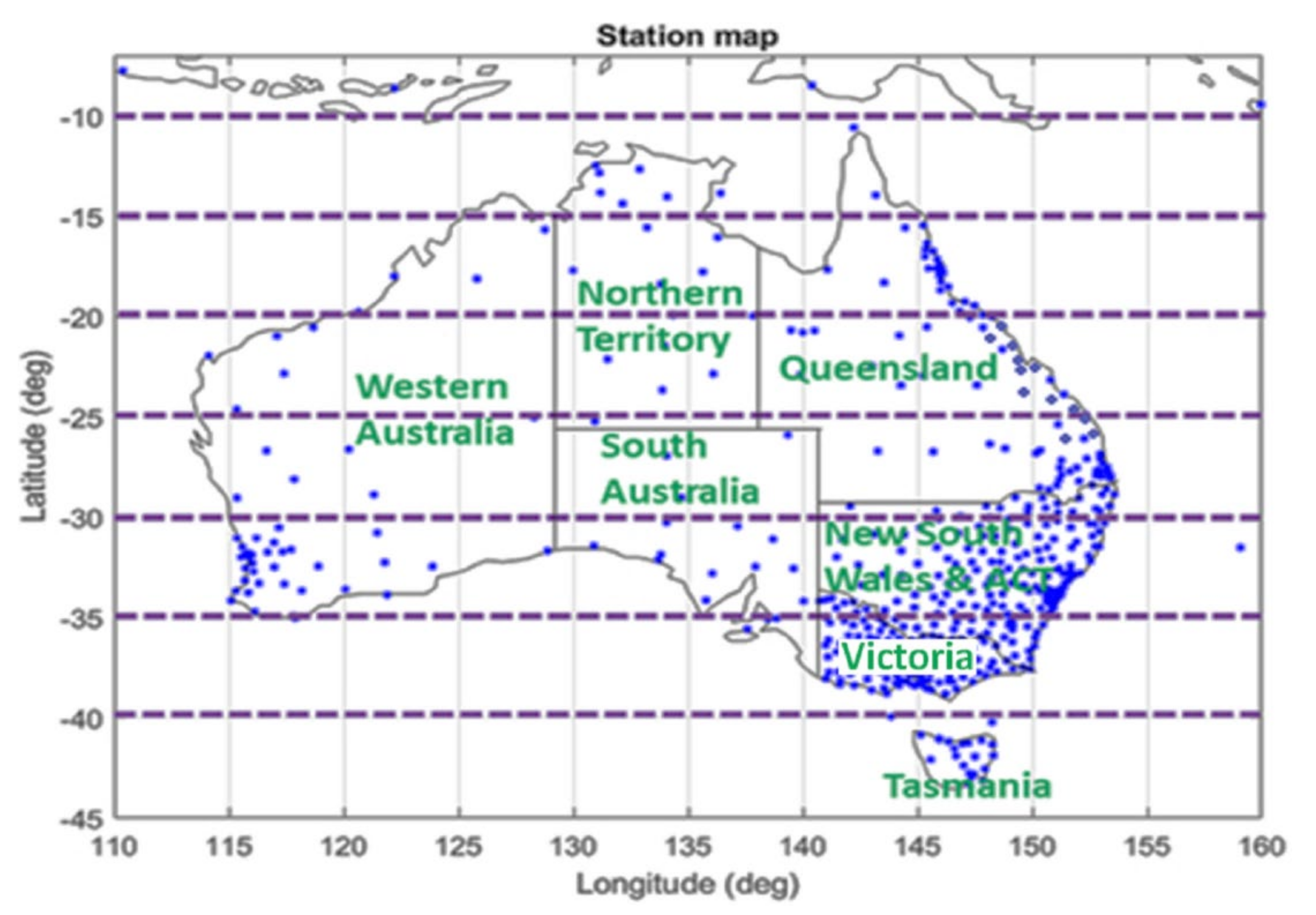
3.1. Evaluation of the Ionospheric Corrections in Different Parts of Australia

Figure 1 shows the current distribution of the Australian GNSS CORS networks along with its states and territories. As Australia has a large and sparsely populated landmass, the density of the GNSS CORS networks is not uniformly distributed. Hence, it is of interest to evaluate the achievable accuracy of a linearly interpolated ionospheric corrections model based on the existing configuration of GNSS CORS networks. Furthermore, as the ionospheric effects vary as a function of latitude, it is therefore of importance to evaluate the ionospheric corrections in different regions. A series of analyses were undertaken based on selected test regions defined by latitudinal changes from low to mid-latitudes. The width (change in latitude) of test regions was defined as 5° latitude starting from 10°S to 45°S, and the length (change in longitude) varied according to the respective test regions. In general, it varied between 8° to 12° longitude, starting from 110°E to 155°E.

More than 100 Australian CORS stations with emphasis on state-wide infrastructure networks were used to assess the latitudinal variation in the interpolated ionospheric delay corrections over Australia. An additional 70 global CORS stations were also selected to supplement and strengthen the processing model. Only GPS measurements were processed and used for estimating ionospheric corrections. An example of the geographic distribution of the selected CORS stations used is presented in Figure 2.

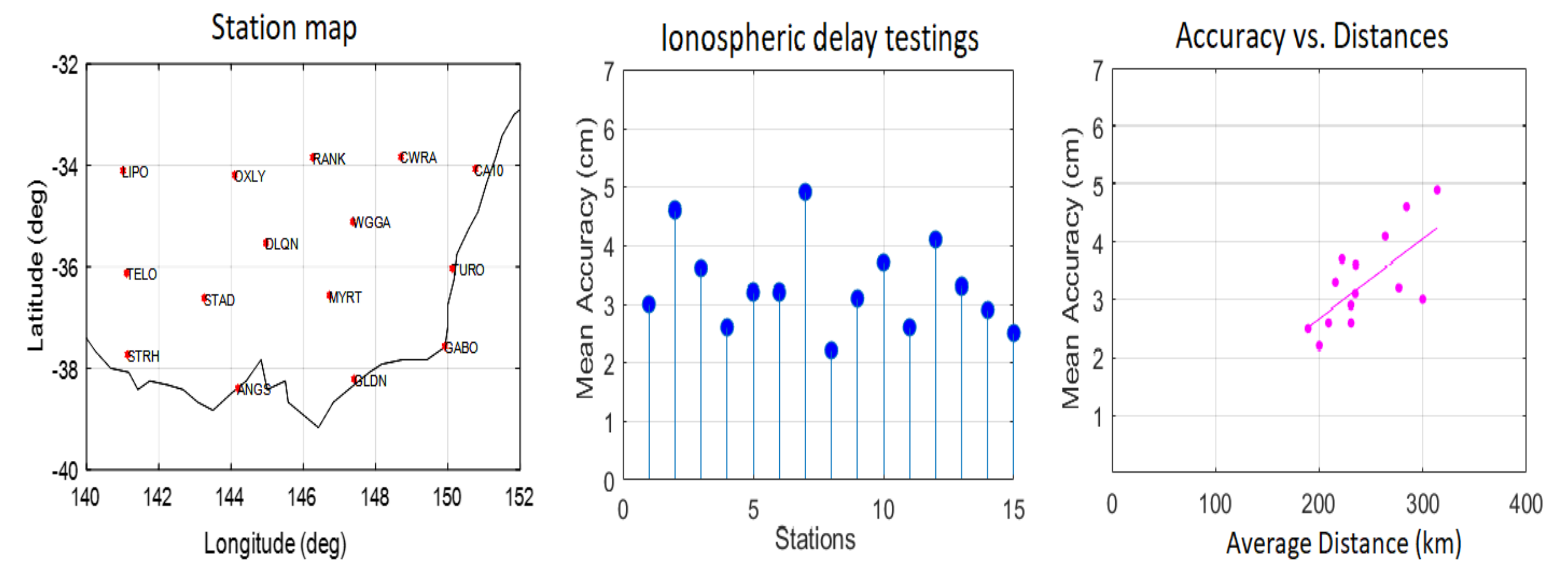
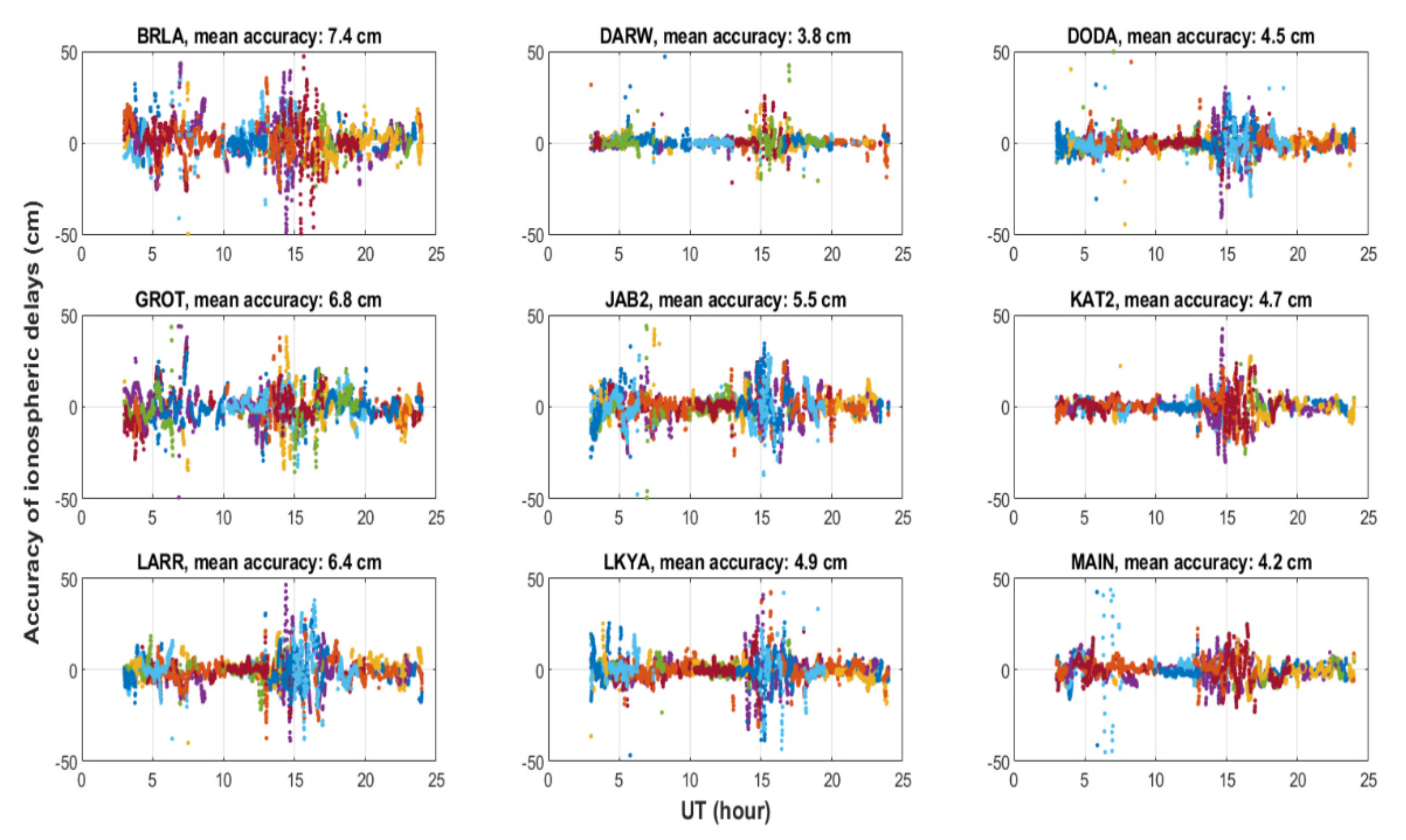
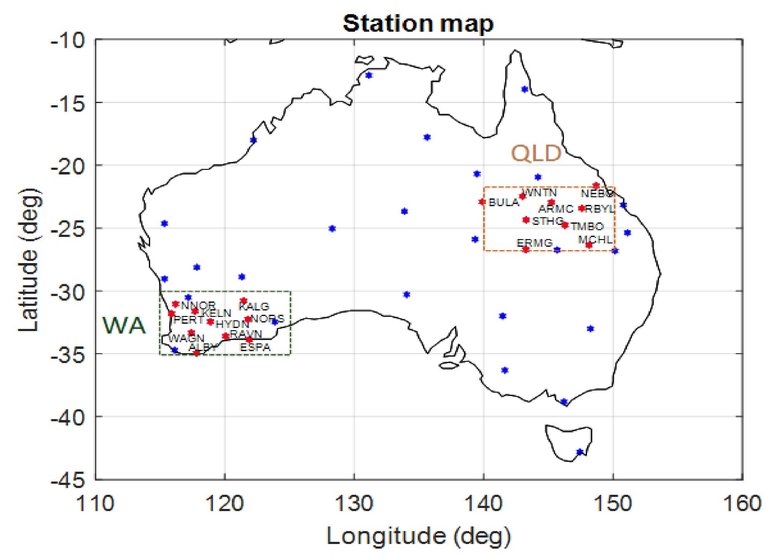
3.1.1. Victoria (VIC), New South Wales (NSW) and Canberra (ACT)

The State of Victoria is in the mid-latitude region between 34°S to 39°S. Victoria has the densest GNSS CORS network in Australia, with an average distance between stations of 80 km. One hundred and twelve state-wide Victorian stations were selected to assess the variability of the ionospheric corrections. The time series plots of the left of Figure 3 show the precision of the SD ionospheric corrections on 6 May 2021 at two Victorian CORS stations, ALBU and ANGS. The bar charts on the right of Figure 3 show the accuracy (difference) of the ionospheric model at these two stations. The accuracy was computed based on the differences between the interpolated ionospheric corrections and measured values at the evaluation CORS station. It is important to note that the measured slant ionospheric corrections at the evaluation stations were not used in generating the interpolation model. In addition, only values from 3 to 24 UT (LT = UT + 10) were considered in the evaluation, as the PPP network processing required a couple of hours for the solution to converge and stabilise. For a dense network in Victoria, a linear interpolation method of SD slant ionospheric corrections can reach an average accuracy of less than 5 cm, with a mean accuracy of 1.2 cm for ALBU station and 0.8 cm for ANGS station. There were some occasions where large variations can be found up to 10 cm, but 99% of the delay accuracy was distributed within 5 cm.

To evaluate the accuracy of the ionospheric corrections as functions of the CORS network density (e.g., average distance between station) and number of stations used in generating the ionospheric corrections, three scenarios with different CORS network configurations were simulated as shown in Figure 4a–c. The three scenarios were (a) 112 stations with an average between-station distance of 80 km; (b) 40 stations with an average between-station distance of 120 km; (c) 15 stations with an average between-station distance of 200 km. Figure 4d–f shows the mean accuracy for each station in the corresponding network. From the analysis, large differences were mainly observed at stations located at the region border and away from the network. In scenario (c), two stations (i.e., LIPO and CA10), located at the latitude of 34°S and far away from the network, showed larger differences than in scenarios (a) and (b).

To examine the relation between the mean accuracy and the position of a testing station in a regional network, we calculated an average distance from the testing station to three nearest CORS stations, herein known as the average distance. Figure 4g–i presents the accuracy as a function of the average distance of the testing station in the network. For a region of 5° latitude ×10° longitude with 112 stations (g), the ionospheric corrections accuracy of 1 to 2.5 cm can be obtained with the average distance below 80 km, whereas approximately 3 cm and 4 cm mean accuracies can be reached with average distances of approximately 100 km and up to 200 km, respectively. These values are also the same as for the network of 40 stations (h). For a network of 15 stations (i), 13 stations with an average distance around 200 to 250 km have a mean accuracy from 2 to 4 cm, whereas two CORS stations situated at the border of the test region between VIC and NSW, approximately 300 km from the three nearest stations, have a mean accuracy of up to 6 cm. Therefore, it can be concluded that the number of stations and spatial distribution play major roles in influencing the achievable accuracy of the ionospheric corrections model.

To further validate the scenario with 15 stations evenly distributed in the 5° × 10° area, it was of interest to investigate if the inclusion of additional stations around the border would strengthen the ionospheric modelling around the border region, thus improving the overall accuracy of the corrections. Figure 5 (left) is a map of 15 CORSs with 10 VIC stations plus 5 neighbouring NSW stations. In this set up, the CORSs were well distributed across the test region compared to the previous test scenarios in Figure 4c. The average distance between the testing station to the three nearest stations in this test region is from 200 to 300 km. With this network configuration, an average of 5 cm accuracy can be achieved for all stations in the local area. The NSW and ACT areas also have a dense GNSS CORS network with an average distance of 120 km and an even distribution. Using this simple interpolation, we can achieve an accuracy below 5 cm.

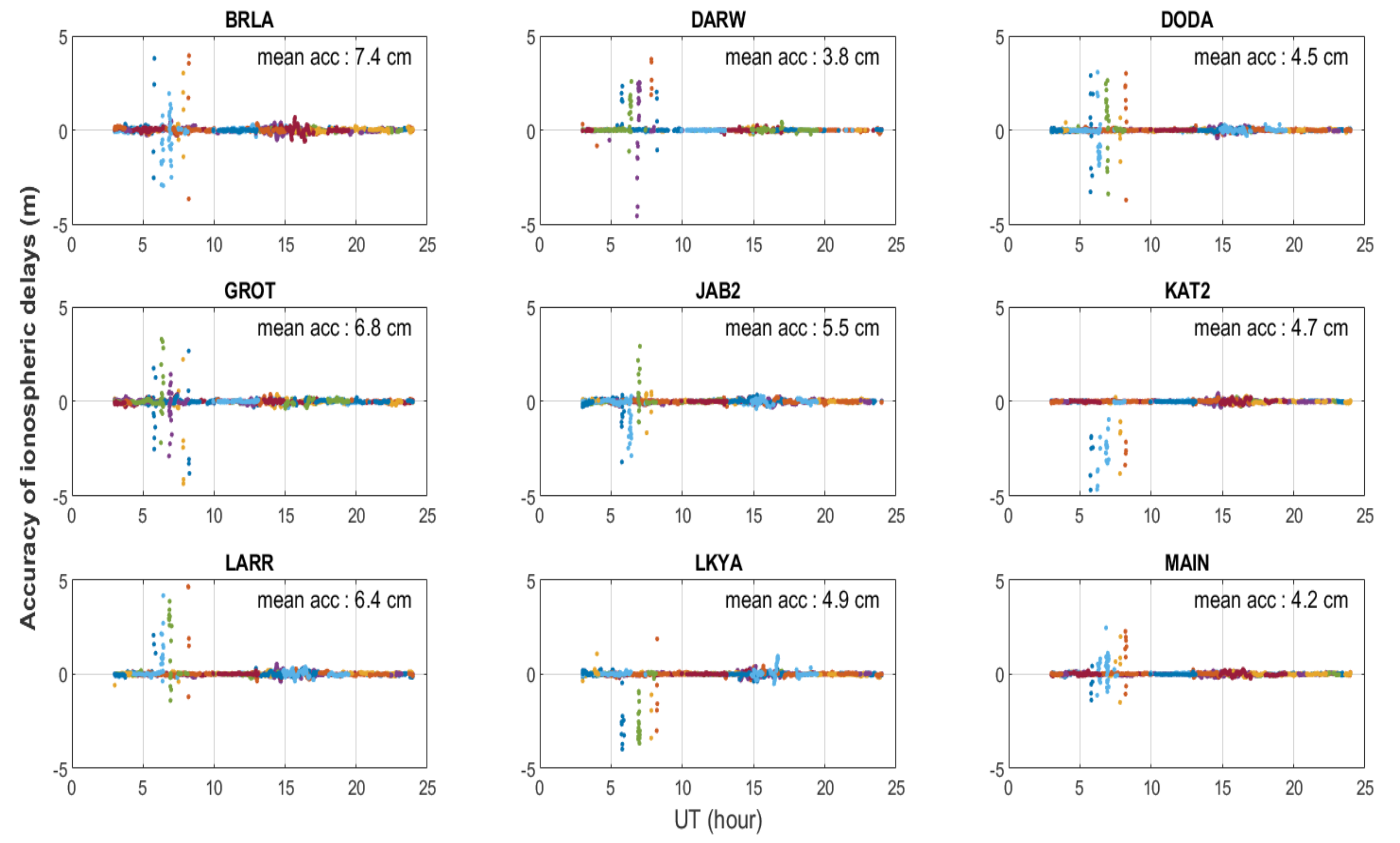
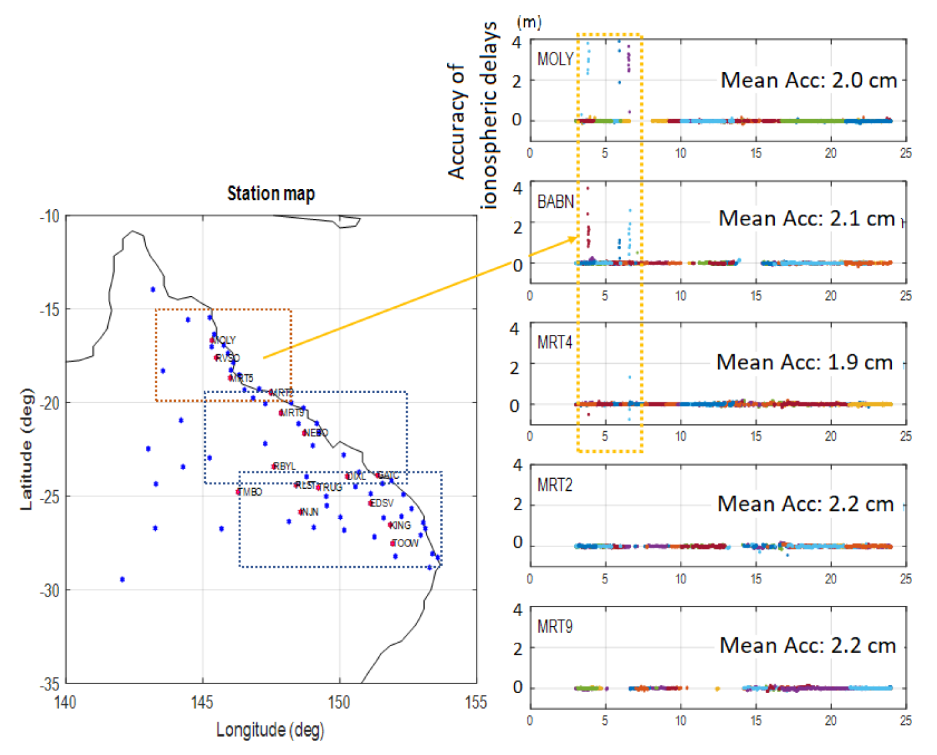
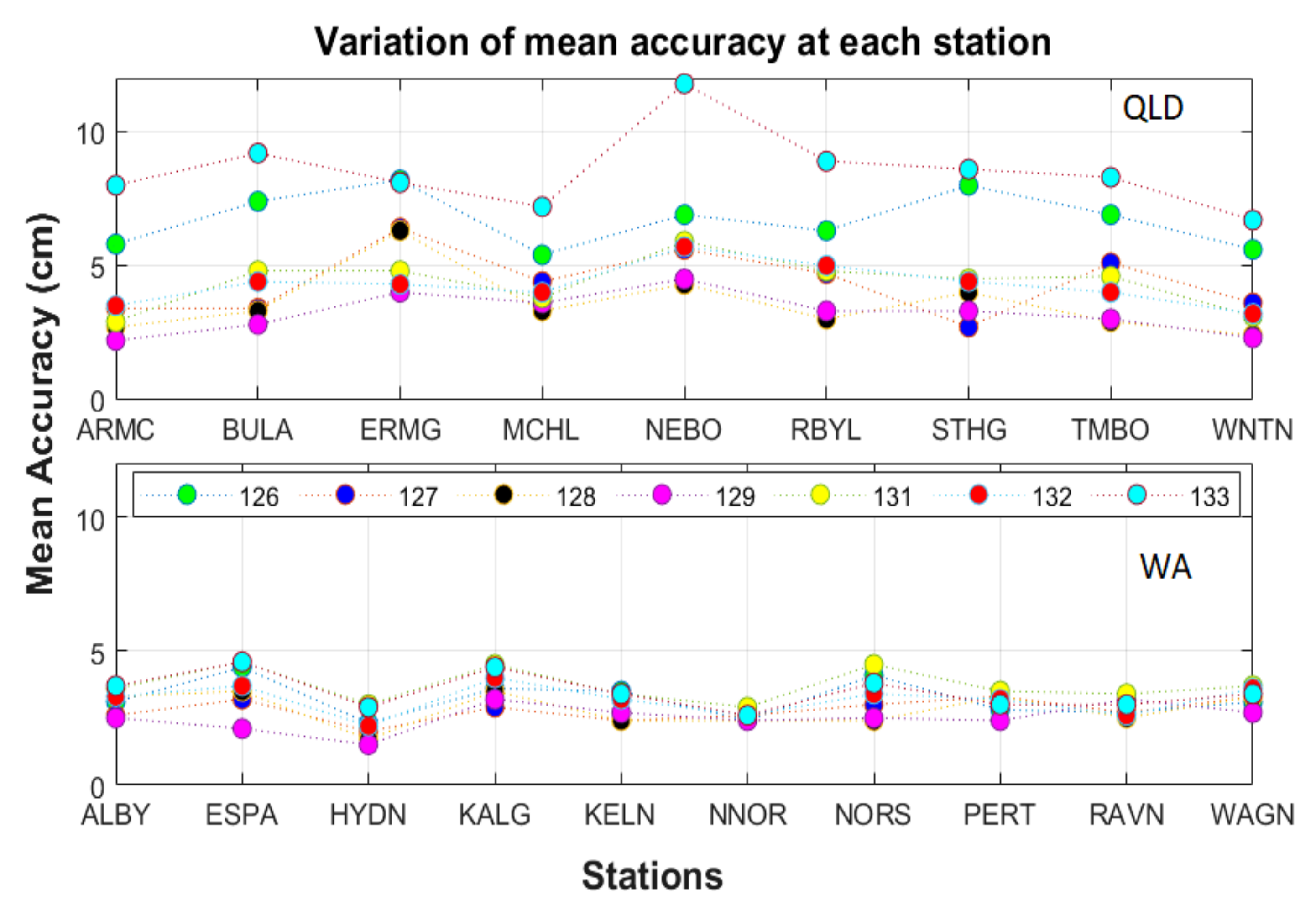
3.1.2. North Territory (NT) and East Coast of Queensland (QLD)

Northern Territory (NT) and the northern part of Queensland (QLD) are in the low-latitude region (~0° to 30°S), where the electron density is expected to be higher than the mid-latitude region. In the NT and west QLD, the GNSS networks are sparse. In fact, the majority of the GNSS stations in QLD are located along the east coast, where the population concentrates. In NT, there are approximately nine stations covering an area of 5° latitude ×8° longitude. The yellow box in Figure 6 shows the test region defined for NT.

Figure 7 shows the differences between the interpolated ionospheric corrections and the measured values for each of the nine NT CORS stations on 6 May 2021. Based on the observations on this day, all stations show a high variation of up to 5 m, particularly between 3:30 to 8 UT, corresponding to 12:00 to 17:30 LT. These high variations occurred during the afternoon, when the Equatorial Ionospheric Anomaly (EIA) is at maximum density and were observed from some GPS satellites located on the north of the testing station. This caused a large deviation since the signals of those satellites pass through the EAI, where the high electron density content is.

Upon closer inspection of the results, as shown in Figure 8 (note that the y-axis scale is in centimetres), differences of up to 50 cm are also found between 13 to 17 UT, corresponding to 22:30 to 2:30 LT. These high variations occurred around midnight LT and were observed from most GPS satellites of the testing station. This potentially indicates the effects of mid-night ionospheric density disturbance occurring in the low-latitude region, which were not present in the mid-latitude region.

To further investigate of this phenomenon, GNSS station data along the east coast of QLD were processed to evaluate and determine the latitudinal extent of these ionospheric disturbances. The testing region included a dense CORS network from 15° to 30°S within 142° to 152°E. Three test areas of 5° latitude ×5° longitude and 5° latitude ×8° longitude were defined for the QLD east coast (Figure 9), each consisting of 14 CORS stations. The red stations with IDs in Figure 9 are the testing stations used in the ionospheric corrections interpolation. A high variation in ionospheric delays can be seen at stations with latitudes of up to 20°S during these time periods; and the variation diminished as the latitude increased.

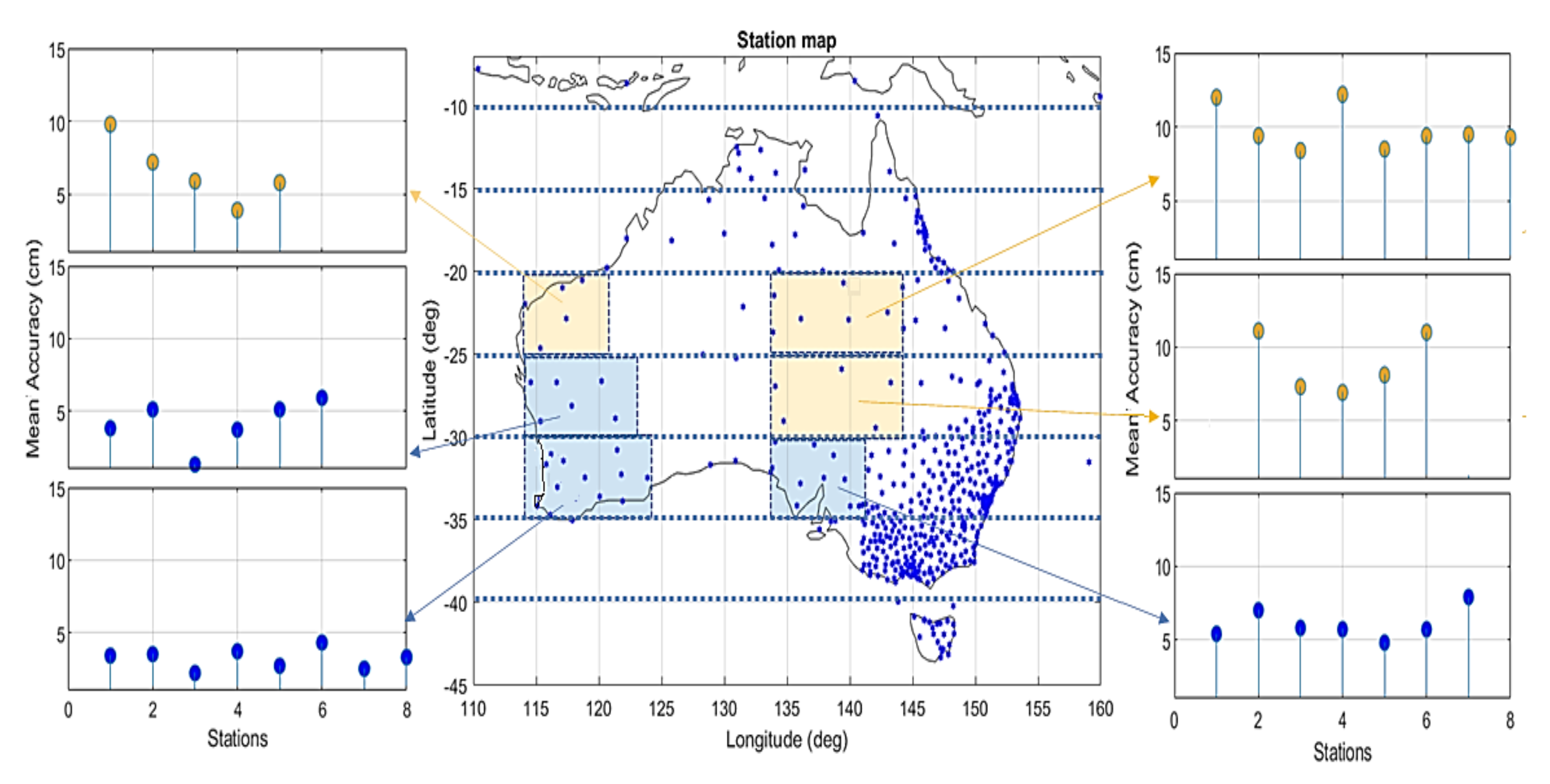
3.1.3. South Australia (SA), Western Australia (WA) and Central Australia

Additional test regions in South Australia (SA), Western Australia (WA) and Central Australia as shown in Figure 10 were selected for evaluation. Each of these test regions cover 5° latitude with a varying longitude of 8° to 10° depending on the availability of the stations’ data. Based on the results presented in this figure, the blue regions provide a higher average accuracy of less than 8 cm. The orange regions, on the other hand, give an average accuracy between 5 and 15 cm. Those accuracies correspond to the latitudes (mid/low) and the distribution of GPS stations (high/less) in the test regions.

3.2. Day-to-Day Accuracy of the Ionospheric Corrections during Ionosphere Quiet and Disturbed Days

To assess the accuracy of the ionospheric corrections for a day-to-day period, seven days of GNSS measurements from 6 to 9 May (DOY 126 to 129) and 11 to 13 May (DOY 131 to 133) 2021 were processed for two test regions in WA and QLD as shown in Figure 11. DOY 130 was excluded due to the unavailability of station data for the testing. These two test regions have a similar number and density of GNSS CORS stations and are in different latitudes.

Figure 12 shows the mean accuracy of the interpolated ionospheric corrections for QLD (top) and WA (bottom) for the seven-day study period. In the WA region, the day-to-day mean accuracy seems stable and varies within 5 cm. In QLD, a higher variation is observed in the day-to-day mean accuracy, from 2 cm to 10 cm. On DOY 133, the mean accuracy at the NEBO station reaches 12 cm and is likely caused by its location situated at the border. The reason for the differences observed in these two regions could be based on the latitude as well as the distribution of the CORS stations in that region. The QLD test region is situated in the low latitude, whereas the WA test region is in the mid-latitude. Even though the number of CORS stations used in the ionospheric corrections interpolation in two regions is similar, the WA CORS stations are located nearer to each other (approximately 120 km) compared to those of QLD (more than 200 km).

The one-week study period included a geomagnetic storm with Kp = 7 on 12 May 2021 (DOY 132). Day 132 is the most disturbed day and day 126 (6 May) is in the list of quiet days in May 2021 [24,25]. However, based on the results presented in Figure 12, it appeared that there were little differences observed in the mean accuracy. In fact, the mean accuracy on some quiet days can be higher than those on the disturbed day.

For further investigation, data from two days: one ionospheric quiet day on 6 May 2021, and one ionospheric disturbed day on 12 May 2021, and from different testing regions across Australia, were selected for comparison. The results presented in Figure 13 are for NT, WA, NSW, and VIC. From this study, no large differences in accuracy were observed between the ionospheric quiet and disturbed day. However, a larger standard deviation was observed during the disturbed day than the quiet day and, in some instances, reached 70 cm in NT, which indicates that the ionospheric delays were more varied during the disturbed period.

4. Discussion

The achievable accuracy of a local ionospheric delay model using the linear interpolation method in Australia has been evaluated to understand the impact of the ionosphere on GNSS positioning in different latitudinal regions, as well as the number and spatial density of GNSS stations in Australia. With dense CORS networks (nominal spacing of 100 km or less) in VIC, NSW and ACT, 1 to 5 cm accurate ionospheric corrections can be obtained with a simple linear interpolation ionospheric model. In fact, approximately a one-centimetre-level accuracy can be obtained most of the time if all stations in the current networks in this region are processed and used in the ionosphere modelling. Referring to Section 3.1, it was found that, with at least 15 GNSS stations (nominal spacing of 200 km and well geographically distributed) for a region of 5° latitude ×10° longitude, a mean accurate ionospheric correction within 5 cm can be obtained when a user stands on this region.

For other regions in mid latitudes, the mean accuracy obtained varied depending on the distributions of CORS stations and their availability. The mean accuracy obtained from the valuation can be around 5 cm or up to 15 cm (Figure 10). For those mid regions, the mean accuracy is not varied much for day-to-day variation. It largely depends on the spatial distribution of the station network. The linear interpolation in our method is feasible from five CORS stations. Therefore, for the testing stations with the numbers of CORS stations around 10, to maximise the achievements, some surrounding stations nearby the border of the network can be used to interpolate. Therefore, the area can be extended, not only using stations in the size of testing.

For low-latitude regions, overall, a mean accuracy of 8 cm can be obtained. However, high variations in ionospheric corrections were found during the afternoon (or daytime LT) or midnight. As presented in Section 3.2, Figure 7 shows the discrepancy of ionospheric delays during 5 to 8 UT on 6 May 2021 for some specified satellites observed at all stations. The data from those stations were further examined during the week and it was found that these variations often occurred in a low latitude from 3 to 8 UT (daytime in LT). To better understand this phenomenon, we selected the location of high variations in ionospheric delays of each satellite during daytime, which has an accuracy larger than 50 cm. It was found that those high variations occurred at the north of the testing station, where the GNSS signal paths were of a low elevation. The north side of stations at NT is the equatorial regions and NT is located in the equatorial ionospheric anomaly, so those variations may be caused by electron density irregularities that affected some receiver-satellite paths. The magnitude of those values varied day by day. Figure 14 presents the findings of two example stations, BRLA and DODA. The subplots on the top show the differences between the interpolated and measured ionospheric corrections as a function of time at BRLA and DODA on 6 May 2021, which are the same as those presented in Figure 7. The subplots on the bottom of Figure 14 are the sky paths of all GPS satellites received during 5 to 10 UT observed at the two stations. More than a 50 cm accuracy is marked by red crosses, which are in low elevations at the north of the testing station (the black asterisk at each figure).

High variations were also observed for most satellites during midnight LT as presented in Figure 8. The 50 cm deviations that occurred around midnight on 6 May could be caused by a substorm-like activity that regularly took place during quiet days [26]. Based on the SME index [27], the substorm-like activity coincided with these high variations. Wave activity, which can occur from substorm activity, such as travelling ionospheric disturbances, are often larger in amplitude in the equatorial/low-latitude region compared with the midlatitude region [28]. Therefore, these may explain the high variations observed.

The mean accuracy of the interpolated ionospheric corrections compared with the measurement was found to be comparable between the ionospheric quiet of 6 May and disturbed days in the minor storm of 12 May. However, a larger standard deviation was observed during the disturbed day than the quiet day, indicating a variability of ionospheric delays during the disturbed period in the Australian region. The impact of the storm is different globally. In this minor storm, the impact was noticed in the South American sector with 60%, whereas less impact was found in Australia [29].

From this research, the desirable size of the region/grid for the mapping of the SD ionospheric corrections using the linear interpolation of ionospheric corrections is 5° latitude ×10° longitude. This recommendation is based on the current configuration and availability of GNSS CORS networks across Australia. Continental Australia can be divided into 15 regional/local maps, labelled as 1 to 15 and marked by different colours in Figure 15.

The regions in this map can be explained as:

(1)

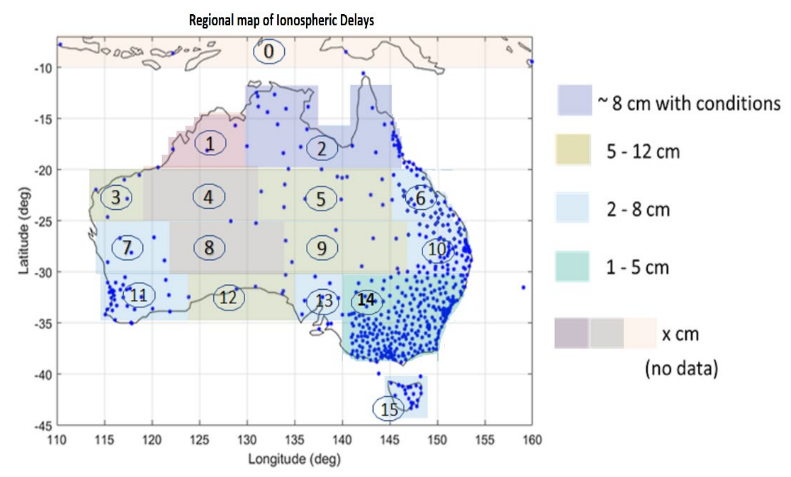
Region 0 covers multiple islands of Indonesia and there were no available GNSS stations; therefore, it is not included for analysis.

(2)

Regions 1 and 2 are in the low latitudes of 10° to 20°S, where the high electron density and the variation in the equatorial ionospheric anomaly are found. The ionospheric corrections around midnight or low-elevation GNSS satellites below 20 deg during daytime can be high. With the current available CORS networks in NT and northern QLD, 8 cm level ionospheric corrections can be obtained in Region 2, while additional GNSS stations will be required to be installed in Region 1 (northern WA) if centimetre-level accurate ionospheric corrections will be needed in this area.

(3)

Regions 3, 5, 9 and 12 are in the mid latitudes from approximately 20° to 35°S. The mid-latitude regions were less impacted by equatorial ionospheric disturbances. In these regions, the current available GNSS CORS networks are sparse. Nevertheless, it was found that 5 to 12 cm level accurate ionospheric corrections can be obtained in these regions. In the eastern corner of WA, where the borders of SA and NT meet, i.e., Regions 4 and 8, no evaluation was undertaken due to an insufficient number of GNSS stations.

(4)

Regions 6, 7, 10, 11, 13, 14 and 15 are also in the mid latitudes covering 20° to 45°S. For these regions, a high number and dense CORS networks exist. Therefore, the average obtainable accuracy of the ionospheric corrections is within 2 to 8 cm.

This map is a reference based on the temporal valuable data in different regions in Australia. The precise accuracy may change based on the number of CORS station networks and the availability of data in each region. However, we can basically estimate how good the ionospheric delays are using a simple interpolation of the local network compared to the real measurement.

5. Conclusions

The aim of this research was to assess the achievable accuracy of a local ionospheric delay model for Australia using the linear interpolation method. The assessment was conducted by taking into consideration the impact of the ionosphere in different latitudinal regions, i.e., low and mid latitudes, as well as the number and spatial density of the GNSS CORS networks that exist in Australia. To summarise, local/regional ionospheric modelling using the linear interpolation method can produce the centimetre-level accurate ionospheric correction required for high-accuracy GNSS positioning. Based on our observations, centimetre-level accurate ionospheric corrections can be achieved if there are sufficiently dense (i.e., nominal spacing of approximately 200 km) GNSS CORS networks in the region. The achievable accuracy could be dependent on the latitudinal region (i.e., low or mid latitude) and the time of day, as well as the number and spatial density of the GNSS CORS network. For a large geographic country like Australia where CORS networks are not uniformly distributed, consideration for CORS network investment will mainly depend on the socioeconomic benefits and return of investment. To obtain centimetre-level ionospheric corrections across Australia using a simple linear interpolation, we propose a framework of 15 regional ionospheric maps of 5° latitude ×10° longitude with a minimum of 15 CORS stations in each map region to cover continental Australia.

References

1. Choy, S.; Zhang, K.; Silcock, D. An Evaluation of Various Ionospheric Error Mitigation Methods used in Single Frequency PPP. Positioning 2008, 1, 62–71. [Google Scholar] [CrossRef] [Green Version]
2. Choy, S.; Bisnath, S.; Rizos, C. Uncovering common misconceptions in GNSS Precise Point Positioning and its future prospect. GPS Solut. 2016, 21, 13–22. [Google Scholar] [CrossRef]
3. Choy, S. High accuracy precise point positioning using a single frequency GPS receiver. J. Appl. Geod. 2011, 5, 59–69. [Google Scholar] [CrossRef]
4. Zumberge, J.F.; Heflin, M.B.; Jefferson, D.C.; Watkins, M.M.; Webb, F.H. Precise point positioning for the efficient and robust analysis of GPS data from large networks. J. Geophys. Res. 1997, 102, 5005–5017. [Google Scholar] [CrossRef] [Green Version]
5. Kouba, J.; Héroux, P. Precise point positioning using IGS orbit and clock products. GPS Solut. 2001, 5, 12–28. [Google Scholar] [CrossRef]
6. Samper, M.D.; Merino, M.M. Advantages and Drawbacks of the Precise Point Positioning (PPP) Technique for Earthquake, Tsunami Prediction and Monitoring. In Proceedings of the ION 2013 Pacific PNT Meeting, Honolulu, HI, USA, 25 April 2013; pp. 9–26. [Google Scholar]
7. Wabbena, G.; Schmitz, M.; Bagge, A. PPP-RTK: Precise Point Positioning Using State-Space Representation in RTK Networks. In Proceedings of the 18th International Technical Meeting of the Satellite Division of The Institute of Navigation (ION GNSS 2005), Long Beach, CA, USA, 16 September 2005; pp. 2584–2594. [Google Scholar]
8. Leick, A.; Rapoport, L.; Tatarnikov, D. GPS Satellite Surveying; John Wiley & Sons: Hoboken, NJ, USA, 2015. [Google Scholar]
9. Alkan, R.M.; Erol, S.; Ozulu, I.M.; Ilci, V. Accuracy comparison of post-processed PPP and real-time absolute positioning techniques. Geomat. Nat. Hazards Risk 2020, 11, 178–190. [Google Scholar] [CrossRef]
10. Rovira-Garcia, A.; Juan, J.M.; Sanz, J.; González-Casado, G.; Bertran, E. Fast Precise Point Positioning: A System to Provide Corrections for Single and Multi-frequency Navigation. J. Inst. Navig. 2016, 63, 231–247. [Google Scholar] [CrossRef] [Green Version]
11. Juan, J.M.; Hernández-Pajares, M.; Sanz, J.; Ramos-Bosch, P.; Aragon-Angel, A.; Orus, R.; Ochieng, W.; Feng, S.; Jofre, M.; Coutinho, P.; et al. Enhanced Precise Point Positioning for GNSS Users. IEEE Trans. Geosci. Remote Sens. 2012, 50, 4213–4222. [Google Scholar] [CrossRef]
12. Psychas, D.; Verhagen, S.; Liu, X.; Memarzadeh, Y.; Visser, H. Assessment of ionospheric corrections for PPP-RTK using regional ionosphere modelling. Meas. Sci. Technol. 2019, 30, 014001. [Google Scholar] [CrossRef] [Green Version]
13. Li, X.; Zhang, X.; Ge, M. Regional reference network augmented precise point positioning for instantaneous ambiguity resolution. J. Geod. 2011, 85, 151–158. [Google Scholar] [CrossRef]
14. Hernández-Pajares, M.; Juan, J.M.; Sanz, J.; Orus, R.; Garcia-Rigo, A.; Feltens, J.; Komjathy, A.; Schaer, S.C.; Krankowski, A. The IGS VTEC maps: A reliable source of ionospheric information since 1998. J. Geod. 2011, 83, 263–275. [Google Scholar] [CrossRef]
15. Rovira-Garcia, A.; Juan, J.M.; Sanz, J.; González-Casado, G.; Ibáñez, D. Accuracy of ionospheric models used in GNSS and SBAS: Methodology and analysis. J. Geod. 2016, 90, 229–240. [Google Scholar] [CrossRef]
16. Banville, S.; Collins, P.; Zhang, W.; Langley, R.B. Global and regional ionospheric corrections for faster PPP convergence. J. Inst. Navig. 2014, 61, 115–124. [Google Scholar] [CrossRef]
17. Choy, S.; Harima, K. Satellite delivery of high-accuracy GNSS precise point positioning service: An overview for Australia. J. Spat. Sci. 2019, 64, 197–208. [Google Scholar] [CrossRef]
18. Brown, N.; Dawson, J.; Ruddick, R. Positioning Australia for the Future. Engineering 2020, 6, 857–859. [Google Scholar] [CrossRef]
19. Harima, K.; Choy, S.; Elneser, L.; Kogure, S. Local augmentation to wide area PPP systems: A case study in Victoria, Australia. In Proceedings of the IGNSS Conference, Sydney, Australia, 6–8 December 2016. [Google Scholar]
20. Melbourne, W. The case for ranging in GPS based geodetic systems. In Proceedings of the 1st International Symposium on Precise Positioning with the Global Positioning System, Rockville, MD, USA, 15–19 April 1985; pp. 373–386. [Google Scholar]
21. Wübbena, G. Software developments for geodetic positioning with GPS using TI 4100 code and carrier measurements. In Proceedings of the 1st International Symposium on Precise Positioning with the Global Positioning System, Rockville, MD, USA, 15–19 April 1985; pp. 403–412. [Google Scholar]
22. Subirana, J.S.; Zornoza, J.J.; Hernández-Pajares, M. Detector Based in Code and Carrier Phase Data: The Melburne–Wübbena Combination. ESA Navipedia. Available online: https://gssc.esa.int/navipedia/index.php/Detector_based_in_code_and_carrier_phase_data:_The_Melbourne-W%C3%BCbbena_combination (accessed on 12 April 2022).
23. The PEA Packet. Available online: https://bitbucket.org/geoscienceaustralia/pea/src/master/ (accessed on 15 June 2021).
24. Johnston, H.F. Mean, K-Indices from Twenty-One Magnetic Observatories and Five Quiet Days and Five Disturbed Days for 1942. Terr. Magn. Atmos. Electr. 1943, 47, 219. [Google Scholar] [CrossRef]
25. The International 5 and 10 Quietest and 5 Most Disturbed Days in Each Month. Available online: https://wdc.kugi.kyoto-u.ac.jp/qddays/ (accessed on 15 April 2022).
26. Newell, T.P.; Gjerloev, J.W. Evaluation of SuperMAG auroral electrojet indices as indicators of substorms and auroral power. J. Geophys. Res. 2011, 116, A12211. [Google Scholar] [CrossRef]
27. Gjerloev, J.W. The SuperMAG data processing technique. J. Geophys. Res. 2012, 117, A09213. [Google Scholar] [CrossRef]
28. Pradipta, R.; Valladares, C.E.; Carter, B.A.; Doherty, P.H. Interhemispheric propagation and in-teractions of auroral traveling ionospheric disturbances near the equator. J. Geophys. Res. Space Phys. 2016, 121, 2462–2474. [Google Scholar] [CrossRef] [Green Version]
29. Valdés-Abreu, J.C.; Diaz, M.A.; Báez, J.C.; Stable-Sánchez, Y. Effects of the 12 May 2021 Geomgagnetic Storm on Georeferencing Precision. Remote Sens. 2022, 14, 38. [Google Scholar] [CrossRef]
Figure 1. A map showing the geographical distribution of the Australian GNSS CORS networks (blue point). The test regions have a latitudinal width of 5° north south, whereas the longitudinal length varies between 8 to 12° east west.
Remotesensing 14 02463 g001
Figure 2. A map showing the geographical distribution of the GNSS stations (red aasterisks) used to compute the ionospheric corrections for the Victoria region. Respective statewide CORS stations in New South Wales (NSW), Australian Capital Territory (ACT), Western Australia (WA), North Territory (NT), Queensland (QLD) and South Australia (SA) were used to derive ionospheric corrections for those regions.
Remotesensing 14 02463 g002
Figure 3. Results of the slant ionospheric corrections comparison at two Victorian CORS stations, ALBU and ANGS on 6 May 2021. (Left) Time series plots showing the precision (mean accuracy) of the SD slant ionospheric corrections of each satellite-receiver path based on linear interpolation method. (Right) Bar charts showing the accuracy (difference between the estimated and interpolated values) and distribution of the accuracy.
Remotesensing 14 02463 g003
Figure 4. (Top: ac) Three test scenarios in Victoria to assess the relation between the accuracy of the interpolated ionospheric corrections as function of the density of the CORS network configurations. The orange rectangles show the test area of 5° latitude ×10° longitude, and the red asterisks present for the CORS stations. (Middle: df) Plots showing the mean accuracy for each station in the corresponding network. (Bottom: gi) Plots showing the accuracy of the interpolated ionospheric corrections as a function of the average separation distance between the testing station and its three nearest stations in the local network.
Remotesensing 14 02463 g004
Figure 5. (Left) Maps of 15 CORS stations including names of ten stations in VIC and five stations (CWRA, RANK, WGGA, DLQN and OXLY) from the neighbouring NSW. The red asterisks present coordinates of those stations. (Middle) The average accuracy of the interpolated ionospheric corrections for each station on 6 May 2021. (Right) The accuracy as a function of the average separation distance of the testing station to the three nearest stations in the network, same as Figure 4.
Remotesensing 14 02463 g005
Figure 6. Map showing the GNSS CORS stations (red stars) in NT and QLD. The yellow box indicated the nominated test region for NT.
Remotesensing 14 02463 g006
Figure 7. Plots showing the differences between the interpolated and measured ionospheric corrections as function of time at the nine NT CORS GNSS stations on 6 May 2021. The colours represent for different satellite observations.
Remotesensing 14 02463 g007
Figure 8. Plots showing the differences between the interpolated and measured ionospheric corrections as function of time at the nine NT CORS GNSS stations on 6 May 2021. This figure is the same as Figure 7, but the y-axis scale is decreased from 5 m to 50 cm.
Remotesensing 14 02463 g008
Figure 9. Plots showing the differences between the interpolated and measured ionospheric corrections as a function of time at some testing stations on 6 May 2021. The dash boxed in the station map show three testing areas. The red stations with names on the station map are the testing stations. The colours in the right boxes represent for different satellite observations. The dash-orange rectangle indicates some high variation in ionospheric delays.
Remotesensing 14 02463 g009
Figure 10. Evaluation of the accuracy of the ionospheric corrections in the test regions of South Australia (SA), Western Australia (WA) and Central Australia. The blue and orange boxes show the testing regions where the mean accuracy achieved is below 8 cm and up to 15 cm, respectively. The arrows link from the testing stations to the corresponding figures of mean accuracy of each station in the test region.
Remotesensing 14 02463 g010
Figure 11. Two long-term testing areas in WA and QLD (dash boxes). The red stars are testing stations in each region. The blue stars are stations around Australia processed with PEA. Note that 15 stations around and inside the boxes were used for conducting interpolation at each testing region.
Remotesensing 14 02463 g011
Figure 12. The mean accuracy of the interpolated ionospheric corrections for the testing stations at QLD (top) and WA (bottom) during 6 to 9 May (DOY 126 to 129) and 11 to 13 May (DOY 131 to 133) 2021.
Remotesensing 14 02463 g012
Figure 13. Comparison of average accuracy in quiet day (Q on 6 May 2021) and disturbance day (D on 12 May 2021). The blue and red markers show the mean accuracy of the testing stations, whereas the green and pink stars present the standard deviation of the accuracy on the quiet and disturbance day, respectively.
Remotesensing 14 02463 g013
Figure 14. (Top) The differences between the interpolated and measured ionospheric corrections as a function of time of stations BRLA and DODA on 6 May 2021. (Bottom) The sky paths of all satellites received during 5 to 10 UT observed by BRLA and DODA stations. The line colours represent each GPS satellite. The red crosses show an accuracy higher than 50 cm. The black asterisk at each figure shows the location of testing station BRLA or DODA.
Remotesensing 14 02463 g014
Figure 15. A map showing the recommended regions for mapping of the SD ionospheric corrections and the achievable accuracy using a simple linear interpolation method. The blue dots represent CORS stations in our testing. The labels of 1 to 15 describe 15 regional maps that are divided based on the available testing stations.
Remotesensing 14 02463 g015
Publisher’s Note: MDPI stays neutral with regard to jurisdictional claims in published maps and institutional affiliations.