Funding
This research was funded by the National Key R&D Program of China, grant number 2018YFB2100501, the Fundamental Research Funds for the Central Universities, grant number 2042021kf0007, the open grants of the state key laboratory of severe weather, grant number 2021LASW-A17, the Open Fund of Hubei Luojia Laboratory, grant number 220100009, the Shenzhen Science and technology Innovation Key project, grant number JCYJ20200109150833977, in part by the National Natural Science Foundation of China under Grants 42090012, Sichuan Science and Technology Program, grant number 2022YFN0031, Zhuhai industry university research cooperation project of China, grant number ZH22017001210098PWC, 03 special research and 5G project of Jiangxi Province in China, grant number 20212ABC03A09, and Zhizhuo Research Fund on Spatial-Temporal Artificial Intelligence, grant number ZZJJ202202. The authors would like to thank the anonymous reviewers and editors for their comments, which helped us improve this article significantly.
Figure 1.
The geographical location of the study area and the DEM of the study area (according to the China basic geographic information, 2008 version).
Figure 1.
The geographical location of the study area and the DEM of the study area (according to the China basic geographic information, 2008 version).
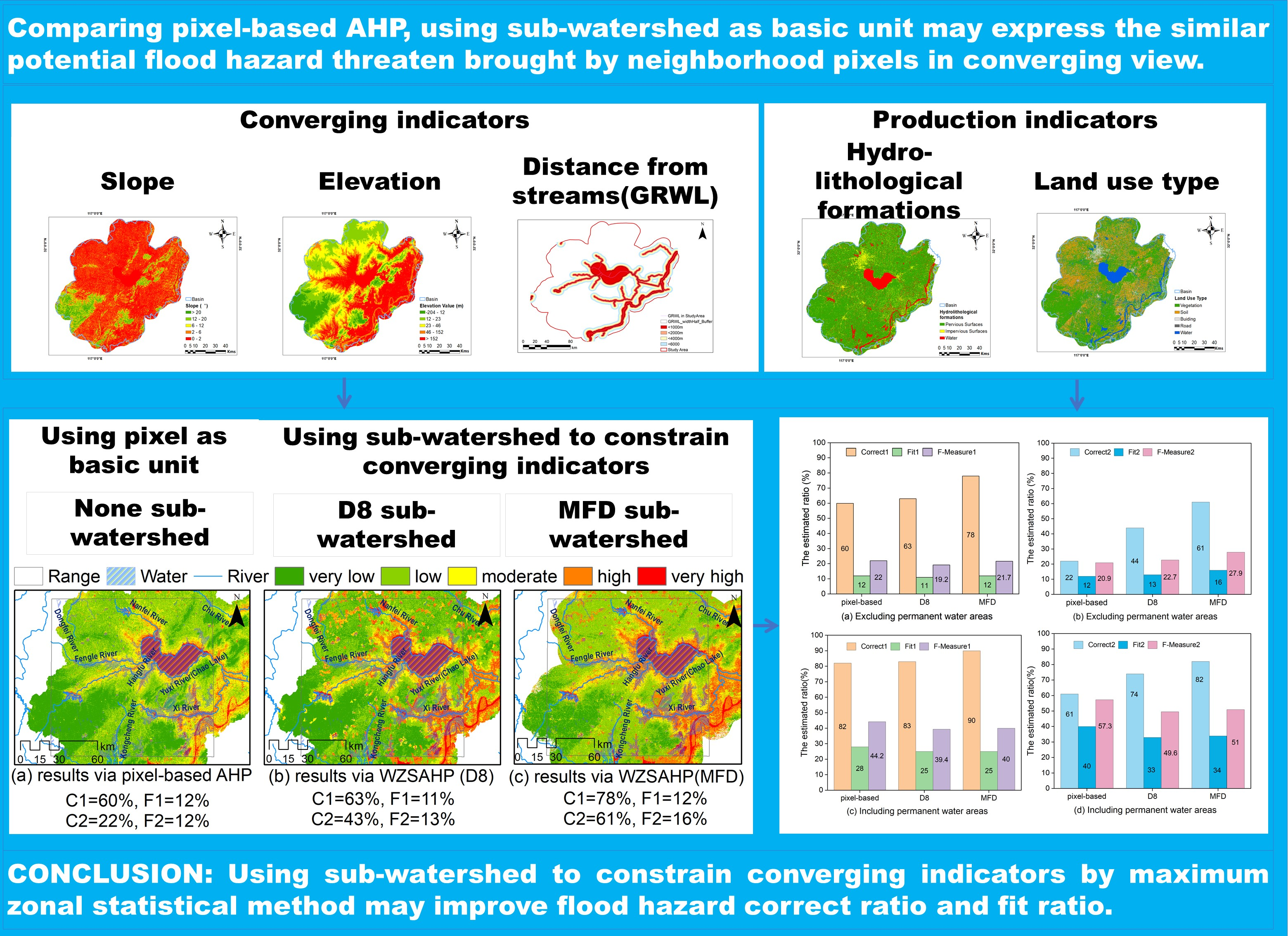
Figure 2.
The overall workflow of our study.
Figure 2.
The overall workflow of our study.
Figure 3.
The logical structure of flood hazard estimation methods: (a) The general structure of AHP, (b,c) are diagrams of ordinary AHP and WZSAHP-RC.
Figure 3.
The logical structure of flood hazard estimation methods: (a) The general structure of AHP, (b,c) are diagrams of ordinary AHP and WZSAHP-RC.
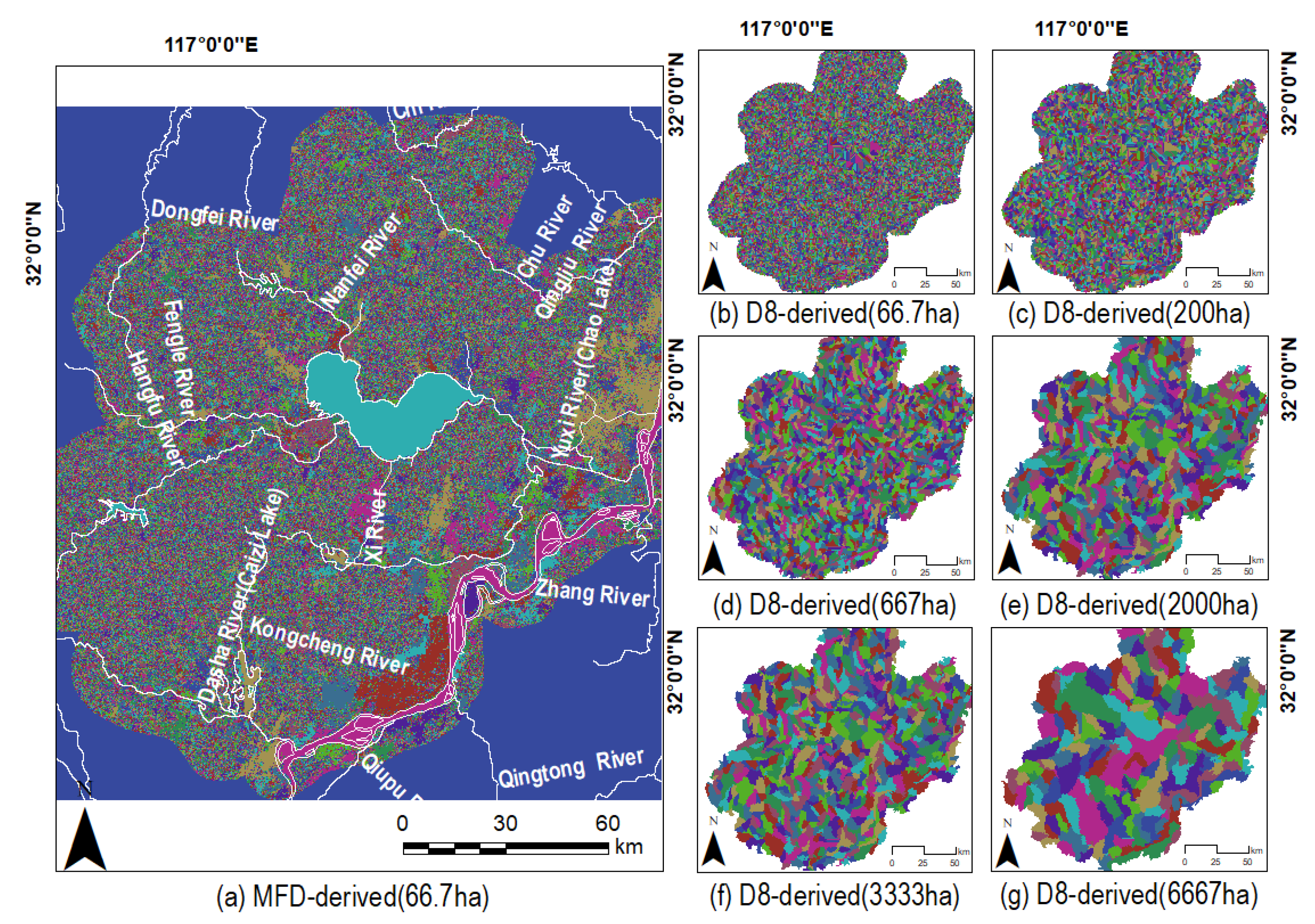
Figure 4.
The sub-watersheds derived via MFD (a) and D8 (b–g). The area threshold used in the MFD-derived subwatershed is 66.7 ha, and the area thresholds used in the D8-derived subwatershed as shown in (b–g) are 66.7 ha, 200.0 ha, 667.0 ha, 2000.0 ha, 3333.0 ha and 6667.0 ha, respectively.
Figure 4.
The sub-watersheds derived via MFD (a) and D8 (b–g). The area threshold used in the MFD-derived subwatershed is 66.7 ha, and the area thresholds used in the D8-derived subwatershed as shown in (b–g) are 66.7 ha, 200.0 ha, 667.0 ha, 2000.0 ha, 3333.0 ha and 6667.0 ha, respectively.
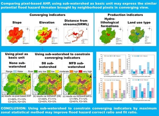
Figure 5.
The flood hazard distribution is derived from the proposed method. Subfigure (a) was the real-world flooded areas extracted by remote sensing in July 2020 in the Chaohu basin. Subfigure (b) was the flood hazard distribution estimated by the proposed model. Subfigure (c) was the detailed hazard view of the Fengle river and the Hangfu River, and subfigure (d) was the clear hazard view of the Xi River.
Figure 6.
Differences in ground-truthing flooded areas compared with expected flooded areas from the AHP and the proposed model. (a) was the distribution of validation flood area, (b) was from the original pixel-based AHP, while (c) was from the proposed model.
Figure 6.
Differences in ground-truthing flooded areas compared with expected flooded areas from the AHP and the proposed model. (a) was the distribution of validation flood area, (b) was from the original pixel-based AHP, while (c) was from the proposed model.
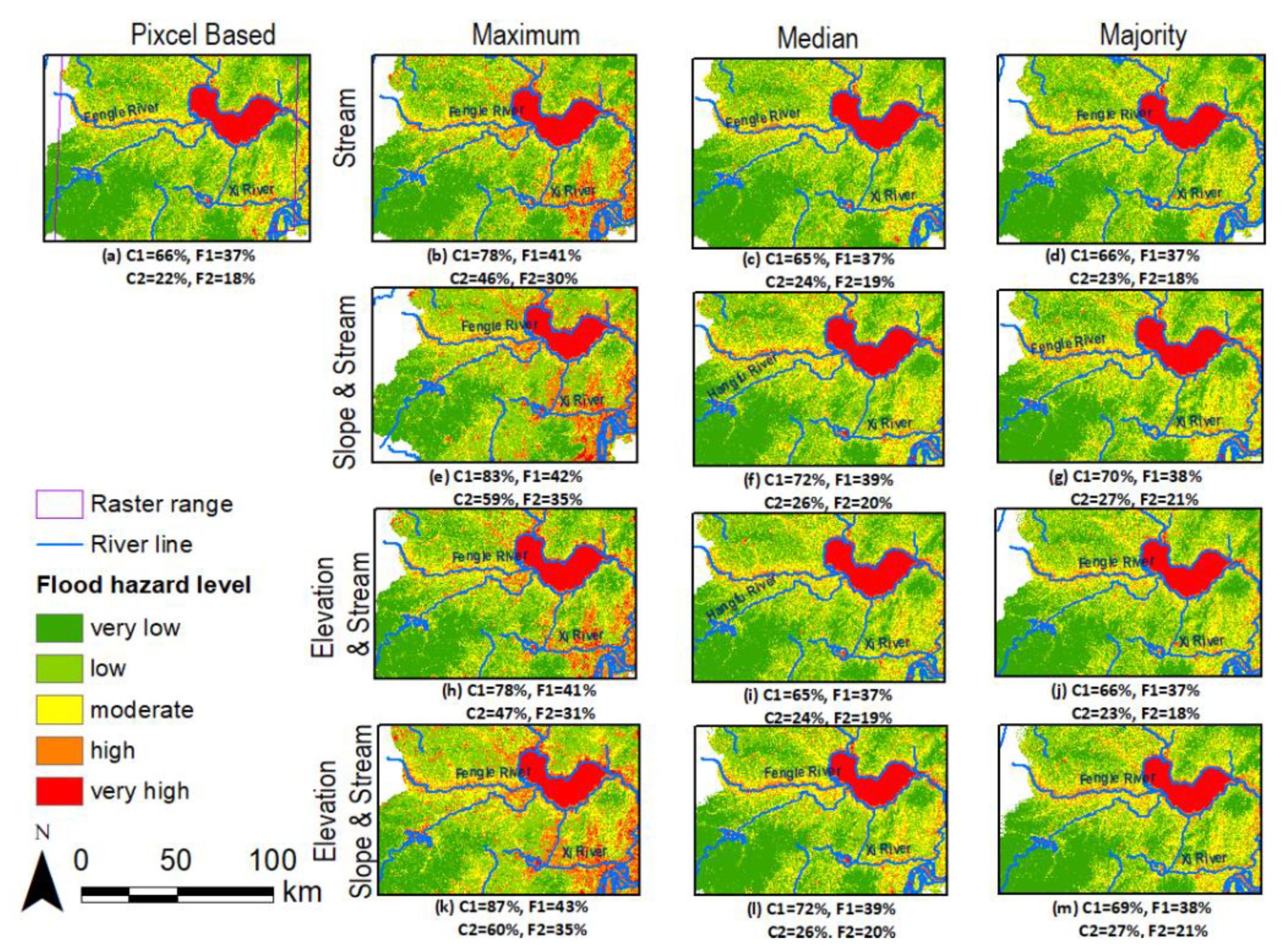
Figure 7.
Flood hazard levels from pixel-based AHP (a), while (b–m) show flood hazard levels derived by WZSAHP-RC using different indicators and zonal statistics.
Figure 7.
Flood hazard levels from pixel-based AHP (a), while (b–m) show flood hazard levels derived by WZSAHP-RC using different indicators and zonal statistics.
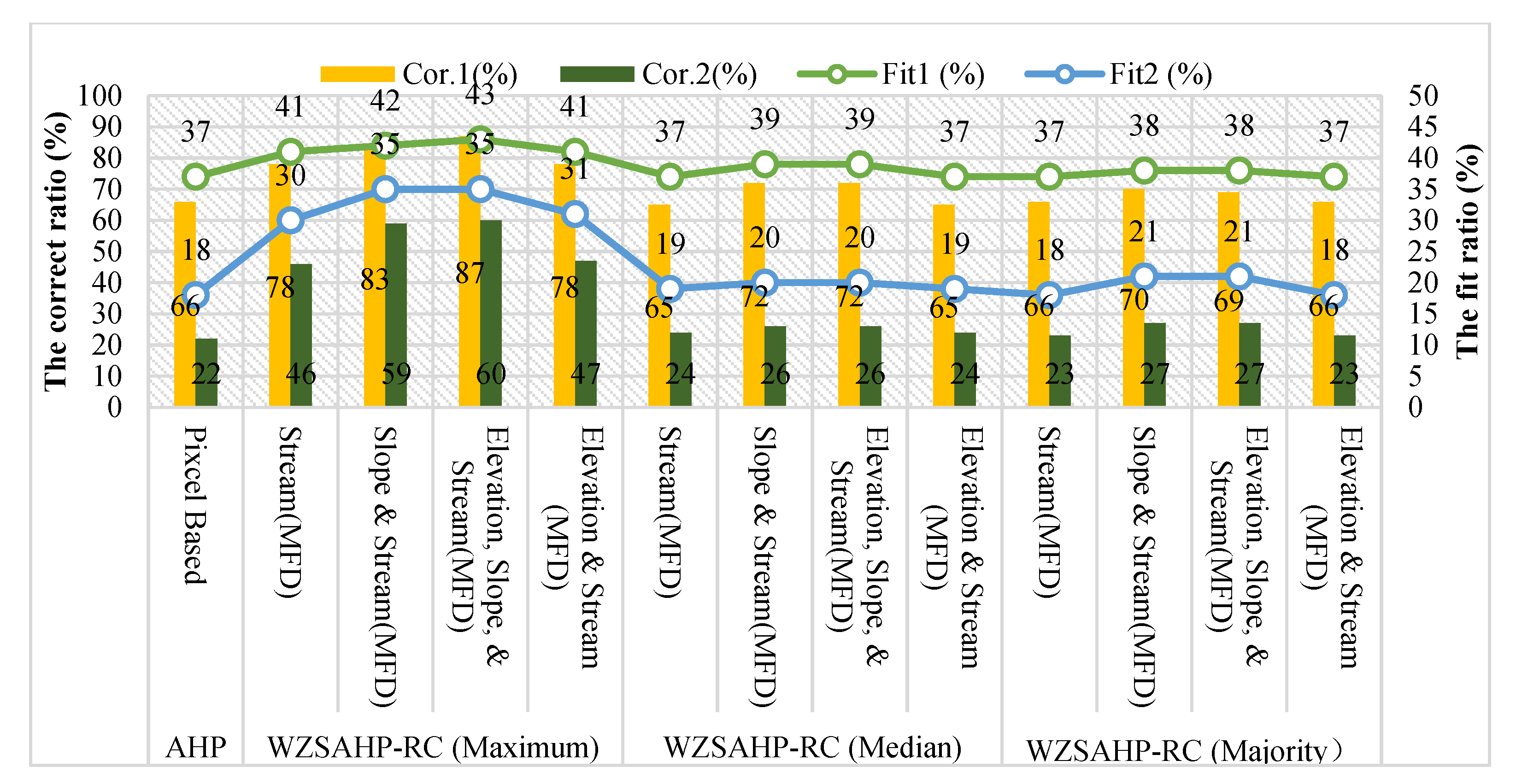
Figure 8.
The correct ratio and fit ratio values of pixel-based AHP and sub-watershed-based WZSAHP-RC models constrain different kinds of converging related indicators.
Figure 8.
The correct ratio and fit ratio values of pixel-based AHP and sub-watershed-based WZSAHP-RC models constrain different kinds of converging related indicators.
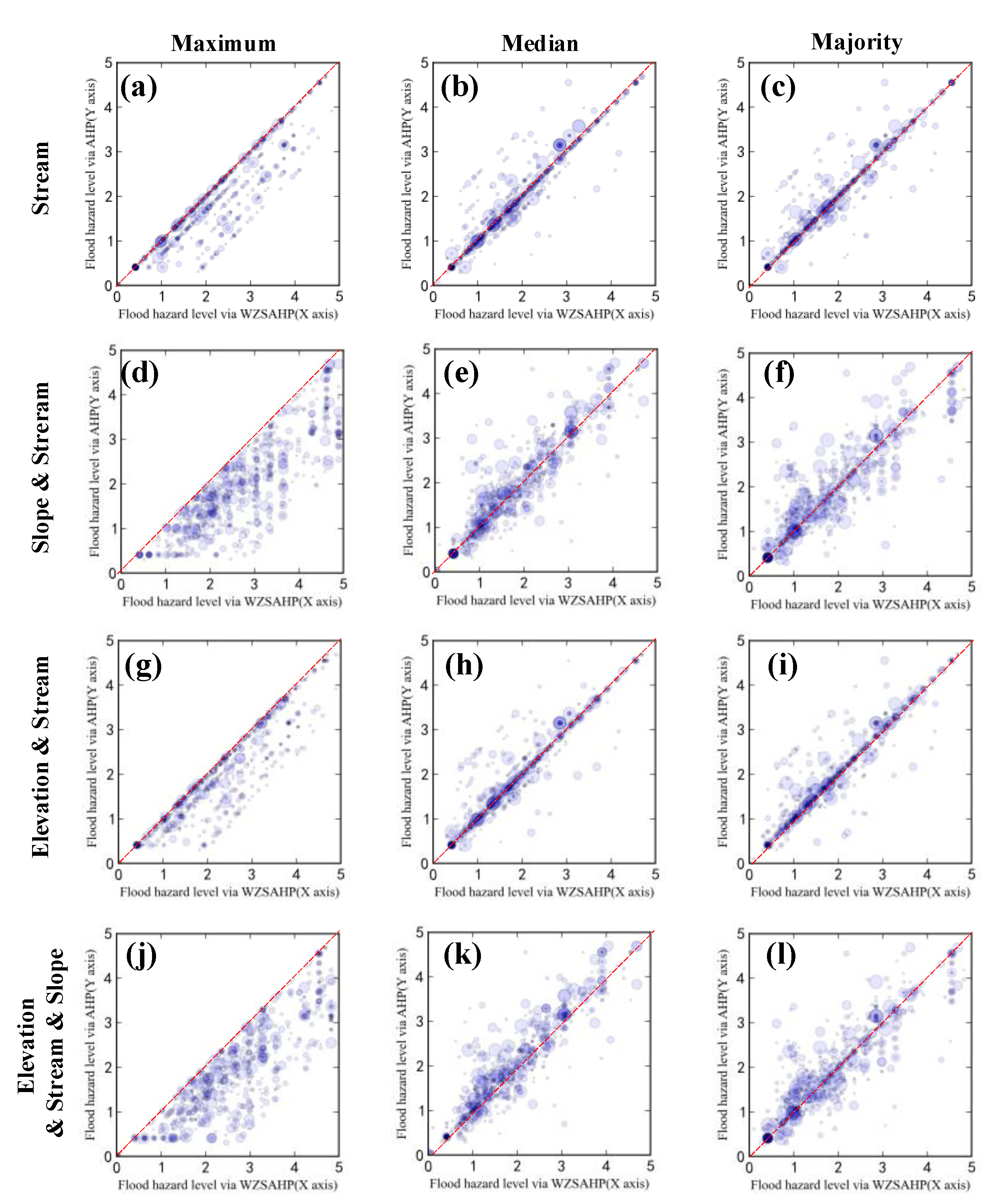
Figure 9.
Scatter diagrams of flood hazard index derived by WZSAHP-RC via MFD delimitated sub-watershed as X-axis and flood hazard index derived by AHP as Y-axis. The converged indicator in (a–c), (d–f), (g–i), and (j–l) were the same, and the sub-figures in the same column used the same type of zonal statistical method.
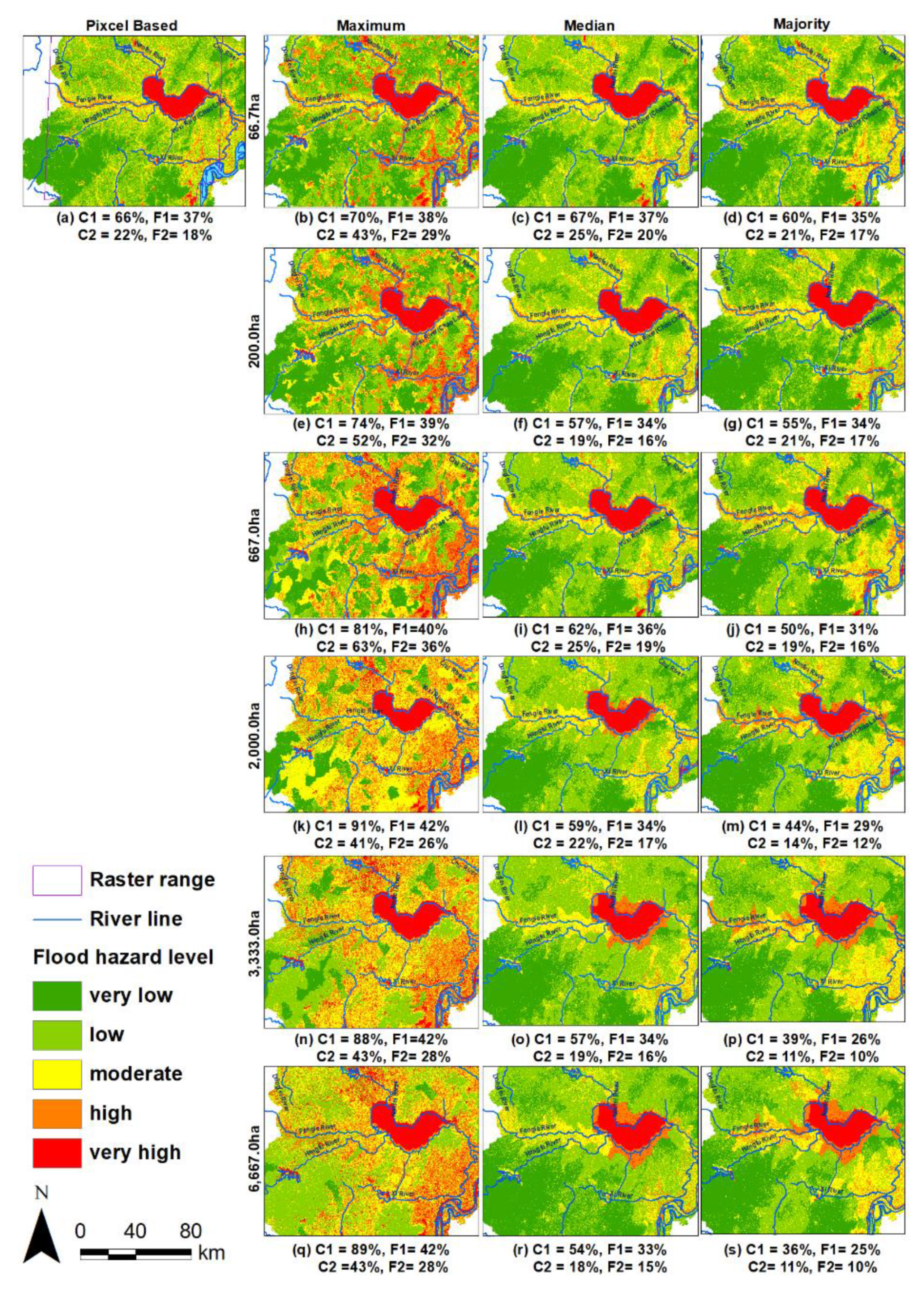
Figure 10.
Flood risk levels from pixel-based AHP (a) and sub-watershed based AHP using D8-derived sub-watershed to constrain converging related indicators, such as Elevation, Slope and Distance from Streams (b–s).
Figure 10.
Flood risk levels from pixel-based AHP (a) and sub-watershed based AHP using D8-derived sub-watershed to constrain converging related indicators, such as Elevation, Slope and Distance from Streams (b–s).
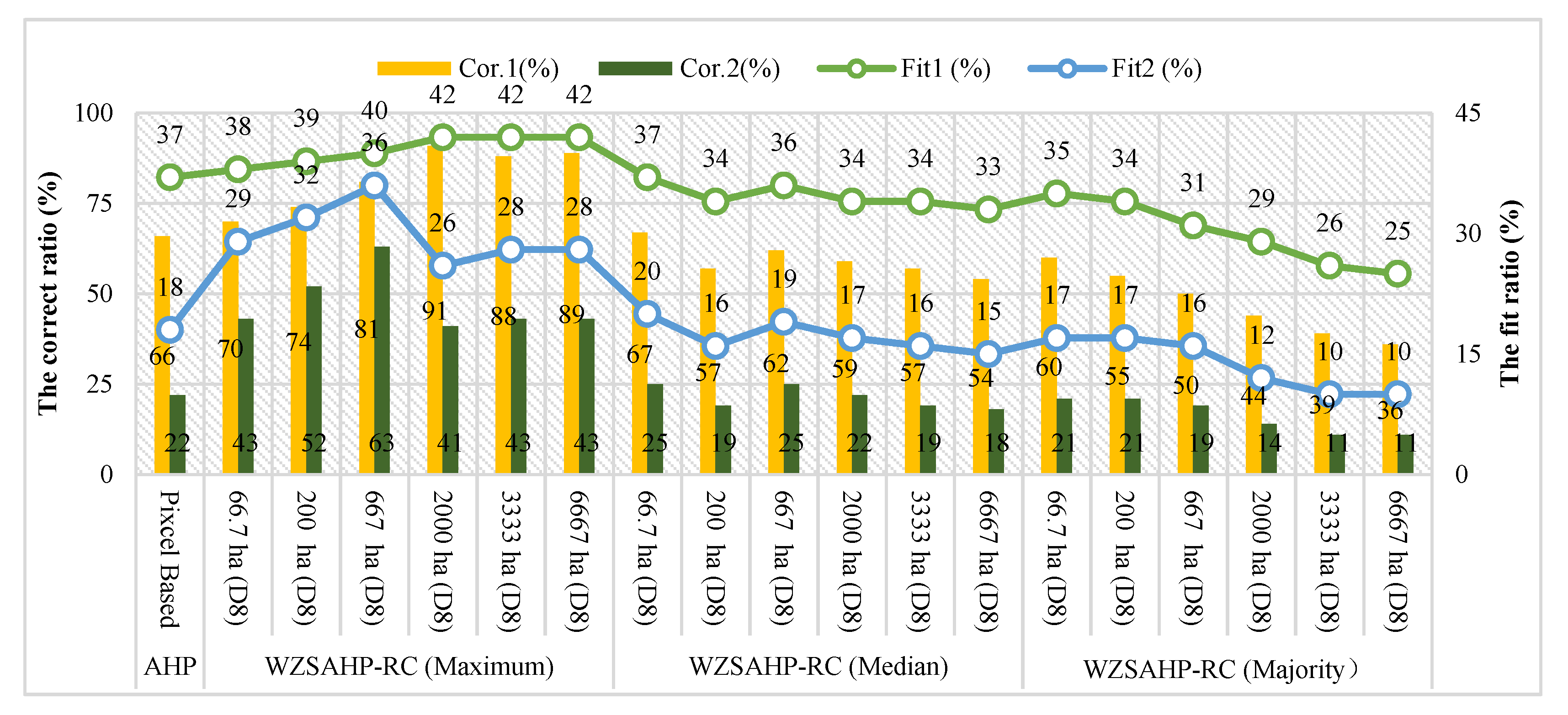
Figure 11.
The correct ratio and fit ratio values of pixel-based AHP and the WZSAHP-RC using D8 derived sub-watershed to constrain converging related indicators.
Figure 11.
The correct ratio and fit ratio values of pixel-based AHP and the WZSAHP-RC using D8 derived sub-watershed to constrain converging related indicators.
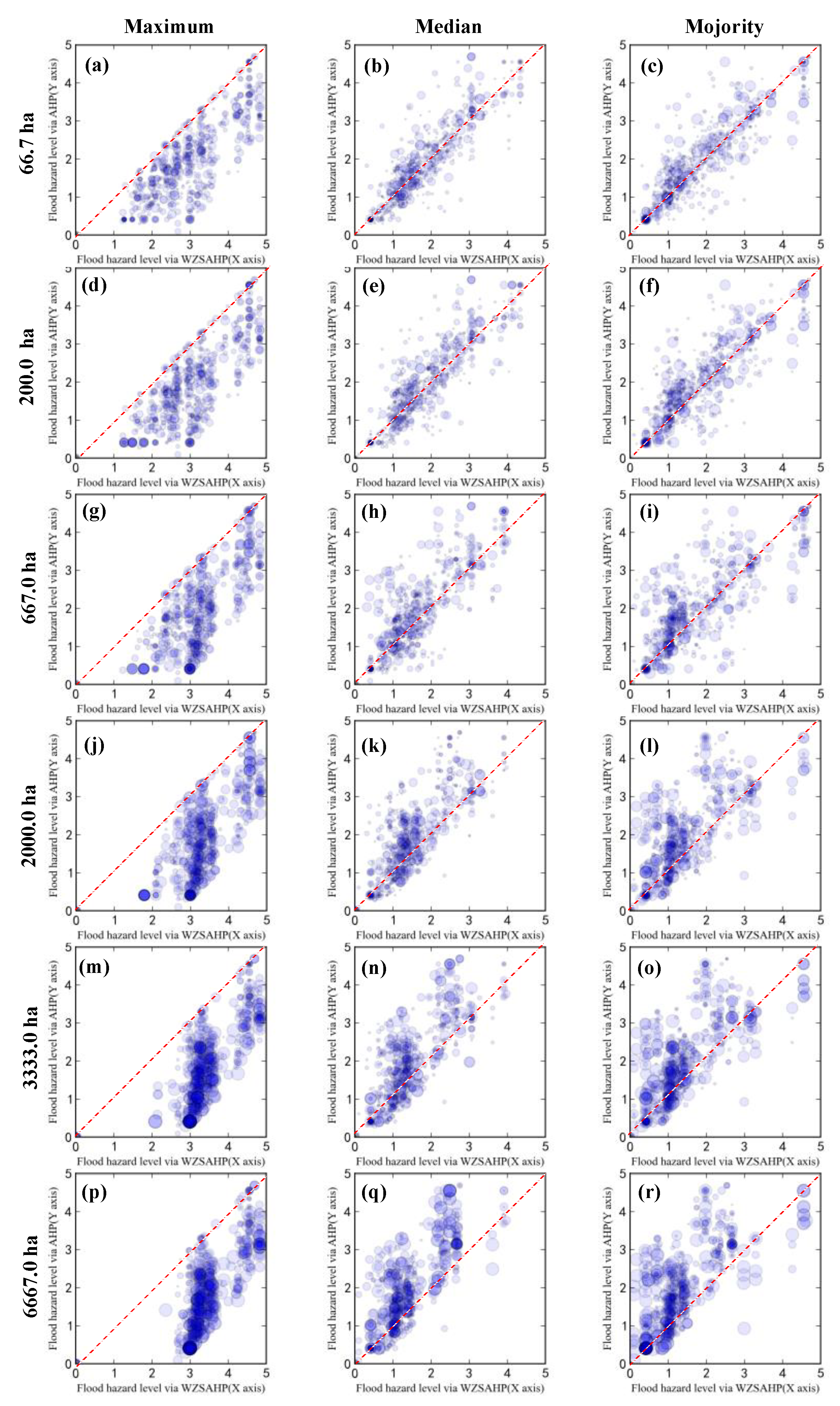
Figure 12.
Scatter diagrams of flood hazard indexes distribution sampled by WZSAHP-RC via D8 delimitated sub-watershed a basic unit (WZSAHP-RC-D8) and AHP methods. The subfigures (a–r) used the flood hazard index derived by WZSAHP-RC-D8 as X-axis and using flood hazard index derived by AHP as Y-axis.
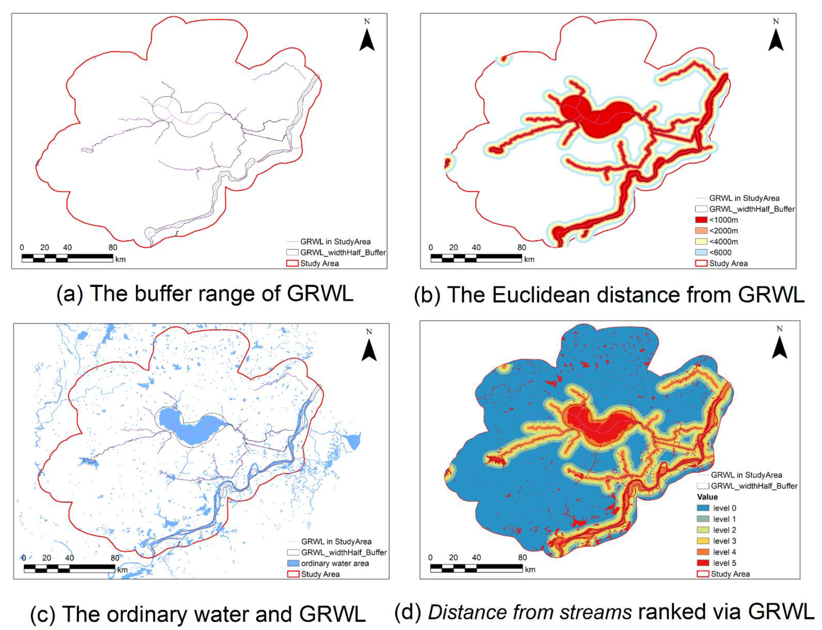
Figure 13.
The GRWL distribution and the GRWL-based Distance from streams indicator in the study area. Figure (a) was the GRWL vectors and corresponding buffer results basing the attribute value of the width, figure (b) was the Euclidean distance from the GRWL buffer border, and figure (c) was the ordinary water bodies overlying the GRWL buffer layer and the ranked “Distance from streams” indicator in figure (d) was derived by GRWL and normal water range.
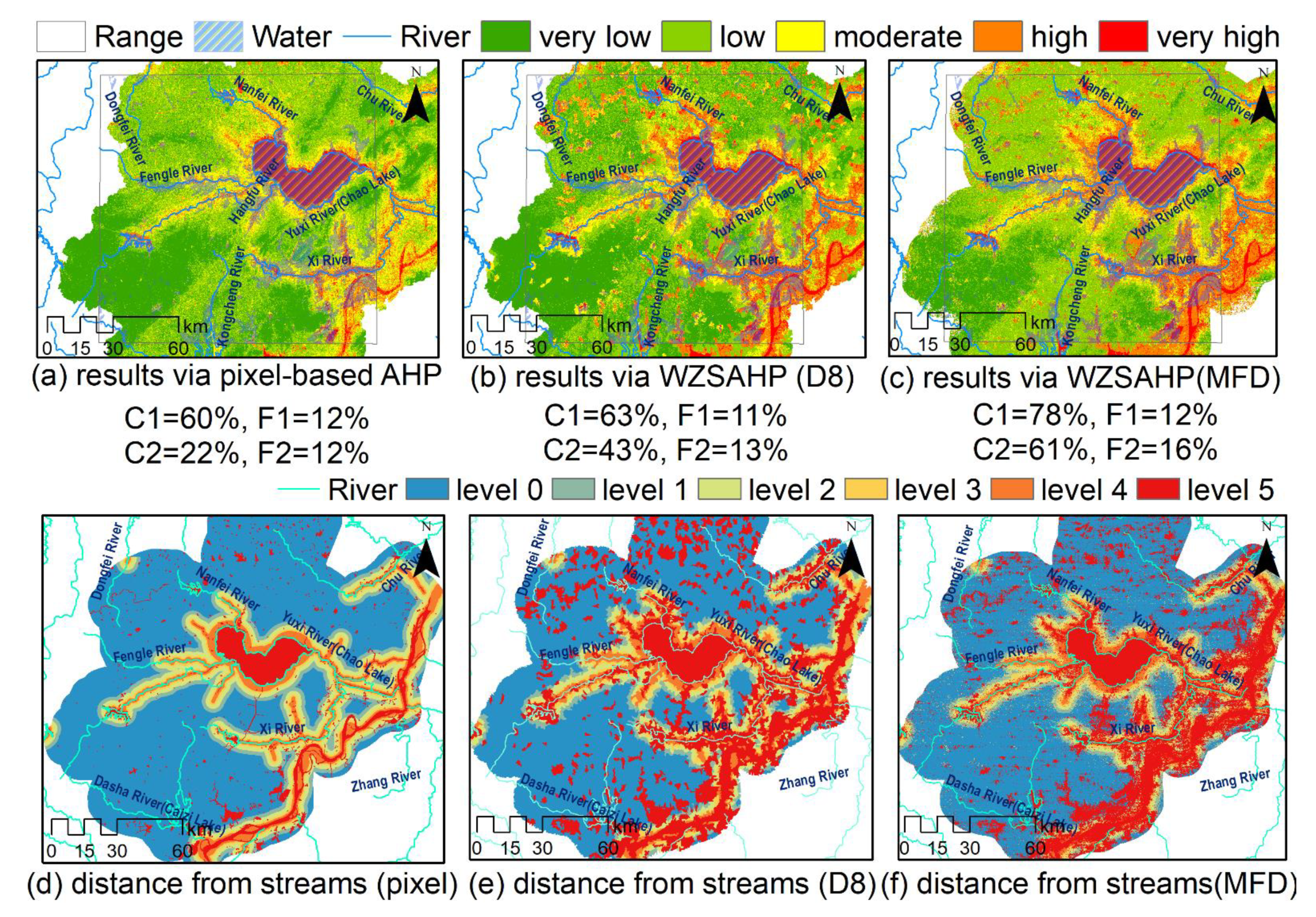
Figure 14.
The flood hazard distribution derived by pixel-based AHP, the WZSAHP-RC using D8-derived and MFD to classify sub-watersheds as basic units. (a–c) were the flood hazard distribution basing pixel-based AHP, WZSAHP via D8-derived sub-watershed, and WZSAHP via MFD derived sub-watershed, respectively. (d–f) were the GRWL derived distance from streams distribution using pixel-based AHP, WZSAHP via D8-derived sub-watershed, and WZSAHP via MFD derived sub-watershed, respectively.
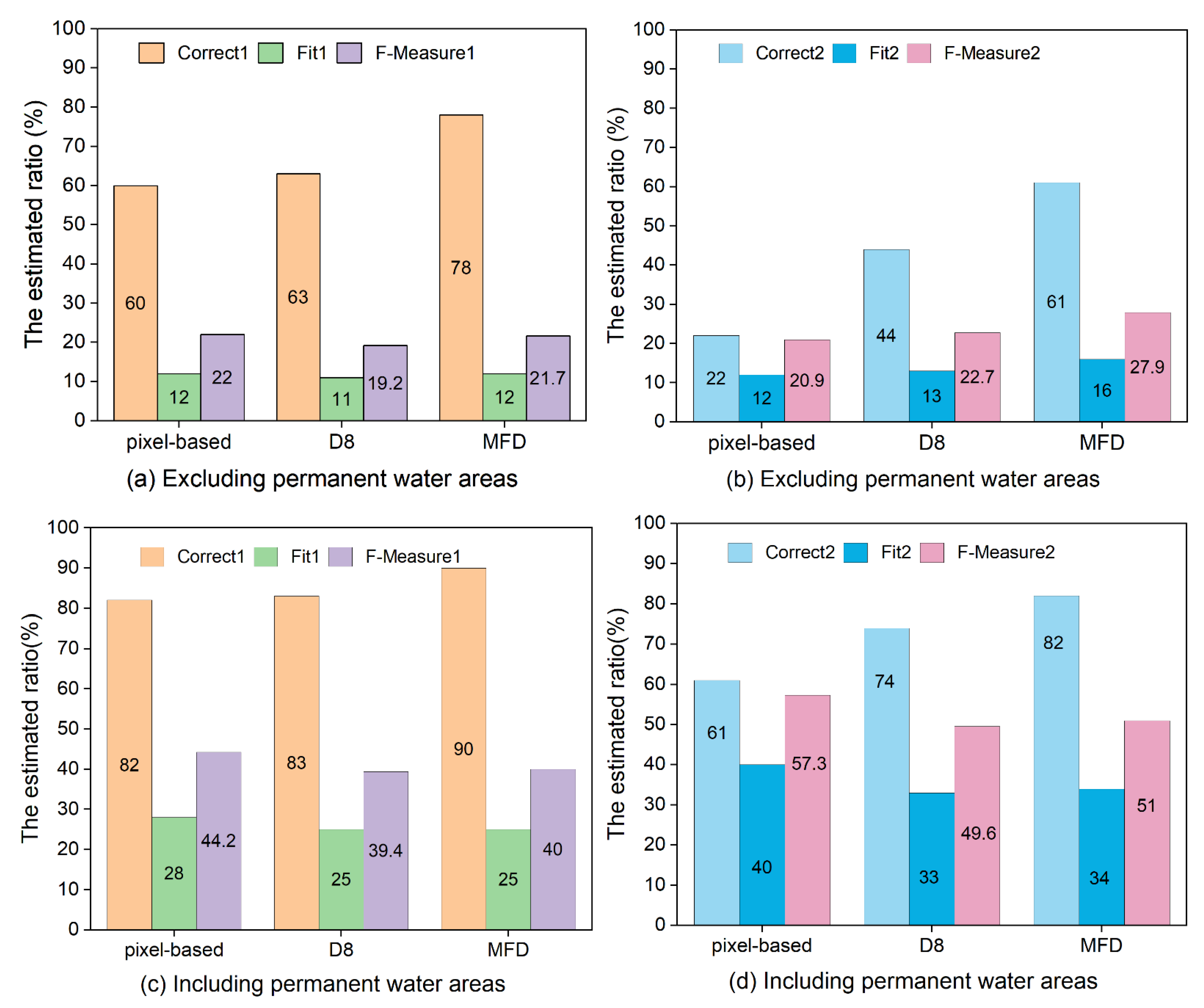
Figure 15.
The correct ratio, fit ratio and F-measure basing the validation dataset excluding permanent water areas and including permanent water areas. (a,b) were the validation ratio using floodwater areas excluding permanent water areas. In contrast, (c,d) was the validation ratio using all water areas on flood days.
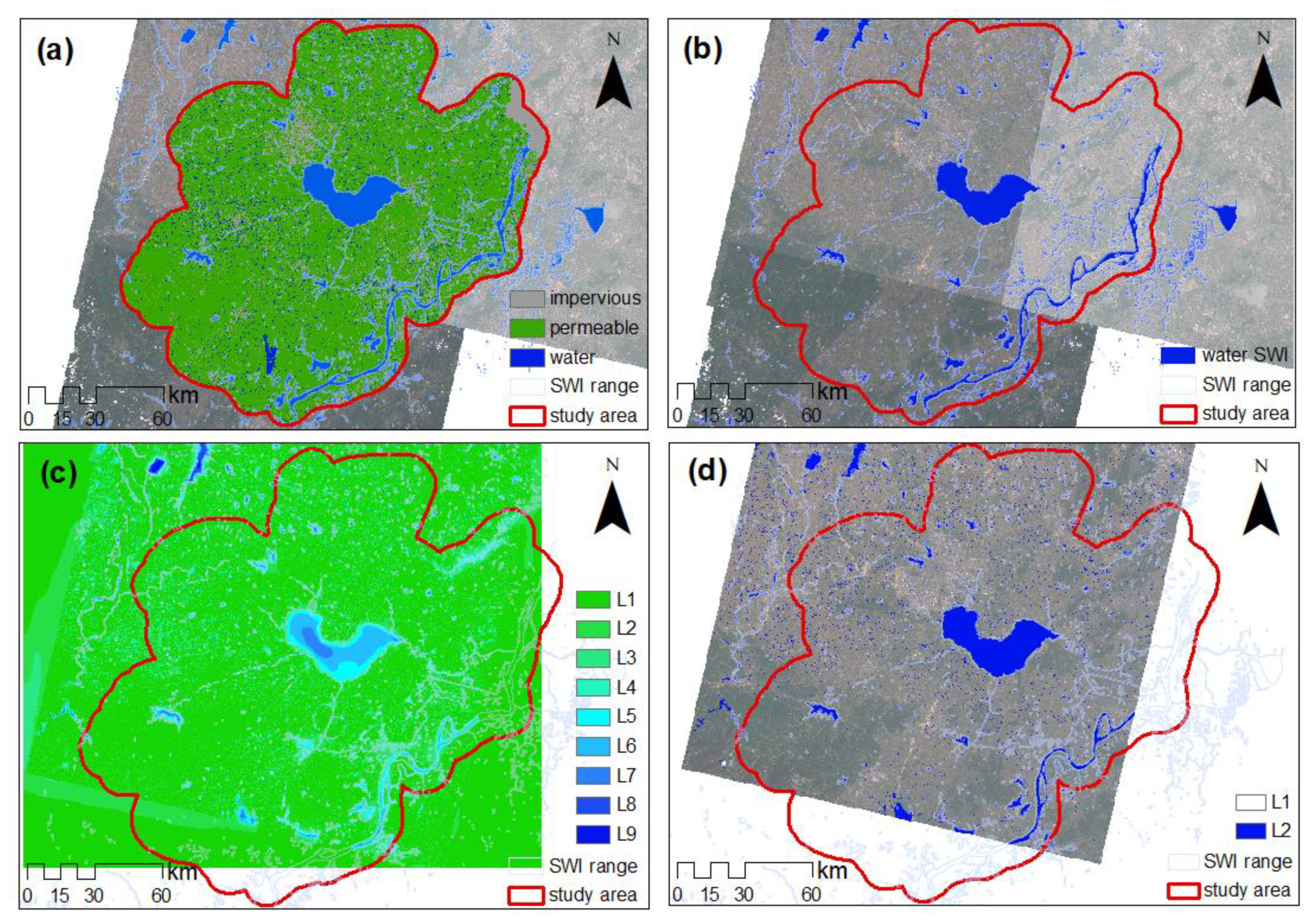
Figure 16.
The normal water range extract by the proposed SWI and the RivaMap. (a) was the range of water bodies extracted by SWI overlay the distribution of the impervious surface production, (b) was the water body and range areas of SWI, and (c,d) were the distributions of the multiscale singularity index of RivaMap classified by nature break method as nine types and two types.
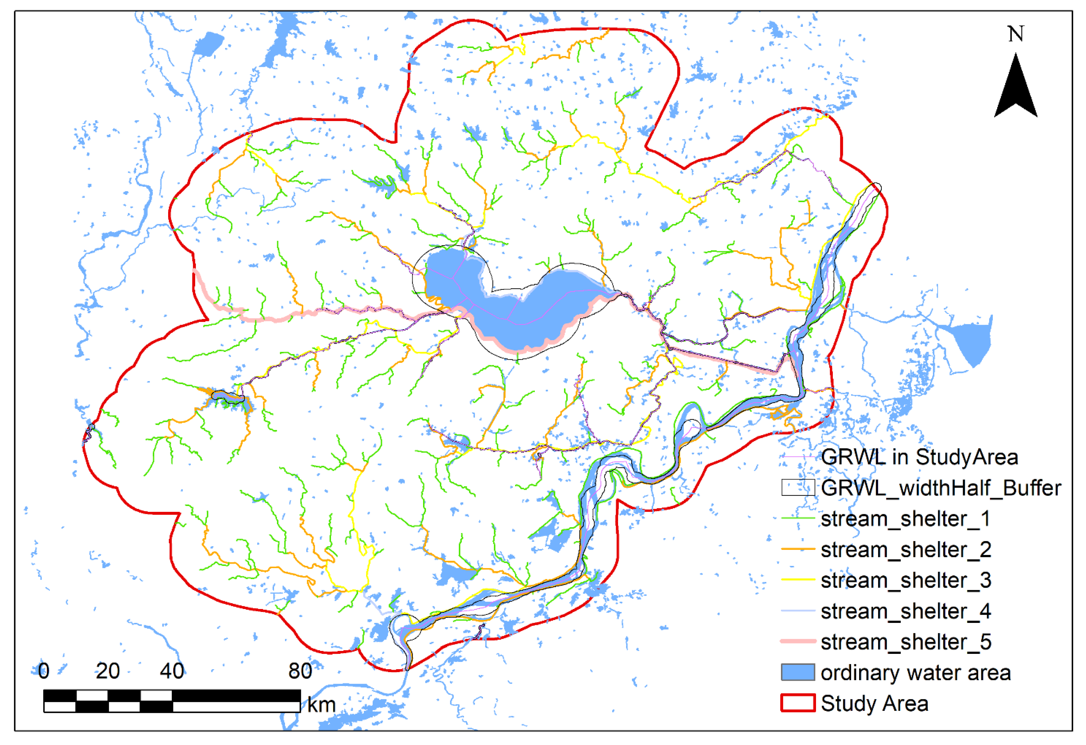
Figure 17.
The distribution of GRWL in the study areas, overlaid by the digital streams derived by DEM, and the common water area in the study area.
Figure 17.
The distribution of GRWL in the study areas, overlaid by the digital streams derived by DEM, and the common water area in the study area.
Table 1.
The main data materials used in this study.
Table 1.
The main data materials used in this study.
| Data Sources | Used Data | Detailed Information |
|---|
| Geographic information (1:1 million) | District | The county and town level districts were used. Hydrological layers were utilized to constrain DEM. They were downloaded from the China Science and Technology resources sharing network, Available online: http://www.geodata.cn/data/datadetails.html?dataguid=113730965998632 (accessed on 20 July 2020). |
| River and lake |
| ASTER GDEM V2 (30 m) | DEM | The DEM divides watersheds and classifies the slope and elevation indicators. The DEM was downloaded from Available online: http://www.gscloud.cn (accessed on 20 July 2020). |
| China’s impermeable surface product (2 m) | Land-use type | Following [21], the water, vegetation, soil, building and road layers were used to classify land use and hydrological indicators. China’s impermeable surface production (2 m) dataset is not published on the website. In this study, the involving land use type vector collected from this product can be downloaded according to the detailed description in the Supplementary Material section. |
| Hydrological characteristics |
| Images for extracting flooding areas | Water bodies | The Landsat 8 OLI on 20 July 2020 and GF-3 on 24 July 2020 were used to extract flooding areas. The Landsat 8 OLI was downloaded from Available online: https://www.usgs.gov (accessed on 20 July 2020). The GaoFen center of Hubei province supports the GF-3 data, and it also can download from the China Science and Technology resources sharing network: Available online: http://39.106.90.21/datashare/newsatelliteset2.html (accessed on 20 July 2020). |
| Flooding information in Baidu News | Flooding and dam breaks by towns | Baidu News, as a validation source, was searched from Available online: http://news.baidu.com (accessed on 20 July 2020). |
Table 2.
The judgment matrix of criteria. C1 = Slope, C2 = Elevation, C3 = Distance from streams, C4 = Hydro-lithological formations, C5 = Land use type.
Table 2.
The judgment matrix of criteria. C1 = Slope, C2 = Elevation, C3 = Distance from streams, C4 = Hydro-lithological formations, C5 = Land use type.
| Flood Hazard Potential | C1 | C2 | C3 | C4 | C5 |
|---|
| C1 | 1 | 4 | 1/2 | 3 | 1/2 |
| C2 | 1/4 | 1 | 1/3 | 1/2 | 1/4 |
| C3 | 2 | 3 | 1 | 3 | 1 |
| C4 | 1/3 | 2 | 1/3 | 1 | 1/3 |
| C5 | 2 | 4 | 1 | 3 | 1 |
Table 3.
The classes and rating of factors in flood hazard estimation.
Table 3.
The classes and rating of factors in flood hazard estimation.
| Factors | Classes | Rating | Factors | Classes | Rating |
| Slope (°) | 0 | 5 | Land use types | Water | 5 |
| 0–2 | 4 | Road | 4 |
| 2–6 | 3 | Building | 3 |
| 6–12 | 2 | Soil | 2 |
| 12–20 | 1 | Vegetation | 1 |
| >20 | 0 | | |
| Elevation (m) | −204–12 | 5 | Hydro lithological formations | Water | 4 |
| 12–23 | 4 | Impermeable surface | 3 |
| 23–46 | 3 | Pervious surface | 1 |
| 46–152 | 2 | | |
| >152 | 1 | | |
| Factors | Classes | Rating |
| Distance from streams (m) | Rivers, lakes and reservoirs | 5 |
| Level 1 | Level 2 | Level 3 | Level 4 | Level 5 | |
| | | | | 0–1000 | 4 |
| | | 0–500 | 0–1000 | 1000–2000 | 3 |
| | 0–500 | 500–1000 | 1000–2000 | 2000–4000 | 2 |
| 0–500 | 500–1000 | 1000–1500 | 2000–3000 | 4000–6000 | 1 |
| >500 | >1000 | >1500 | >3000 | >6000 | 0 |
Table 4.
Area threshold used in delimitation watersheds via D8 algorithm.
Table 4.
Area threshold used in delimitation watersheds via D8 algorithm.
| Basic | Area Unit | (1) | (2) | (3) | (4) | (5) | (6) |
|---|
| 667 | ha | 66.7 | | 667.0 | | 3333.0 | 6667.0 |
| mu | ~10,000 | | ~100,000 | | ~500,000 | ~1,000,000 |
| 200 | ha | | 200.0 | | 2000.0 | | |
| mu | | ~30,000 | | ~300,000 | | |
Table 5.
The classes and rating of factors in flood hazard estimation.
Table 5.
The classes and rating of factors in flood hazard estimation.
| | Validation 1 | Validation 2 |
|---|
| Positive Group: “Very High”, “High”, “Moderate” | Negative Group: “Very Low”, “Low” | Positive Group: “Very High”, “High” | Negative Group: “Very Low”, “Low”, “Moderate” |
|---|
| flooded area | TP | FN | TP | FN |
| dry area | FP | TN | FP | TN |
| normal water | / | / | / | / |
Table 6.
The comparison matrix and correct ratio, fit ratio, F1-score of flood hazard and flooded areas distribution.
Table 6.
The comparison matrix and correct ratio, fit ratio, F1-score of flood hazard and flooded areas distribution.
| Items | Validation 1 | Validation 2 |
|---|
| Positive Group (P): “Very High”, “High”, “Moderate” | Negative Group (N): “Very Low”, “Low” | Positive Group (P): “Very High”, “High” | Negative Group (n): “Very Low”, “Low”, “Moderate” |
|---|
| Flooded area (T) | 842,963 | 131,230 | 583,933 | 390,260 |
| Dry area (F) | 1,004,991 | 302,577 | 673,359 | 634,209 |
| Correct ratio (%) | 87 | 60 |
| Fit ratio (%) | 43 | 35 |
| F1-Score | 0.597 | 0.523 |
Table 7.
The correct ratio, fit ratio and F1-score were calculated by the pixel-based AHP method and the proposed sub-watershed-based WZSAHP-RC method.
Table 7.
The correct ratio, fit ratio and F1-score were calculated by the pixel-based AHP method and the proposed sub-watershed-based WZSAHP-RC method.
| Adopted Method | Base Unit | Validation 1:
Positive Group (P): “Very High”, “High”, “Moderate”; Negative Group (N): “Very Low”, “Low” | Validation 2:
Positive Group (P): “Very High”, “High”; Negative Group (N): “Very Low”, “low”, “Moderate” |
|---|
| Cor.1 (%) | Fit1 (%) | F1-Score | Cor.2 (%) | Fit2 (%) | F1-Score |
|---|
| AHP | Pixel | 67 | 37 | 0.542 | 22 | 18 | 0.298 |
| WZSAHP-RC | Sub-watershed | 83 | 43 | 0.597 | 60 | 35 | 0.523 |
| Increasing (%) | / | 16 | 6 | / | 34 | 17 | / |


