Review

A Review on the Possibilities and Challenges of Today’s Soil and Soil Surface Assessment Techniques in the Context of Process-Based Soil Erosion Models

1
Department of Physical Geography, Friedrich-Schiller University Jena, 07743 Jena, Germany
2
District Administration Siegen-Wittgenstein, Administrative Department for Climate and Sustainable Mobility, 57072 Siegen, Germany
3
Thuringian State Institute of Agriculture, 07743 Jena, Germany
4
Institute of Photogrammetry and Remote Sensing, Technical University Dresden, 01069 Dresden, Germany
5
Institute of Drilling Engineering and Fluid Mining, Flow and Transport Modelling in the Geosphere, TU Bergakademie Freiberg, 09599 Freiberg, Germany
6
Department Ecology and Environment, IPROconsult GmbH, 01069 Dresden, Germany
7
Institute of Geoecology, Landscape Ecology and Environmental Systems Analysis, TU Braunschweig, 38106 Braunschweig, Germany
*
Author to whom correspondence should be addressed.
Remote Sens. 2022, 14(10), 2468; https://0-doi-org.brum.beds.ac.uk/10.3390/rs14102468
Submission received: 4 April 2022 / Revised: 12 May 2022 / Accepted: 19 May 2022 / Published: 20 May 2022
(This article belongs to the Special Issue Quantifying Landscape Evolution and Erosion by Remote Sensing)

Abstract

:
To investigate relevant processes as well as to predict the possible impact of soil erosion, many soil erosion modelling tools have been developed. The most productive development of process-based models took place at the end of the 20th century. Since then, the methods available to observe and measure soil erosion features as well as methods to inter- and extrapolate such data have undergone rapid development, e.g., photogrammetry, light detection and ranging (LiDAR) and sediment tracing are now readily available methods, which can be applied by a broader community with lower effort. This review takes 13 process-based soil erosion models and different assessment techniques into account. It shows where and how such methods were already implemented in soil erosion modelling approaches. Several areas were found in which the models miss the capability to fully implement the information, which can be drawn from the now-available observation and data preparation methods. So far, most process-based models are not capable of implementing cross-scale erosional processes and can only in parts profit from the available resolution on a temporal and spatial scale. We conclude that the models’ process description, adaptability to scale, parameterization, and calibration need further development. The main challenge is to enhance the models, so they are able to simulate soil erosion processes as complex as they need to be. Thanks to the progress made in data acquisition techniques, achieving this aim is closer than ever, if models are able to reap the benefit.

Graphical Abstract

1. Introduction

Soil, a natural resource with essential functions to the ecosystem, has experienced extensive degradation over the past decades [1,2]. Soil erosion can lead to soil loss and eventually to the exposure of the underlying bedrock [3]. It represents a decisive process for degrading agricultural land and thus crop yield on a global scale [4,5,6]. Climate change causes an increase in frequency of extreme weather events and therefore leads to spatially differentiated changes in extent, intensity and frequency of soil erosion [7,8,9,10]. Alongside the direct impact of climate change, it also triggers indirect drivers of soil erosion, such as crop management or land use changes [9,10], varying greatly with the region [11,12,13].
While soil erosion on arable land is usually higher than on non-arable land [14], the degree of erosion largely depends on land management practices. Therefore, adapted land management is an important step towards the sustainable use of soils [15]. The protection and conservation of soils has become a major social challenge worldwide and represents an important field of research [16]. In order to support soil protection efforts and recovery strategies, it is necessary to accurately assess erosion rates and information on erosion, transport and sedimentation processes [2,17].
Research on this topic started in the early 20th century, with the first modelling approaches in the 1940s by Zingg [17] quoted in [18] and the development of an empirical soil erosion model, the so-called universal soil-loss equation (USLE), by Wischmeier and Smith [18]. With the improvement of computing power, data availability and for a better process understanding, such empirical models were followed by process-based soil erosion models. These have certain advantages over the empirical models, for example they are supposed to be easily transferable to other sites and scales and are able to view soil erosion processes based on physical principals [19,20].
Most process-based soil erosion models were developed at the end of the 20th century (Figure 1). These models did not have access to the possibilities and input data of today. While increasing computing power is constantly pushing the limits of data collection, processing and modelling, new opportunities in assessing and using soil data and in understanding soil erosion processes become available. Continuous development and improvement of measurement techniques lead to spatially and temporally highly resolved information on different scales [21].
Most process-based models demand some kind of measured soil data (e.g., texture, water retention function, hydraulic conductivity, aggregate stability), which are mostly not available in a high resolution. However, recent data assessment techniques, especially regarding remote sensing methods, offer new information, and by that the potential for model development as well as model ensemble strategies. Furthermore, we consider cross-process as well as cross-scale understanding of soil erosion on different spatial and temporal scales as a valuable step towards improved process-based soil erosion modelling. To gain a more holistic understanding and achieve an impact reduction by applying adapted management strategies, models need to integrate the current understanding of soil erosion processes from splash to gully erosion [8,26]. For future model development, we find it crucial to determine in what way the present assessment techniques can contribute to the improvement of process-based soil erosion models. The models show difficulties in describing different processes, e.g., connectivity, soil compaction or rill initiation. This results in a need for observation that could be specifically covered by the new and improved methods.
Altogether this raises the question of which of the formerly limiting factors, both in terms of model capabilities and data availability may have become obsolete. Can modernised measurement techniques, recent data on soil and soil erosion, a new range on resolutions and the latest achievements regarding computing power help to effectively develop these models? To address this question, the work is structured considering the following aspects:
  • State-of-the-art
    • What are the strengths and weaknesses of process-based soil erosion models?
    • What are the opportunities and limitations offered by the present data assessment techniques regarding the model parameterization and process description?
  • Limitations and opportunities offered by assessment techniques regarding process-based soil erosion models
    • Can today’s data assessment overcome shortcomings and improve existing models?
    • Can soil erosion process descriptions be delineated from modern erosion measurement techniques and integrated into these models?
    • Can data help to produce, parameterize and validate existing process-based soil erosion models or is there a need for a new modelling approach altogether?
Many reviews regarding empirical and process-based soil erosion models already exist. Borrelli et al. [26] just recently gave a comprehensive overview of the literature regarding soil erosion prediction models. Reviewing 1679 studies published between 1994 and 2017, they provide a state-of-the-art insight on soil erosion modelling on a global scale. According to their research, a huge challenge in soil erosion management is still the lack of knowledge in large parts of the world. To help overcome this research gap we specialised our research, not on the modelling alone, as has been done many times before (e.g., [10,21,23,25]), but in combination with assessment techniques available today. Combining these aspects, we aim to identify where available data can help improve and further develop process-based soil erosion models. We therefore offer an overview of the potentials and shortcomings of soil, soil erosion and soil surface assessment techniques by examining process-based soil erosion models and their possibilities for implementing data from new and improved measurement techniques. Along this interface, based on today’s possibilities of data generation and processing, this work aims to identify the factors relevant to overcoming the limitations of process-based soil erosion modelling, and to its improvement.

2. Soil Erosion Assessment

Today, a large number of soil erosion models exist, and a wide range of methods for measuring soil erosion processes by water have been developed. In the following we present a selection of process-based soil erosion models. Their possibilities and limitations, as well as their scale and process understanding, have been taken into account. Subsequently, we provide a selective overview of different soil erosion assessment techniques we see as relevant in either providing a new cross-scale process understanding or offering valuable and improved data for model parameterization.

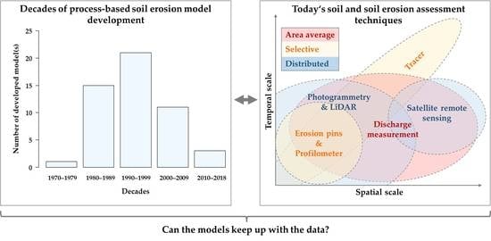
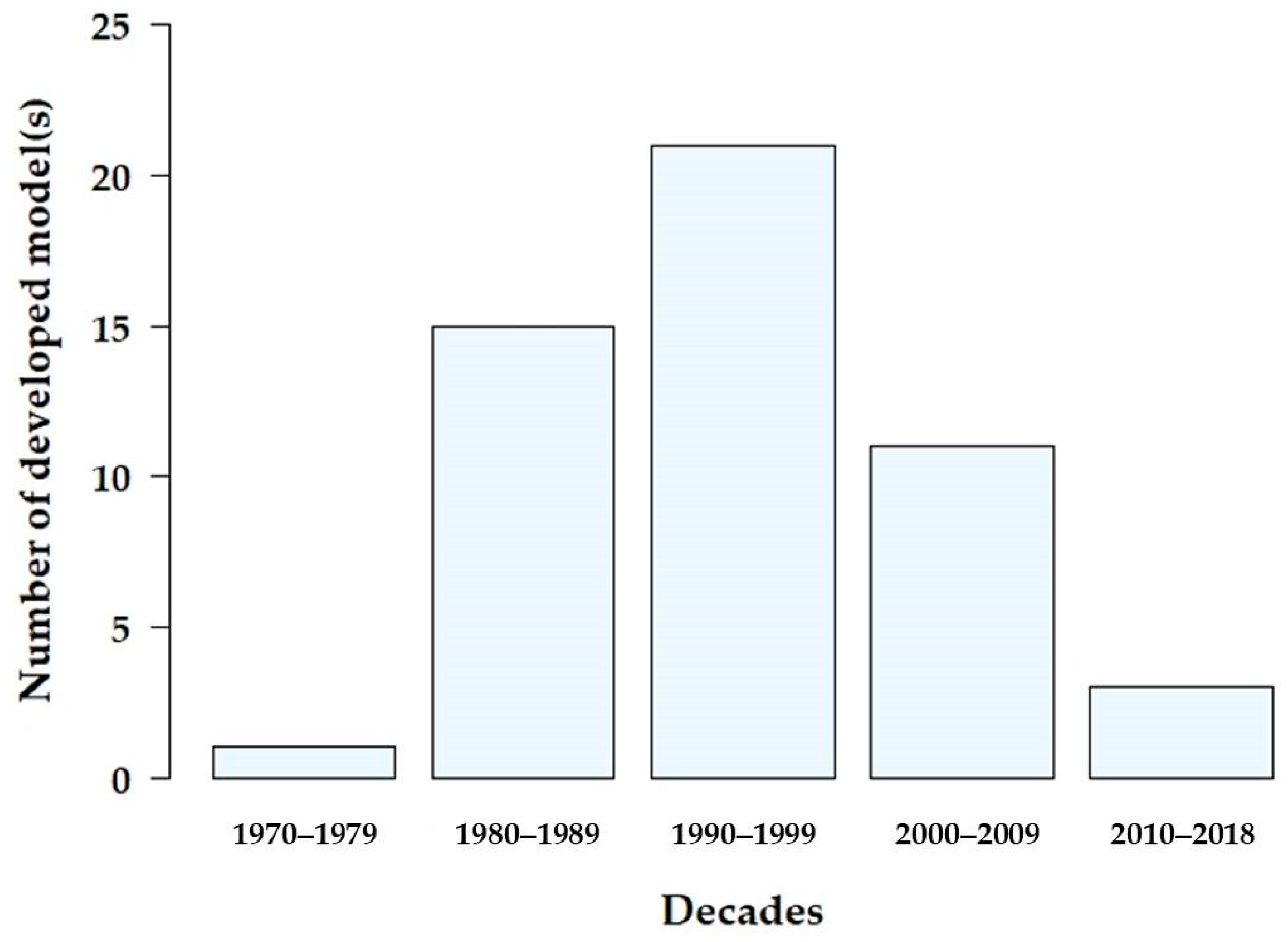
2.1. Process-Based Soil Erosion Models

Models are simplifications of reality and can, by definition, never fully represent the processes of the real world. Because these models can only come close to reality, researchers are looking for a balance between modelling and reality. Depending on their area of speciality, models feature different advantages and limitations. With improving knowledge, computing power and observational technologies, these limitations are constantly shifting towards models that are more realistic while also showing limits regarding reality. Where to exactly draw this line poses an almost philosophical question, answerable only by each individual model. In comparison to empirical models, process-based soil erosion models are more demanding regarding their input data, computing requirement and calibration necessity, and in general are less user-friendly. However, due to physically-based descriptions of soil erosion and sediment transport, the models offer an understanding and reproducibility of the occurring processes [23]. Such models allow for an isolated consideration of individual components of soil erosion processes as well as a better understanding of the relationship between cause and impact within soil erosion research [19]. While these models are process-oriented, they still contain empirical parts based on laboratory and site-specific field experiments. Even though they can be extrapolated to other scales, this aspect must still be treated with care [27].
In recent years, several authors have reviewed soil erosion models, taking different perspectives into account [10,21,22,23,25,28,29]. They offer a broad overview of available process-based soil erosion models, along with their strengths and weaknesses. As models are conceptualised for different purposes as well as for different spatial and temporal scales [24], they vary widely regarding their complexity, data demand, temporal and spatial representation of process mapping, input parameters and outputs [21]. Jetten and Favis-Mortlock [28] highlight the challenge that different models are developed for special spatial and temporal scales and therefore mostly incorporate a scale-specific process mapping. Restrictions such as these are often accompanied by the practical aspect of data availability [21]. Models consequently often assume continuous temporal soil and surface input parameters, which can lead to wrong process description [28]. The prediction quality of a model is heavily influenced by its input data and its parameterization. Therefore appropriate data collection from multiple sources, accurate model parameterization and temporal and spatial high-resolution input data are important aspects of model improvement [21,30]. Parsons [27] sees the simulation capability of the models constrained by the underlying process description and consequently by our understanding of soil erosion processes. Thus, the potential for model improvement can be the use of revised process descriptions such as rill-interrill interaction [22] or gully erosion [23].
In Table 1 we have compiled, a selection of process-based soil erosion models, derived from Aksoy and Kavvas [22], Karydas et al. [24], Hajigholizadeh et al. [23], Merritt et al. [25] and Pandey et al. [21]. We further constricted the selection to those more frequently used models since 2000 (more than 10 publications). In this way, we made sure to capture the most relevant models without having a table that is oversized for the purpose of this manuscript. The table is structured according to the different processes considered by soil erosion modelling. Because a holistic listing of model limitations cannot be implemented and would go beyond the scope of such a table, we decided to list the possibilities of the models instead. Conversely, their limits can be derived from their strengths, which are based mainly on equations and coefficients. Figure 2 provides a historical classification of these models. While, as presented in Figure 1, many models were developed before the end of the 20th century, research regarding those existing models has since increased. Based on Google Scholar searches, looking for research titles including the model’s name and “erosion”, Figure 2 gives an overview of the consistent, increasing or decreasing usage of the different process-based soil erosion models over the past fewndecades. Google Scholar was chosen because of its free availability, transparency, reproducibility and the broad spectrum of sources taken into account. Because only manuscripts mentioning the model and erosion in the title have been considered, this analysis only gives an impression and cannot claim to be exhaustive. The EUROSEM model shows a decrease of usage, while publications on the models EROSION 3D and especially WEPP have increased significantly. A constant application since its development can be found by the model LISEM.
Table 1 highlights in which areas, in regard to their process mapping, process-based soil erosion models show strengths and weaknesses. Non-addressed processes can especially be found in the fields of particle detachment within rills, particle size distribution, deposition, and flow routing. The last column of the table, flow routing, reveals the greatest gaps and is, even when considered by models, mostly treated only statically. While RillGrow presents an exception, most approaches have difficulties in adapting the relief during the modelling process. Of these models RillGrow alone is able to depict rills dynamically. Even though it offers a self-organizing system, enabling feedback loops on the microtopography, it also neglects important aspects such as infiltration and deposition. Backwater, diffusion and dynamic distribution of shallow water by water surface elevation can only be solved by the more complicated equations, such as the Saint Venant equation, which results in even more complex models. However, as these models are all simplifications of reality, the all-achieving model cannot exist, which results in a constantly rising and gradually confusing number of models with a range of different strengths and weaknesses. Presenting the limiting factors of a selection of process-based soil erosion models might indicate starting points for necessary model improvement. In this context, we investigate which processes can be observed on a new temporal and spatial scale and where these methods can be used to further develop process-based soil erosion models.

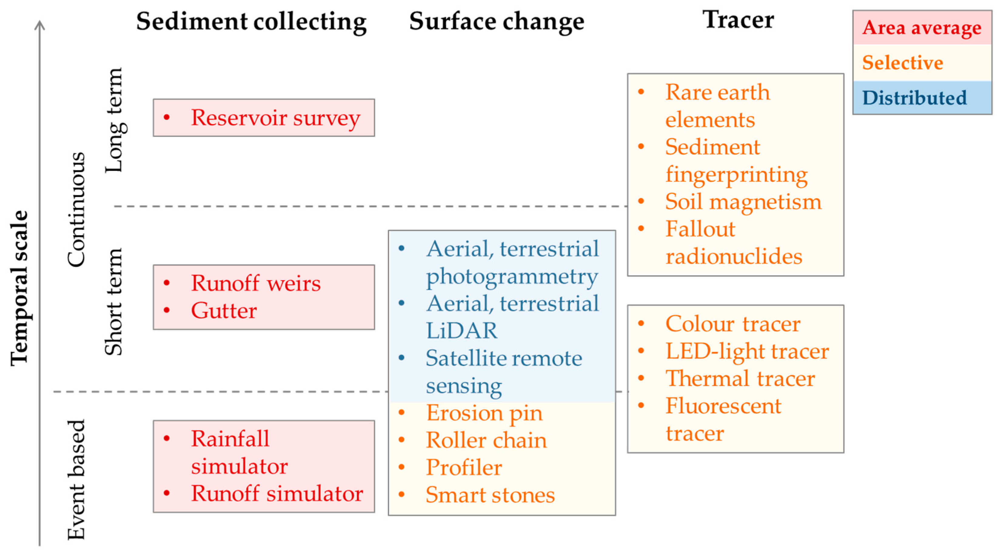
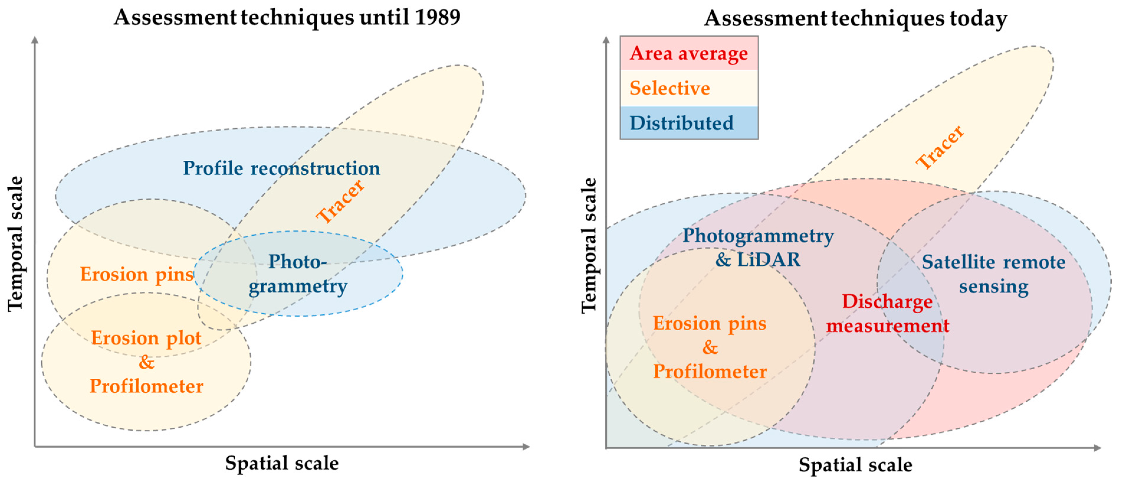
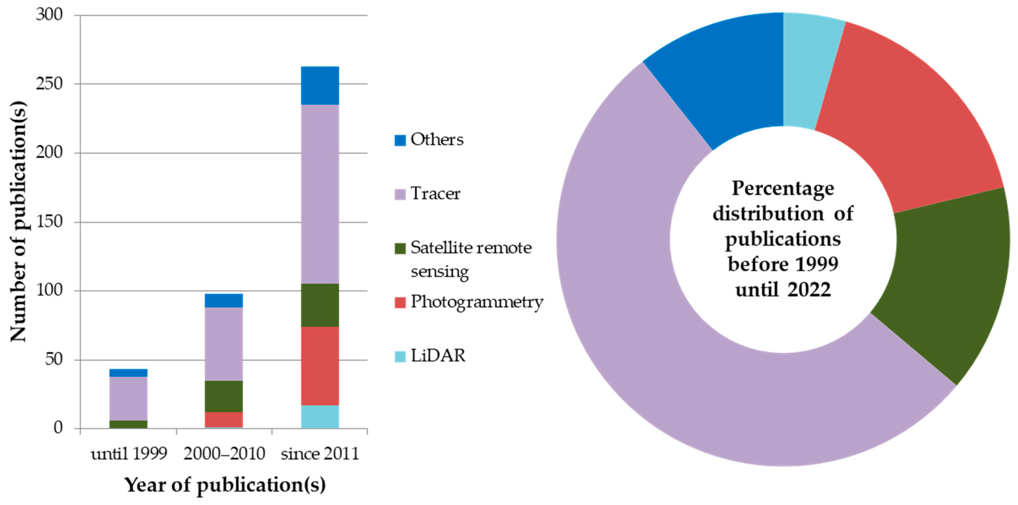
2.2. Techniques on Soil Erosion Measurement

Measurement techniques to assess soil properties, soil surface and soil erosion are constantly advancing in terms of their spatial and temporal resolution [71]. In reviewing those, a holistic approach hardly seems achievable; therefore, most researchers focus on comparing a selection of similar technological approaches, such as, e.g., Padarian et al. [72], concentrating on different machine learning (ML) approaches, or Castillo et al. [73], comparing LiDAR, laser profilometre, a total station and 3D photo-reconstruction in the context of gully erosion. Others give a broad overview of different assessment areas but do not go into detail regarding the individual techniques, such as Parsons [27], summarising information on plot studies, monitoring and measurement techniques and modelling approaches. For more quantitative and precise approaches and to gain an improved understanding of processes and connectivity, both Li et al. [71] and Rodrigo-Comino [74] suggest applying the methods combined on different temporal and spatial scales. Regarding process-based soil erosion models, such new assessment techniques and the resulting data are especially interesting, considering the following two factors:
  • Recently improved methods offer new data, which can be used to feed process-based soil erosion models and offer spatial and temporal distributed model parameterization.
  • Models are based on specific equations and therefore focus on certain processes and certain scales. Of interest are methods which offer new temporal and spatial cross-scale knowledge on soil erosion processes and their distribution. Such data can be used to validate available process understanding or even integrate new process understanding into models.
The choices of method discussed in this review were selected and structured on the basis of these two categories and do not claim to be exhaustive. For certain, many more techniques have been developed and improved, offering new information and data valuable for process-based soil erosion models. A holistic view of all such methods would go beyond the scope of this paper. This work presents different methods which enable either new and improved data availability or a new and improved process understanding. Figure 3 offers a selection of different soil and soil erosion assessment techniques, structured by their type of assessment, their temporal scale and their output. It distinguishes methods for assessing data for a whole area at one outlet (area average), point source data (selective) and those assessing exhaustive data for the research area (distributed). Summarised in categories, Figure 4 provides an overview of the development of soil and soil erosion techniques between 1989 and today. It also further visualises the categories structured by their temporal scale of application on a spatial scale. The same colouring as in Figure 3 gives an insight into the type of output data to be expected. Figure 4 emphasises what can also be found after a structured literature analysis with the Google Scholar search engine visualised in Figure 5. Photogrammetric and tracing techniques show a huge increase in research. The literature analysis has shown that within the broad category of tracing, fallout radionuclides and sediment fingerprinting make up the largest part, and in the category of photogrammetry, Structure from Motion (SfM) proves to be researched the most.
All three figures (Figure 3, Figure 4 and Figure 5) offer only estimations and do not claim to be exhaustive. Of particular interest to process-based soil erosion models are the techniques assessing event-based soil erosion and those working on a short temporal scale (Figure 3). High temporal resolutions for the short term have recently been improved and are further evaluated in the following chapter. For the long-term temporal scale, empirical models are generally preferred, and therefore these techniques are of less interest to this study. Taking those analyses into account, we further concentrate on the assessment techniques of photogrammetry, LiDAR and tracer and their potential contribution to the further development and improvement of process-based soil erosion models.

2.2.1. Parameterization Possibilities

Methods to assess soil and soil erosion today lead to a new range of data as well as data with advanced spatial and temporal resolution. Distributed data available for a high, nearly continuous frequency can be a valuable asset for the parameterization of process-based soil erosion models. The following presents methods which offer utterly new data for process-based soil erosion modelling and also data with advanced high temporal or spatial resolution. The latter also includes a new data supply, considering that higher resolution and availability at both smaller and larger scales can provide a whole new range of information.

Parameterization Due to Developments in Resolution

Improved resolutions on ever larger areas and on temporal scales offer new information and fields of application. Such developments make satellite data more and more attractive. Using digital soil mapping data from, e.g., Sentinel 1, Sentinel 2 and Landsat 8, can serve as covariates to predict soil properties. They offer a great spectrum of information on, e.g., soil organic carbon, soil total nitrogen, clay content of the soil and the “Normalized Difference Vegetation Index”, with spatial resolutions up to 10 m [80,81,82]. Such information, which has been constantly improving over the last few decades, offer us input data today, with resolutions that are especially interesting to model applications covering medium to large areas. While they are able to generate information on large scales with revisiting times of a few days, the resolutions available in the scope of metres only enable information on erosional processes on larger scales.
On an entirely different level, of interest to small scale erosional processes, constantly higher resolutions can also be found in the sub-centimetre and even sub-millimetre range in the area of LiDAR and photogrammetric remote sensing. Hu et al. [83] describe LiDAR as a promising technology for generating micro-topography soil parameters, which can be linked to the high-resolution photogrammetric derived digital elevation model (DEM). Photogrammetry and laser scanning are non-invasive, high-accuracy, and high-mobility techniques, which also allow the assessment of soil properties such as soil roughness [77,84,85,86,87,88] and soil moisture [89]. Soil spectra measured via remote sensing are an important step for in situ assessment of soil properties in real time [90]. Techniques of digital soil mapping enable the spatially distributed assessment of soil and vegetation properties at a high temporal resolution, which can be of great value for the parameterization of physically-based soil erosion models. Meinen and Robinson [91] see great potential in Unmanned-Aerial-Vehicle Structure-from-Motion Multi-View-Stereo (UAV SfM-MVS) for validation and calibration of soil erosion models. The past development of LiDAR and photogrammetry offer new high-resolution spatial (mm/sub-mm) and temporal distributed input data for model application from the microplot to the catchment scale. While they show great potential on small scales and therefore small-scale soil erosion processes, application on medium catchment to regional scale are mostly not feasible with these kinds of methods.

Possibilities Regarding Parameterization

The constant development of methods offers not only higher resolutio, but also new opportunities to generate input data as it combines different methods and data to gain new information. Combining spectroscopic techniques from satellite data with artificial neural networks is an efficient and cost effective way to assess soil parameters on a larger scale [92]. While techniques have been developed to use ML, based on visual data to predict soil properties (e.g., soil bulk density), such approaches seem only able to give approximate in situ measurements, filling the gaps of laboratory assessed data [93]. Deep learning approaches (e.g., neural networks) combined with digital soil mapping can offer new opportunities to automatically receive multi-scale information about soil properties on different soil depths. Open source algorithms combined with in situ and remotely assessed soil data enable the use of ML approaches to analyse soil data [72]. Today’s cost-efficient ways to collect such data also make them interesting as modelling input, aspects which could not have been considered before.
With the development and improvement of sensor systems, capable tracing methods can be used today, measuring with high accuracy the flow velocity, which is crucial for soil erosion modelling and further process understanding. Alongside colour dyes, fluorescent dyes, fluorescent particles and electrolytes, such data can also be accessed using thermal tracing [94,95]. Thanks to increased resolution, portability and cost reduction, current infrared thermography offers a fast, effective and accurate way of monitoring flow velocity via thermal tracing on a high temporal (seconds) and spatial (mm) resolution [94,96]. Such methods enable a new spectrum of temporal and spatial resolution and open up new possibilities for the parameterization of process-based soil erosion models.

2.2.2. New Data for Process Validation and Integration

Advanced methods, higher resolutions and the combination of different assessment techniques enable an improved and further developed process understanding. Cross-scale and cross-process knowledge and description can be valuable for model development. They can also be useful to both the validation of models, which are already able to depict various processes, as well as to the further development and integration of new process mapping not considered by the models so far.

Tracing

In order to gather information on soil properties and soil erosion processes, a wide range of tracers exist, working with different properties of natural or anthropogenic origin. Fallout radionuclides such as Caesium-137 (137Cs), Beryllium-7 (7Be) and Lead-210 (210Pbex) are tracers capable of reconstructing sedimentation histories on different temporal scales, from a few months or decades ago [75,97,98]. Combining soil erosion modelling with both 7Be and soil measurements helps to understand soil relocation processes [99] and enables deeper insight into the connectivity. Joining the tracer 7Be with high-resolution UAV photogrammetry proves to be useful in quantitatively detecting surface changes on a spectrum of up to 2 mm resolution [100]. Photogrammetry therefore offers a new, spatial distributed, high-resolution tracer application. While they work on high resolutions and for small scales, larger to regional scales are not feasible with method combinations.
Chemical, biological and physical properties of soil can be used to compare a given composition from one area with a composition from another area, providing insights on erosion. Magnetic tracers, either natural or artificially incorporated, enable the reconstruction of sediment sources on different temporal and spatial scales [75,101]. Guzmán et al. [101] propose the use of magnetic tracers and spectroscopic techniques to better understand the influence of spatial variability in water erosion. Combining different tracing techniques with soil erosion monitoring approaches on different temporal and nested spatial scales can help to identify sediment sources, and their change of spatial and temporal distribution in a catchment over time [75]. Such approaches enable high-resolution (mm) and cross-scale measurements of different erosional processes and can be used to validate models on larger spatial and temporal scales, also giving insights into the development from one process to another.

Satellite Remote Sensing

Satellite remote sensing provides a vast range of spatial resolutions, spectral bands and revisiting times. They are useful for measuring soil erosion due to the method’s robustness, the large spatial scales and the data availability, especially in remote regions. Furthermore, they are more affordable and display low time expenditure [102] while also offering a revisiting period of a few days. Such data are valuable in identifying erosion and its effects on the medium to large scale [103]. While satellite data can be used to obtain and integrate soil properties on the large catchment scale into process-based soil erosion models [104], the resolution is not so high (10–30 m) for it to properly work on small scales or even plot scales. These data, combined with high-resolution data, can be useful for the improvement of cross-scale process understanding in the metres-resolution and with a temporal resolution of days, and especially show potential for actual model application. The benefit of satellite remote sensing greatly depends on the scale and the research question and becomes even more attractive with future technical developments and further improvements of spatial and temporal resolutions.

Photogrammetry and LiDAR

Methods on aerial and terrestrial photogrammetry, and aerial and terrestrial LiDAR or laser scanning (ALS and TLS), are very useful tools in soil erosion research, and they become even more efficient with further advancements and improvements concerning computing power [5,105,106]. The photogrammetric technique SfM via UAV is a powerful and achievable method for measuring soil erosion, especially in terrain which is difficult to access [105,107]. Thanks to their high spatial (cm/mm/sub-mm) and temporal (s/min) resolution, photogrammetry and LiDAR can almost continuously measure soil surface changes during artificial and natural rainfall [108]. On the one hand, such data can be used to validate soil loss on an artificial plot. On the other hand, they provide valuable insight into the processes that have taken place. In this context, Yang et al. [109] offer a spatial high-resolution monitoring of the development of rill and interrill erosion via TLS and SfM (resolutions up to 1 mm), leading to a high accuracy in quantifying rill erosion and its development on an artificial plot. On an even smaller scale, Laburda et al. [110] use SfM to monitor splash erosion, working with resolutions up to 0.1 mm. Low-cost, terrestrial, high-resolution photogrammetry allows us today to detect surface changes in sub-minute time steps and with sub-millimetre resolutions.
Despite being more costly, LiDAR also presents a sufficient tool for surface change detection [111], which helps to improve the understanding of types of soil erosion such as soil crusts [83] or rill characteristics [112]. Photogrammetric approaches, as well as LiDAR, offer easily accessible, spatial and temporal high-resolution cross-scale understanding of on-going processes regarding soil and soil erosion and their development from the microplot to the catchment scale. Instead of having to watch every process separately, these techniques could provide a more holistic understanding of the different processes and their interactions, both the observed and the not observed. They enable cross-scale validation opportunities of process-based soil erosion models and allow the assessment of heterogeneously distributed input parameters. In this context, they present a basis for the further development of physically-based process descriptions.

3. Challenges and Opportunities of Process-Based Soil Erosion Modelling in the Context of New and Improved Data Assessment Techniques

After viewing the limitations and opportunities of process-based soil erosion models, and soil and soil erosion assessment techniques, the following chapter aims to combine these aspects. It discusses the interaction and adaption of soil erosion models regarding parameterization, process understanding, scale, resolution, complexity and connectivity in respect of new and further developed assessment techniques.

3.1. Parameterization

3.1.1. New Input Data Opportunities

Improved techniques combining ML, photogrammetry and tracing have brought about advances in the area of image-based flow velocimetry. They could lead to an automatic measurement technique, opening up new possibilities for input parameters, such as flow velocity and flow path detection, as presented in Section 2.2.1 by Lin et al. [96]. While improved techniques will undoubtedly support validation interests and process understanding, it is debatable if workflows can be developed to include such data into soil erosion modelling and if the existing prediction tools can easily include such distributed, high-resolution data. The plan to integrate such data could lead to the need to further develop the simplified hydrological models, in many cases based on the kinematic wave, and cause the need to use more complex and computing power-intensive approaches, such as the Saint Venant equation.
As can be seen in Table 1, the empirically determined Manning’s ‘n’ represents an important input parameter for many process-based soil erosion models, such as DWSM, EROSION-3D, GSSHA, SMODERP and LISEM. Kaiser et al. [113] present in their study that the hydraulic roughness shows good agreement with surface roughness assessed via SfM algorithms. Due to its high resolution, SfM enables the spatially distributed assessment of roughness on the field and small catchment scale. Another mobile and economical technique to assess the parameter of spatially distributed surface roughness is the depth-sensing technology Xtion Pro [77]. Deriving such parameters by remote sensing, as shown by Kaiser et al. [113] for the model EROSION-3D, and Thomsen et al. [77] for the LISEM, can offer distributed information on Manning’s ‘n’ and random roughness. The method is far more time efficient and applicable in terms of spatial distribution than the so far used rainfall simulations. The assessment techniques and the resulting data can gather a great amount of distributed data which models are currently not able to implement.
Recent advances in time-lapse SfM photogrammetry [114] enabled the assessment of surface changes during a rainfall event with a temporal resolution of several seconds [108]. While most models cope differently with the precipitation, they in general ignore the influence of wind-driven rain on soil erosion. Nonetheless, the wind can have a major impact and cause up to 30 % higher erosion rates. This indicates a necessity to assess and integrate high resolution data on near-surface wind speed and direction in soil erosion modelling [115,116]. Time-lapse SfM data, combined with surface wind speed and direction, could foster innovations in this field of soil erosion modelling. As these parameters have so far not been integrated in any way, process-based soil erosion models are most likely, without adaptions, not capable of taking wind-driven rain into account.

3.1.2. Resolution and Spatial Distribution of Input Parameters

While to a certain degree the model’s accuracy improves with the number of input parameters, in general more input parameters also lead to an increasing model complexity. Expecting input parameters on, e.g., topographic data, soil data, tillage practices, and crop management, process-based soil erosion models are already rather complex in terms of their parameterization requirement [21,23,25]. To reduce assessment time and model complexity, these input parameters are often assumed to be homogeneously distributed throughout the whole field or catchment area. Nevertheless, to gain reliable and accurate results, the resolution and quality of the different input data is important to the model performance [25,117]. Depending on the model, time-varying input data can be beneficial in order to gain more accurate modelling results [22]. The impact of the cell size on the soil erosion simulation varies with the model’s choice. The LISEM model, for example, proves more adaptable to changes in spatial and temporal resolution than EROSION-3D, where the choice for the right resolution is more complex and requires a higher modelling experience [118]. A way forward to more precise soil erosion modelling, including the large amount of available data, has been presented by Ayensa-Jiménez et al. [119]: a framework using the physical base of soil erosion models and combining them with a data-driven method for an improved modelling result and reduced uncertainties.
We conclude that, while the choice for the right resolution has so far depended on the research question, the appropriate model and the model capabilities, new assessment techniques in the field of photogrammetry and LiDAR can greatly facilitate the procurement of highly resolved parameters on both temporal and spatial scales, enabling distributed input data in both time and space. These, combined with higher computing capabilities, open up new opportunities for modelling approaches. On the one hand, out of the user perspective, distributed, high resolution input parameter can offer more accuracy on the spatial variability of modelling results. On the other hand, taking the scientific perspective, such data on surface changes enable a spatially distributed model validation.

3.1.3. Model Complexity and Equifinality

There is almost no way around using a complex model if the model is to be transferable and offer spatially differentiated and event-based predictions [120]. Nevertheless, an increase in complexity does not necessarily result in improved modelling [121], rather it enhances the dependency of modelling results on the modeller’s experience [25]. While many parameters lead to complex models, they can also result in a large number of degrees of freedom [121]. Varying parameter combinations can lead to equally sufficient model outputs [78], misunderstanding the relationship between observed and predicted erosion [2]. Even though the model adequately simulates the sediment yield at the systems’ outlet, it does not necessarily implicate a correct process description or a correct spatial distribution of erosion and deposition [122]. This creates another challenge of process-based soil erosion models, namely the risk of achieving the correct outcome for the wrong reasons [121]. The model might work poorly in identifying spatially distributed erosion hotspots or representing internal dynamics, but still offer a realistic prediction of the overall simulation outcome in respect to sediment yield and runoff at the systems’ outlet [14,123]. Even though there is a variety of starting conditions in an open system, similar processes might lead to similar results [124]. Modellers should hence be aware that equifinality is a consequence of model calibration [78], which might even lead to misdirected management and recovery strategies [14]. Spatially and temporally distributed data as high-resolution surface change detection by photogrammetry or LiDAR can be of use to validate models and thus help reducing this risk of equifinality.

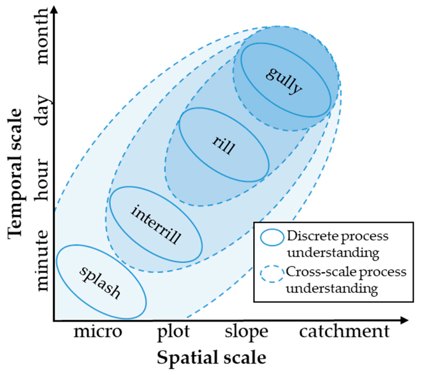
3.2. Soil Erosion Processes

Different soil erosion models are developed for different scales, and therefore vary according to process mapping. Due to the complexity of the occurring and transforming soil erosion processes, the models make simplified assumptions. Splash, interrill, rill and gully erosion vary greatly in their process description [78], with some processes being better presented than others. As displayed in Table 1, there are models such as the DWSM that use coefficients to simulate detachment based on splash and overland flow, while others, such as the EROSION-3D, apply the momentum flux approach. The KINEROS model does not differentiate between interrill and rill erosion [22], whereas WEPP simulates interrill erosion and concentrated runoff within rills but does not take the transition from one to another into account [25]. As presented in Table 1, many models base their process calculation on the kinematic wave, which has been shown as not being sufficient enough for a holistic flow routing. Models developed for small scales depict splash erosion and interrill erosion especially well, whereas those developed for larger scales focus on gully erosion. The following chapter discusses assessment opportunities for an improved process understanding and the feasibility to integrate that information into process-based soil erosion models.

3.2.1. Rill Initiation

Process-based soil erosion models, as displayed in Table 1, show gaps regarding the particle size transport, the deposition, the flow routing and the particle detachment in rills, especially in simulating the initiation of those processes [125]. While most of these models are capable of simulating runoff and soil erosion within existing rills as well as in interrill areas, they lack the ability to depict spontaneous rill formation [21] and the spatial and temporal development of rills. Using a self-organised dynamic system approach [57], RillGrow can map the hydraulic processes inside a rill. However the model is also not capable of simulating rill initiation [21,126]. Wu et al. [127] present an approach on a WEPP-based soil erosion model to simulate erosion and rill evolution on the hillslope scale. For this purpose, they combine an infiltration, a diffusive wave and a modified WEPP model, achieving good agreement regarding erosion, spatial distribution and depth of rills. However, their model has difficulties in locating the initiation, bifurcation and merging of rills [128]. These difficulties stem from the highly random component of rill erosion, which incorporates many different factors [129]. As the spatial and temporal distribution of rills has a significant influence on soil erosion and runoff, the embedding of the initiation and development of rills in soil erosion models is necessary for gaining more precise modelling results [130]. An improved process understanding, gained by repeated and accurate rill erosion assessment [131], and detailed information about their origin, geometry and frequency [25] is an important step in the modelling of rills. Advances in time-lapse SfM allow for the assessment of surface changes during a rainfall event with a temporal resolution of several seconds [108]. Such approaches, as well as information gained by rare earth elements on rill–interrill erosion processes can enable an enhanced temporal and spatial high-resolution process understanding on rill erosion [132]. This knowledge might help to develop and integrate a topographic threshold concept, as was suggested by Nouwakpo et al. [133], to implement the transition from interrill to rill erosion. Lifeng [125] suggests the usage of cellular automata, as in their approach CASEM, to improve the simulation of the initiation of soil erosion processes with a continuously improving system. While promising, this approach is still in the beginning of development. A cross-scale understanding of when and where rills develop, and integrating this knowledge into models, should improve modelling, especially on a spatially distributed level. As previously stated, process-based soil erosion models differ in terms of their process description. Instead of having one improved model, the combination of different adjusted models, similar to the approach of Wu et al. [127], removing the models’ limitations, or Eekhout et al. [134], working with a process-based model ensemble concerning model uncertainties, could prove beneficial. With the available computing capability and the combination of the data, intense but strong sub-models could become an achievable goal.

3.2.2. The Role of Scale Regarding Process Understanding

An improved process understanding can help reduce the necessity of model calibration. Different assessment techniques open up opportunities for an enhanced understanding of soil erosion processes and especially the cross-scale transition from one process to another. Therefore, these new data make it possible to monitor initialising and on-going processes that previously could not be observed at all or “only” in the form of results (e.g., headcut retreat, filling small ponds or aggregates disintegration). Such gained data might be used for model validation and development.
Process-based soil erosion models deliver the best results at the observation scale they were parameterized and validated for [23,78,121,135,136]. Their governing equations are usually derived from the basis of small scales, and transferring them to a different scale can lead to poor validation results [23], because changing the considered scale also changes the prevailing erosional process [25,121]. To understand the dominant processes and their influences on erosional rates, it is important to consider the role of scale. With improving technology, high-resolution data becomes available for a whole range of scales. While these data enable a validated extension of the spatial modelling scales, both on the micro and the macro level [29], it is unclear whether the models are ready for this kind of up and down scaling.
Changing the size of the DEM cell can lead to a different focus on operating processes [29]. An increasing resolution can expose non-erosive processes, e.g., swelling or shrinking, which may mask the actual erosional processes [84]. New assessment techniques should trigger model development for an improved process description. There seems to be an effective resolution which models can cope with and below which small cells show higher erosion rates than is plausible. Models developed for resolutions in the range of metres can have difficulties with very high resolutions. However, a holistic understanding of soil erosion processes, including scale and resolution, remains necessary. Photogrammetric and LiDAR data, as discussed in Section 2, can enable temporal and spatial high resolution change detection and process mapping at different magnitudes [108,137], offering such information for soil erosion modelling. Which scale and resolution to choose from is not only dependent on the research question but also on the models’ capability. While authors already integrated small scale features in large scale modelling, the data base for the viability of such an application in the context of process-based soil erosion modelling remains very limited.
Figure 6 demonstrates how soil erosion processes act within the space-time scale and are superimposed by the next dominant process. While processes occur across scales (dashed lines), soil erosion is usually measured and modelled in a relatively discrete manner (solid lines). So far, insights on the whole scope of soil erosion processes and their interactions between are somewhat limited [138]. Nevertheless, recent assessment developments offer spatial and temporal high-resolution data, which enable the identification and mapping of processes on scales where they have not been visible before. Such techniques provide information not only on the spectrum of erosion and its interaction but also on the spatial and temporal distribution. Different models can be applied to different processes that again work on specific scales. Models consider single slopes or catchments with one mathematical function, as can be seen in Table 1, and reach their limit when switching to the next scale. While different scales are covered by different models and their mathematical equations, a cross-scale modelling approach could be achieved by integrating different parallel existing model equations. Techniques, such as in the area of remote sensing, open up opportunities for cross-scale process understanding and accordingly model integration.

3.3. Connectivity

The complexity and multitude of processes taking place within a catchment affects sediment and water transfer throughout the system. To address management strategies and mitigation measurements, it is necessary to gain a complete overview of the system’s connectivity, shifting the perspective away from the single slope and towards the connected system, taking a variety of spatial scales into account. This leads to a better understanding of the influence of human built structures and natural landforms on the continuity of water and sediment transfer throughout the system as well as the cause of off-site damages [139,140]. Models are simplifications of reality and often neglect the delayed reaction of the sediment yield and the impact of sediment connectivity [136]. Supplementary to erosion rate assessment, the mapping and modelling of sediment transport and runoff throughout the system is very important because those erosional forms have a profound impact on off-site damage [141]. A cross-scale process understanding based on spatial and temporal distributed soil, soil surface and soil erosion assessments can also result in an improved understanding of connectivity and can help to integrate such aspects in process-based soil erosion models.
For a best-fit of sediment transfer to its outlet, Mahoney et al. [142] stress the need of coupling erosion, connectivity formula and flow routing. As Table 1 summarise, the latter shows large gaps across the models and might therefore be tricky to integrate. A modelling approach, which takes connectivity into account, is represented by the GeoWEPP-C model. It combines process-based soil erosion modelling with lateral sediment connectivity modelling but is still in the early stages of development [143]. In order to gain short and long term results from the development of connectivity, Baartman et al. [29] propose a continuous monitoring and modelling of runoff and sediment transfer. GIS-based indices offer an approach to circumvent extensive field work and large amounts of input data to partly quantify relevant connectivity factors [144]. Even though connectivity can currently only be assessed to a certain extent, new high-resolution remote sensing data (e.g., surface change by DEMs) help to measure connectivity aspects at least in parts and enables the development of such connectivity indices [145]. While various methods, including tracing approaches, provide information about connectivity, process-based soil erosion models are not able to integrate this information so easily. This begs the question of whether it is more effective to adapt existing models or to create an entirely new approach, making future models more adaptable to new challenges.

4. Conclusions and Outlook

More advanced techniques as well as opportunities regarding scale and resolution in soil erosion assessment open up new possibilities regarding parameterization and process description. This review provides an overview of the opportunities that the improvement of soil and soil erosion assessment techniques can offer current process-based soil erosion models. We have selected 13 process-based soil erosion models and discussed whether such models can make use of the data presently available. The models have demonstrated different limitations regarding their process understanding, cross-scale modelling and the applicable resolution. We found modelling limitations, e.g., in implementing the calculations (regarding spatial and temporal discretisation), in input data (taking advantage of the available data), regarding the user (the provision of the data is so far very costly) and in the process calculation possibilities, such as the kinematic wave, which is not sufficient enough for a holistic flow routing. They furthermore show difficulties regarding their process choice for the observed scale, which asks for new process integration. An important step could also be the development of a connectivity parameter for the spatial linkage of the modelled erosion. Current data availabilities show potential in addressing some of the aspects models struggle with, such as particle detachment in rills, deposition, connectivity, flow velocity, wind-driven rain, model validation, reducing equifinality and flow routing. We conclude that the amount, availability and assessment of data have been extensively developed over the last few years, especially in the area of photogrammetry, LiDAR and tracing. However, our research has also shown that models can only partly integrate and benefit from new opportunities, such as resolution, and in most cases require a thorough model adaption.
Because the strengths and weaknesses vary between the different models, we see great potential in merging the strengths of the various existing soil erosion models and weaken their limitations by working towards a cross-scale model collection. This could be a combination of different models or take form of an application which integrates the various model equations for different processes on different scales and resolutions. Such a framework, combined with a guideline to the correct choice of equations, based on scale, resolution, available data and the research question, could create a globally applicable adaptive process-based modelling approach. Existing open-source process-based soil erosion models might already be a first step towards such a solution. The complexity of the entire erosional processes cannot be described only on a physical level. This aspect and the large and constantly rising amount of soil erosion data could pave the way towards a new generation of models, which combines data driven frameworks with the strengths of an ensemble of process-based soil erosion models and their physical foundation. In conclusion, future research should focus on advancing model development to keep up with the data and create a more holistic modelling approach.

Author Contributions

Conceptualisation, writing—original draft preparation, visualisation, L.E.; writing—reviewing and editing, L.E., A.K., M.S., A.B., J.L. and A.E.; supervision, A.K., M.S. and A.E. All authors have read and agreed to the published version of the manuscript.

Funding

This research was funded by the Deutsche Forschungsgemeinschaft (DFG, German Research Foundation), grant number KA 5272/1-1 and EL 926/3-1, project number 405774238.

Acknowledgments

We would like to thank the reviewers for the insightful comments that helped us to improve the quality of our paper.

Conflicts of Interest

The authors declare no conflict of interest. The funders had no role in the design of the study; in the collection, analyses, or interpretation of data; in the writing of the manuscript; or in the decision to publish the results.

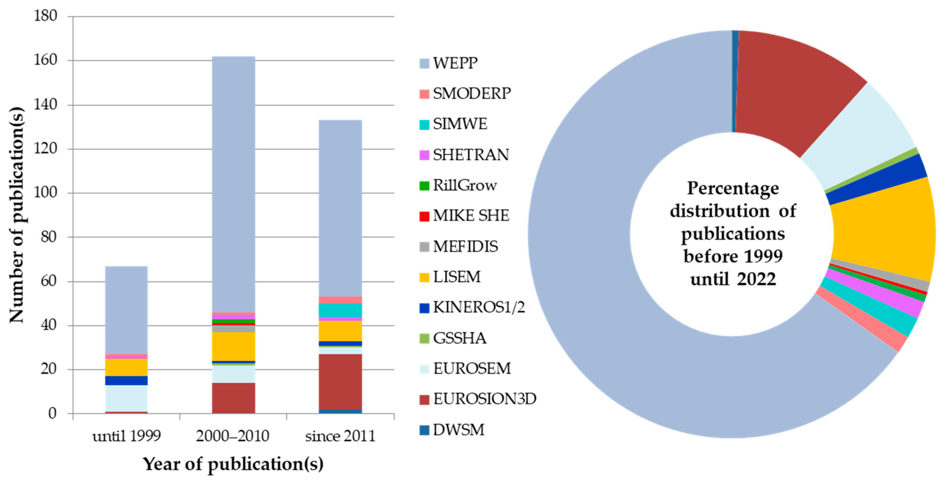
Appendix A. Abbreviations: List of Process-Based Soil Erosion Models

DWSMDynamic Watershed Simulation Model [31]
EROSION-3Dno abbreviation [35]
EUROSEMEuropean Soil Erosion Model [40]
GeoWEPPGeospatial Interface for Water Erosion Prediction Project [144]
GSSHAGridded Surface Subsurface Hydrologic Analysis [44]
KINEROS1/2KINematic runoff and EROsion model [48]
LISEMLimburg Soil Erosion Model [52]
MEFIDISModelo de Erosão FÍsico e DIStribuído [53]
MIKE SHEno abbreviation [56]
RillGrowno abbreviation [57]
SHETRANSysteme Hydrologique Europian-TRANsport [60]
SIMWESIMulation of Water Erosion [61]
SMODERPA Simulation Model of Overland Flow and Erosion Processes [63]
WEPPWater Erosion Prediction Project [66]

References

  1. Swinton, S.M.; Lupi, F.; Robertson, G.P.; Hamilton, S.K. Ecosystem services and agriculture: Cultivating agricultural ecosystems for diverse benefits. Ecol. Econ. 2007, 64, 245–252. [Google Scholar] [CrossRef]
  2. Evans, R.; Brazier, R. Evaluation of modelled spatially distributed predictions of soil erosion by water versus field-based assessments. Environ. Sci. Policy 2005, 8, 493–501. [Google Scholar] [CrossRef] [Green Version]
  3. Evans, D.L.; Quinton, J.N.; Tye, A.M.; Rodés, Á.; Davies, J.A.C.; Mudd, S.M.; Quine, T.A. Arable soil formation and erosion: A hillslope-based cosmogenic nuclide study in the United Kingdom. SOIL 2019, 5, 253–263. [Google Scholar] [CrossRef] [Green Version]
  4. Zhang, X.-C.; Nearing, M.A.; Garbrecht, J.D.; Steiner, J.L. Downscaling Monthly Forecasts to Simulate Impacts of Climate Change on Soil Erosion and Wheat Production. Soil Sci. Soc. Am. J. 2004, 68, 1376–1385. [Google Scholar] [CrossRef] [Green Version]
  5. Guo, M.; Shi, H.; Zhao, J.; Liu, P.; Welbourne, D.; Lin, Q. Digital close range photogrammetry for the study of rill development at flume scale. CATENA 2016, 143, 265–274. [Google Scholar] [CrossRef]
  6. Rieke-Zapp, D.H.; Nearing, M.A. Digital close range photogrammetry for measurement of soil erosion. Photogram. Rec. 2005, 20, 69–87. [Google Scholar] [CrossRef]
  7. Nearing, M.A.; Jetten, V.; Baffaut, C.; Cerdan, O.; Couturier, A.; Hernandez, M.; Le Bissonnais, Y.; Nichols, M.H.; Nunes, J.P.; Renschler, C.S.; et al. Modeling response of soil erosion and runoff to changes in precipitation and cover. CATENA 2005, 61, 131–154. [Google Scholar] [CrossRef]
  8. Routschek, A.; Schmidt, J.; Enke, W.; Deutschlaender, T. Future soil erosion risk—Results of GIS-based model simulations for a catchment in Saxony/Germany. Geomorphology 2014, 206, 299–306. [Google Scholar] [CrossRef]
  9. Li, Z.; Fang, H. Impacts of climate change on water erosion: A review. Earth-Sci. Rev. 2016, 163, 94–117. [Google Scholar] [CrossRef]
  10. Guo, Y.; Peng, C.; Zhu, Q.; Wang, M.; Wang, H.; Peng, S.; He, H. Modelling the impacts of climate and land use changes on soil water erosion: Model applications, limitations and future challenges. J. Environ. Manag. 2019, 250, 109403. [Google Scholar] [CrossRef]
  11. Klik, A.; Eitzinger, J. Impact of climate change on soil erosion and the efficiency of soil conservation practices in Austria. J. Agric. Sci. 2010, 148, 529–541. [Google Scholar] [CrossRef]
  12. Nunes, J.P.; Seixas, J.; Keizer, J.J. Modeling the response of within-storm runoff and erosion dynamics to climate change in two Mediterranean watersheds: A multi-model, multi-scale approach to scenario design and analysis. CATENA 2013, 102, 27–39. [Google Scholar] [CrossRef]
  13. Hu, Y.; Gao, M.; Batunacun. Evaluations of water yield and soil erosion in the Shaanxi-Gansu Loess Plateau under different land use and climate change scenarios. Environ. Dev. 2020, 34, 100488. [Google Scholar] [CrossRef]
  14. Van Oost, K.; Govers, G.; Cerdan, O.; Thauré, D.; van Rompaey, A.; Steegen, A.; Nachtergaele, J.; Takken, I.; Poesen, J. Spatially distributed data for erosion model calibration and validation: The Ganspoel and Kinderveld datasets. CATENA 2005, 61, 105–121. [Google Scholar] [CrossRef]
  15. Mullan, D.; Favis-Mortlock, D.; Fealy, R. Addressing key limitations associated with modelling soil erosion under the impacts of future climate change. Agric. For. Meterol. 2012, 156, 18–30. [Google Scholar] [CrossRef] [Green Version]
  16. Govers, G.; Giménez, R.; van Oost, K. Rill erosion: Exploring the relationship between experiments, modelling and field observations. Earth-Sci. Rev. 2007, 84, 87–102. [Google Scholar] [CrossRef]
  17. Zingg, A.W. Degree and length of land slope as it affects soil loss in run-off. Agric. Enging. 1940, 21, 59–64. [Google Scholar]
  18. Wischmeier, W.H.; Smith, D.D. Predicting Rainfall Erosion Losses from Cropland East of the Rocky Mountains; US Department of Agriculture—Agriculture Research Service: Brooksville, FL, USA, 1965.
  19. Scherer, U. Prozessbasierte Modellierung der Bodenerosion in einer Lösslandschaft. In Dissertation; University Karlsruhe: Karlsruhe, Germany, 2008. [Google Scholar]
  20. De Roo, A.P.J.; Offermans, R.J.E. LISEM: A physically-based hydrological and soil erosion model for basin-scale water and sediment management. Modelling and Management of Sustainable Basin-scale Water Resource Systems. Int. Assoc. Hydrol. Sci. Publ. 1995, 231, 399–407. [Google Scholar]
  21. Pandey, A.; Himanshu, S.K.; Mishra, S.K.; Singh, V.P. Physically based soil erosion and sediment yield models revisited. CATENA 2016, 147, 595–620. [Google Scholar] [CrossRef]
  22. Aksoy, H.; Kavvas, M.L. A review of hillslope and watershed scale erosion and sediment transport models. CATENA 2005, 64, 247–271. [Google Scholar] [CrossRef]
  23. Hajigholizadeh, M.; Melesse, A.M.; Fuentes, H.R. Erosion and Sediment Transport Modelling in Shallow Waters: A Review on Approaches, Models and Applications. Int. J. Environ. Res. Public Health 2018, 15, 518. [Google Scholar] [CrossRef] [PubMed] [Green Version]
  24. Karydas, C.G.; Panagos, P.; Gitas, I.Z. A classification of water erosion models according to their geospatial characteristics. Int. J. Digit. Earth 2012, 7, 229–250. [Google Scholar] [CrossRef]
  25. Merritt, W.S.; Letcher, R.A.; Jakeman, A.J. A review of erosion and sediment transport models. Environ. Modell. Softw. 2003, 18, 761–799. [Google Scholar] [CrossRef]
  26. Borrelli, P.; Alewell, C.; Alvarez, P.; Anache, J.A.A.; Baartman, J.; Ballabio, C.; Bezak, N.; Biddoccu, M.; Cerdà, A.; Chalise, D.; et al. Soil erosion modelling: A global review and statistical analysis. Sci. Total Environ. 2021, 780, 146494. [Google Scholar] [CrossRef]
  27. Parsons, A.J. How reliable are our methods for estimating soil erosion by water? Sci. Total Environ. 2019, 676, 215–221. [Google Scholar] [CrossRef]
  28. Jetten, V.; Favis-Mortlock, D. Modelling Soil Erosion in Europe. In Soil Erosion in Europe; Boardman, J., Poesen, J., Eds.; John Wiley & Sons, Ltd.: Chichester, UK, 2006; pp. 695–716. ISBN 9780470859209. [Google Scholar]
  29. Baartman, J.E.; Nunes, J.P.; Masselink, R.; Darboux, F.; Bielders, C.; Degré, A.; Cantreul, V.; Cerdan, O.; Grangeon, T.; Fiener, P.; et al. What do models tell us about water and sediment connectivity? Geomorphology 2020, 367, 107300. [Google Scholar] [CrossRef]
  30. Batista, P.V.; Laceby, J.P.; Davies, J.; Carvalho, T.S.; Tassinari, D.; Silva, M.L.; Curi, N.; Quinton, J.N. A framework for testing large-scale distributed soil erosion and sediment delivery models: Dealing with uncertainty in models and the observational data. Environ. Modell. Softw. 2021, 137, 104961. [Google Scholar] [CrossRef]
  31. Borah, D.K.; Bera, M.; Shaw, S.; Keefer, L. Dynamic Modeling and Monitoring of Water, Sediment, Nutrients, and Pesticides in Agricultural Watersheds during Storm Events; Illinois Groundwater Consortium: Champaign, IL, USA, 1999. [Google Scholar]
  32. Smith, R.E.; Parlange, J.-Y. A parameter-efficient hydrologic infiltration model. Water Resour. Res. 1978, 14, 533–538. [Google Scholar] [CrossRef]
  33. Lighthill, M.J.; Whitham, G.B. On kinematic waves I. Flood movement in long rivers. Proc. R Soc. Lond. A 1955, 229, 281–316. [Google Scholar] [CrossRef]
  34. Borah, D.K.; Prasad, S.N.; Alonso, C.V. Kinematic wave routing incorporating shock fitting. Water Resour. Res. 1980, 16, 529–541. [Google Scholar] [CrossRef]
  35. Schmidt, J. A mathematical Model to Simulate Rainfall Erosion. Catena Supp. 1991, 19, 101–109. [Google Scholar]
  36. Green, W.H.; Ampt, G.A. Studies on Soil Phyics. J. Agric. Sci. 1911, 4, 1–24. [Google Scholar] [CrossRef] [Green Version]
  37. Schmidt, J. Entwicklung Und Anwendung Eines Physikalisch Begründeten Simulationsmodells Für Die Erosion Geneigter landwirtschaftlicher Nutzflächen; Selbstverl. des Inst. für Geographische Wissenschaften: Berlin, Germany, 1996; ISBN 3-88009-062-9. [Google Scholar]
  38. von Werner, M.; Schröder, A.; Schmidt, J. Abschätzung Des Oberflächenabflusses Und Der Wasserinfiltration Auf Landwirtschaftlich Genutzten Flächen Mit Hilfe Des Modells EROSION-3D Endbericht; Sächsisches Landesamt für Landwirtschaft: Berlin, Germany, 2004; Available online: https://tu-freiberg.de/sites/default/files/media/professur-boden--und-gewaesserschutz-15982/PDF/Publikationen/geognostics_2005.pdf (accessed on 9 April 2020).
  39. Schmidt, J. Modeling long-term soil loss and landform change. In Overland Flow—Hydraulics and Erosion Mechanics; Abrahams, A.J., Parsons, A.D., Eds.; University College London Press: London, UK, 1992. [Google Scholar]
  40. Morgan, R.P.C.; Quinton, J.N.; Smith, R.E.; Govers, G.; Poesen, J.W.; Auerswald, K.; Chisci, G.; Torri, D.; Styczen, M.E.; Folly, A.J. The European Soil Erosion Model (EUROSEM): Documentation and User Guide; Silsoe College, Cranfield University: Bedford, UK, 1998. [Google Scholar]
  41. Woolhiser, D.A.; Liggett, J.A. Unsteady, one-dimensional flow over a plane-The rising hydrograph. Water Resour. Res. 1967, 3, 753–771. [Google Scholar] [CrossRef]
  42. Govers, G. Empirical relationships for the transport capacity of overland flow. Int. Assoc. Hydrol. Sci. Publ. 1990, 189, 45–63. [Google Scholar]
  43. Bagnold, R.A. An Approach to the Sediment Transport Problem from General Physics; Geological Survey Professional paper; US Government Printing Office: Washington, DC, USA, 1966; Volume 1.
  44. Downer, C.W.; Ogden, F.L. GSSHA: Model To Simulate Diverse Stream Flow Producing Processes. J. Hydrol. Eng. 2004, 9, 161–174. [Google Scholar] [CrossRef]
  45. Ogden, F.L.; Saghafian, B. Green and Ampt Infiltration with Redistribution. J. Irrig. Drain. E 1997, 123, 386–393. [Google Scholar] [CrossRef]
  46. Richards, L.A. Capillary conduction of liquids through porous mediums. J. Agric. Sci. 1931, 1, 318–333. [Google Scholar] [CrossRef]
  47. Johnson, B.E.; Julien, P.Y.; Molnar, D.K.; Watson, C.C. The two-dimensional upland erosion model casc2d-sed. J. Am. Water Resour. As. 2000, 36, 31–42. [Google Scholar] [CrossRef]
  48. Woolhiser, D.A.; Smith, R.E.; Goodrich, D.C. KINEROS: A Kinematic Runoff and Erosion Model: Documentation and User Manual; U.S. Department of Agricultural; Agricultural Research Service: Washington, DC, USA, 1990.
  49. Fortuño Ibáñez, J.; Gómez Valentín, M.; Jang, D. Application of the KINEROS 2 Model to Natural Basin for Estimation of Erosion. Appl. Sci. 2021, 11, 9320. [Google Scholar] [CrossRef]
  50. Meyer, L.D.; Wischmeier, W.H. Mathematical Simulation of the Process of Soil Erosion by Water. Trans. ASAE 1969, 732, 754–762. [Google Scholar]
  51. Engelund, F.; Hansen, E. A Monograph on Sediment Transport in Alluvial Streams; Teknisk Vorlag: Copenhagen, Denmark, 1967. [Google Scholar]
  52. De Roo, A.P.J.; Wesseling, C.G.; Cremers, N.H.D.T.; Offermans, R.J.E.; Ritsema, C.J.; Oostindie, K. LISEM: A new physically-based hydrological and soil erosion model in a GIS-environment, theory and implementation. Var. Stream Eros. Sediment Transp. 1994, 224, 439–448. [Google Scholar]
  53. Nunes, J.P.; Vieira, G.N.; Seixas, J.; Gonçalves, P.; Carvalhais, N. Evaluating the MEFIDIS model for runoff and soil erosion prediction during rainfall events. CATENA 2005, 61, 210–228. [Google Scholar] [CrossRef]
  54. Sharma, P.P.; Gupta, S.C.; Rawls, W.J. Soil Detachment by Single Raindrops of Varying Kinetic Energy. Soil Sci. Soc. Am. J. 1991, 55, 301. [Google Scholar] [CrossRef]
  55. Charpa, S.C. Surface Water-Quality Modeling; Waveland Press Inc.: Long Grove, IL, USA, 1997. [Google Scholar]
  56. Abbott, M.B.; Bathurst, J.C.; Cunge, J.A.; O’Connell, P.E.; Rasmussen, J. An introduction to the European Hydrological System—Systeme Hydrologique Europeen, “SHE”, 2: Structure of a physically-based, distributed modelling system. J. Hydrol. 1986, 87, 61–77. [Google Scholar] [CrossRef]
  57. Favis-Mortlock, D. A self-organizing dynamic systems approach to the simulation of rill initiation and development on hillslopes. Comput. Geosci. 1998, 24, 353–372. [Google Scholar] [CrossRef]
  58. Favis-Mortlock, D.T.; Boardman, J.; Parsons, A.J.; Lascelles, B. Emergence and erosion: A model for rill initiation and development. Hydrol. Process. 2000, 14, 2173–2205. [Google Scholar] [CrossRef]
  59. Nearing, M.A.; Norton, L.D.; Bulgakov, D.A.; Larionov, G.A.; West, L.T.; Dontsova, K.M. Hydraulics and erosion in eroding rills. Water Resour. Res. 1997, 33, 865–876. [Google Scholar] [CrossRef]
  60. Bathurst, J.C. Physically-based erosion and sediment yield modelling: The SHETRAN concept. In Modelling Erosion, Sediment Transport and Sediment Yield; Technical Documents in Hydrology: Paris, France, 2002. [Google Scholar]
  61. Mitas, L.; Mitasova, H. Distributed soil erosion simulation for effective erosion prevention. Water Resour. Res. 1998, 34, 505–516. [Google Scholar] [CrossRef]
  62. Julien, P.Y.; Saghafian, B.; Ogden, F.L. Raster-based hydrologic modeling of spatially-varied surface runoff. J. Am. Water Resour. Assoc. 1995, 31, 523–536. [Google Scholar] [CrossRef]
  63. Dostál, T.; Váška, J.; Vrána, K. SMODERP—A Simulation Model of Overland Flow and Erosion Processes. In Soil Erosion; Schmidt, J., Ed.; Springer: Berlin/Heidelberg, Germany, 2000; pp. 135–161. ISBN 978-3-642-08605-2. [Google Scholar]
  64. Kavka, P.; Zajicek, J. Soil erosion model smoderp—1D and 2D modelling. In Proceedings of the 13th International Multidisciplinary Scientific GeoConference SGEM, Albena, Bulgaria, 16–22 June 2013. [Google Scholar] [CrossRef]
  65. Philip, J.R. The theory of infiltration. Soil Sci. 1957, 83, 345–358. [Google Scholar] [CrossRef]
  66. Laflen, J.M.; Lane, L.J.; Foster, G.R. WEPP: A new generation of erosion prediction technology. J. Soil Water Conserv. 1991, 46, 34–38. [Google Scholar]
  67. Flanagan, D.C.; Ascough, J.C.; Nearing, M.A.; Laflen, J.M. The Water Erosion Prediction Project (WEPP) Model. In Landscape Erosion and Evolution Modeling; Harmon, R.S., Doe, W.W., Eds.; Springer: Boston, MA, USA, 2001; pp. 145–199. ISBN 978-1-4613-5139-9. [Google Scholar]
  68. Chu, S.T. Infiltration during an unsteady rain. Water Resour. Res. 1978, 14, 461–466. [Google Scholar] [CrossRef]
  69. Foster, G.R.; Flanagan, D.C.; Nearing, M.; Lane, L.J.; Risse, L.M.; Finker, S.C. Hillslope erosion component. In USDA-Water Erosion Prediction Project: Hillslope Profile and Watershed Model Documentation; USDA-ARS National Soil Erosion Research Laboratory: West Lafayette, IN, USA, 1995. [Google Scholar]
  70. Yalin, M.S. An Expression for Bed-Load Transportation. J. Hydraul. Div. 1963, 89, 221–250. [Google Scholar] [CrossRef]
  71. Li, Y.; Bai, X.; Tian, Y.; Luo, G. Review and Future Research Directions about Major Monitoring Method of Soil Erosion. J. Hydrol. Eng. 2017, 63, 12042. [Google Scholar] [CrossRef] [Green Version]
  72. Padarian, J.; Minasny, B.; McBratney, A.B. Machine learning and soil sciences: A review aided by machine learning tools. SOIL 2020, 6, 35–52. [Google Scholar] [CrossRef] [Green Version]
  73. Castillo, C.; Pérez, R.; James, M.R.; Quinton, J.N.; Taguas, E.V.; Gómez, J.A. Comparing the Accuracy of Several Field Methods for Measuring Gully Erosion. Soil Sci. Soc. Am. J. 2012, 76, 1319–1332. [Google Scholar] [CrossRef] [Green Version]
  74. Rodrigo-Comino, J. Five decades of soil erosion research in “terroir”. The State-of-the-Art. Earth-Sci. Rev. 2018, 179, 436–447. [Google Scholar] [CrossRef]
  75. Guan, Z.; Tang, X.-Y.; Yang, J.E.; Ok, Y.S.; Xu, Z.; Nishimura, T.; Reid, B.J. A review of source tracking techniques for fine sediment within a catchment. Environ. Geochem. Health 2017, 39, 1221–1243. [Google Scholar] [CrossRef] [Green Version]
  76. Jester, W.; Klik, A. Soil surface roughness measurement—Methods, applicability, and surface representation. CATENA 2005, 64, 174–192. [Google Scholar] [CrossRef]
  77. Thomsen, L.M.; Baartman, J.E.M.; Barneveld, R.J.; Starkloff, T.; Stolte, J. Soil surface roughness: Comparing old and new measuring methods and application in a soil erosion model. SOIL 2015, 1, 399–410. [Google Scholar] [CrossRef] [Green Version]
  78. Batista, P.V.; Davies, J.; Silva, M.L.; Quinton, J.N. On the evaluation of soil erosion models: Are we doing enough? Earth-Sci. Rev. 2019, 197, 102898. [Google Scholar] [CrossRef]
  79. Loughran, R.J. The measurement of soil erosion. Prog. Phys. Geogr. Earth Environ. 1989, 13, 216–233. [Google Scholar] [CrossRef]
  80. Septianugraha, R.; Harryanto, R.; Sara, D.S. Remote sensing and GIS methode for assess erosion with satellite imagery at Citarik Sub-Watershed. IOP Conference Series: Earth and Environmental Science, Bandung, Indonesia, 5–7 August 2019; Volume 393, p. 12064. [Google Scholar] [CrossRef]
  81. Zhou, T.; Geng, Y.; Chen, J.; Pan, J.; Haase, D.; Lausch, A. High-resolution digital mapping of soil organic carbon and soil total nitrogen using DEM derivatives, Sentinel-1 and Sentinel-2 data based on machine learning algorithms. Sci. Total Environ. 2020, 729, 138244. [Google Scholar] [CrossRef]
  82. Gholizadeh, A.; Žižala, D.; Saberioon, M.; Borůvka, L. Soil organic carbon and texture retrieving and mapping using proximal, airborne and Sentinel-2 spectral imaging. Remote Sens. Environ. 2018, 218, 89–103. [Google Scholar] [CrossRef]
  83. Hu, Y.; Fister, W.; He, Y.; Kuhn, N.J. Assessment of crusting effects on interrill erosion by laser scanning. Peer J. 2020, 8, e8487. [Google Scholar] [CrossRef]
  84. Kaiser, A.; Erhardt, A.; Eltner, A. Addressing uncertainties in interpreting soil surface changes by multitemporal high-resolution topography data across scales. Land Degrad. Dev. 2018, 29, 2264–2277. [Google Scholar] [CrossRef]
  85. Li, L.; Nearing, M.A.; Nichols, M.H.; Polyakov, V.O.; Phillip Guertin, D.; Cavanaugh, M.L. The effects of DEM interpolation on quantifying soil surface roughness using terrestrial LiDAR. Soil Till. Res. 2020, 198, 104520. [Google Scholar] [CrossRef]
  86. Gilliot, J.M.; Vaudour, E.; Michelin, J. Soil surface roughness measurement: A new fully automatic photogrammetric approach applied to agricultural bare fields. Comput. Electron. Agric. 2017, 134, 63–78. [Google Scholar] [CrossRef]
  87. Eltner, A.; Schneider, D.; Maas, H.-G. Integrated Processing of High Resolution Topographic Data for Soil Erosion Assessment Considering Data Acquisition Schemes and Surface Properties. Int. Arch. Photogramm. Remote Sens. Spatial. Inf. Sci. 2016, XLI-B5, 813–819. [Google Scholar] [CrossRef] [Green Version]
  88. Onnen, N.; Eltner, A.; Heckrath, G.; van Oost, K. Monitoring soil surface roughness under growing winter wheat with low-altitude UAV sensing: Potential and limitations. Earth Surf. Proc. Land 2020, 45, 3747–3759. [Google Scholar] [CrossRef]
  89. Kemppinen, J.; Niittynen, P.; Riihimäki, H.; Luoto, M. Modelling soil moisture in a high-latitude landscape using LiDAR and soil data. Earth Surf. Proc. Land 2018, 43, 1019–1031. [Google Scholar] [CrossRef]
  90. Ge, Y.; Thomasson, J.A.; Sui, R. Remote sensing of soil properties in precision agriculture: A review. Front. Earth Sci. 2011, 33, 149. [Google Scholar] [CrossRef]
  91. Meinen, B.U.; Robinson, D.T. Mapping erosion and deposition in an agricultural landscape: Optimization of UAV image acquisition schemes for SfM-MVS. Remote Sens. Environ. 2020, 239, 111666. [Google Scholar] [CrossRef]
  92. Alexakis, D.D.; Tapoglou, E.; Vozinaki, A.-E.K.; Tsanis, I.K. Integrated Use of Satellite Remote Sensing, Artificial Neural Networks, Field Spectroscopy, and GIS in Estimating Crucial Soil Parameters in Terms of Soil Erosion. Remote Sens. 2019, 11, 1106. [Google Scholar] [CrossRef] [Green Version]
  93. Bondi, G.; Creamer, R.; Ferrari, A.; Fenton, O.; Wall, D. Using machine learning to predict soil bulk density on the basis of visual parameters: Tools for in-field and post-field evaluation. Geoderma 2018, 318, 137–147. [Google Scholar] [CrossRef]
  94. de Lima, R.L.P.; Abrantes, J.R.; de Lima, J.L.M.P.; de Lima, M.I.P. Using thermal tracers to estimate flow velocities of shallow flows: Laboratory and field experiments. J. Hydrol. Hydromech. 2015, 63, 255–262. [Google Scholar] [CrossRef] [Green Version]
  95. Tauro, F.; Grimaldi, S. Ice dices for monitoring stream surface velocity. J. Hydro-Environ. Res. 2016, 14, 143–149. [Google Scholar] [CrossRef]
  96. Lin, D.; Eltner, A.; Sardemann, H.; Maas, H.-G. Automatic spatio-temporal flow velocity measurement in small rivers using thermal image sequences. ISPRS Ann. Photogramm. Remote Sens. Spatial. Inf. Sci. 2018, IV-2, 201–208. [Google Scholar] [CrossRef] [Green Version]
  97. Mabit, L.; Benmansour, M.; Walling, D.E. Comparative advantages and limitations of the fallout radionuclides (137)Cs, (210)Pb(ex) and (7)Be for assessing soil erosion and sedimentation. J. Environ. Radioactiv. 2008, 99, 1799–1807. [Google Scholar] [CrossRef]
  98. Alewell, C.; Pitois, A.; Meusburger, K.; Ketterer, M.; Mabit, L. 239+240 Pu from “contaminant” to soil erosion tracer: Where do we stand? Earth Sci. Rev. 2017, 172, 107–123. [Google Scholar] [CrossRef]
  99. Deumlich, D.; Jha, A.; Kirchner, G. Comparing measurements, 7Be radiotracer technique and process-based erosion model for estimating short-term soil loss from cultivated land in Northern Germany. Soil Water Res. 2017, 12, 177–186. [Google Scholar] [CrossRef] [Green Version]
  100. Baumgart, P.; Eltner, A.; Domula, A.R.; Barkleit, A.; Faust, D. Scale dependent soil erosion dynamics in a fragile loess landscape. Z. Für Geomorphol. 2017, 61, 191–206. [Google Scholar] [CrossRef]
  101. Guzmán, G.; Quinton, J.N.; Nearing, M.A.; Mabit, L.; Gómez, J.A. Sediment tracers in water erosion studies: Current approaches and challenges. J. Soil Sediment 2013, 13, 816–833. [Google Scholar] [CrossRef]
  102. Sepuru, T.K.; Dube, T. An appraisal on the progress of remote sensing applications in soil erosion mapping and monitoring. Remote Sens. Appl. Soc. Environ. 2018, 9, 1–9. [Google Scholar] [CrossRef]
  103. Vrieling, A. Satellite remote sensing for water erosion assessment: A review. CATENA 2006, 65, 2–18. [Google Scholar] [CrossRef]
  104. Eekhout, J.P.C.; Terink, W.; de Vente, J. Assessing the large-scale impacts of environmental change using a coupled hydrology and soil erosion model. Earth Surf. Dynam. 2018, 6, 687–703. [Google Scholar] [CrossRef] [Green Version]
  105. Neugirg, F.; Kaiser, A.; Schmidt, J.; Becht, M.; Haas, F. Quantification, analysis and modelling of soil erosion on steep slopes using LiDAR and UAV photographs. Proc. IAHS 2015, 367, 51–58. [Google Scholar] [CrossRef] [Green Version]
  106. Glendell, M.; McShane, G.; Farrow, L.; James, M.R.; Quinton, J.; Anderson, K.; Evans, M.; Benaud, P.; Rawlins, B.; Morgan, D.; et al. Testing the utility of structure-from-motion photogrammetry reconstructions using small unmanned aerial vehicles and ground photography to estimate the extent of upland soil erosion. Earth Surf. Processes Landf. 2017, 42, 18601871. [Google Scholar] [CrossRef]
  107. Eltner, A.; Sofia, G. Structure from motion photogrammetric technique. In Remote Sensing of Geomorphology; Elsevier: Amsterdam, The Netherlands, 2020; pp. 1–24. ISBN 9780444641779. [Google Scholar]
  108. Eltner, A.; Kaiser, A.; Abellan, A.; Schindewolf, M. Time lapse structure-from-motion photogrammetry for continuous geomorphic monitoring. Earth Surf. Proc. Land 2017, 42, 2240–2253. [Google Scholar] [CrossRef]
  109. Yang, Y.; Shi, Y.; Liang, X.; Huang, T.; Fu, S.; Liu, B. Evaluation of structure from motion (SfM) photogrammetry on the measurement of rill and interrill erosion in a typical loess. Geomorphology 2021, 385, 107734. [Google Scholar] [CrossRef]
  110. Laburda, T.; Krása, J.; Zumr, D.; Devátý, J.; Vrána, M.; Zambon, N.; Johannsen, L.L.; Klik, A.; Strauss, P.; Dostál, T. SfM-MVS Photogrammetry for Splash Erosion Monitoring under Natural Rainfall. Earth Surf. Proc. Land 2021, 46, 1067–1082. [Google Scholar] [CrossRef]
  111. Li, L.; Nearing, M.A.; Nichols, M.H.; Polyakov, V.O.; Cavanaugh, M.L. Using terrestrial LiDAR to measure water erosion on stony plots under simulated rainfall. Earth Surf. Proc. Land 2020, 45, 484–495. [Google Scholar] [CrossRef]
  112. Vinci, A.; Brigante, R.; Todisco, F.; Mannocchi, F.; Radicioni, F. Measuring rill erosion by laser scanning. CATENA 2015, 124, 97–108. [Google Scholar] [CrossRef]
  113. Kaiser, A.; Neugirg, F.; Haas, F.; Schmidt, J.; Becht, M.; Schindewolf, M. Determination of hydrological roughness by means of close range remote sensing. SOIL 2015, 1, 613–620. [Google Scholar] [CrossRef] [Green Version]
  114. Blanch, X.; Eltner, A.; Guinau, M.; Abellan, A. Multi-Epoch and Multi-Imagery (MEMI) Photogrammetric Workflow for Enhanced Change Detection Using Time-Lapse Cameras. Remote Sens. 2021, 13, 1460. [Google Scholar] [CrossRef]
  115. Marzen, M.; Iserloh, T.; de Lima, J.L.M.P.; Fister, W.; Ries, J.B. Impact of severe rain storms on soil erosion: Experimental evaluation of wind-driven rain and its implications for natural hazard management. Sci. Total Environ. 2017, 590–591, 502–513. [Google Scholar] [CrossRef]
  116. Schmidt, J.; Werner, M.v.; Schindewolf, M. Wind effects on soil erosion by water—A sensitivity analysis using model simulations on catchment scale. CATENA 2017, 148, 168–175. [Google Scholar] [CrossRef]
  117. Alewell, C.; Borrelli, P.; Meusburger, K.; Panagos, P. Using the USLE: Chances, challenges and limitations of soil erosion modelling. Int. Soil Water Cons. Res. 2019, 7, 203–225. [Google Scholar] [CrossRef]
  118. Starkloff, T.; Stolte, J. Applied comparison of the erosion risk models EROSION 3D and LISEM for a small catchment in Norway. CATENA 2014, 118, 154–167. [Google Scholar] [CrossRef] [Green Version]
  119. Ayensa-Jiménez, J.; Doweidar, M.H.; Sanz-Herrera, J.A.; Doblaré, M. An unsupervised data completion method for physically-based data-driven models. Comput. Method Appl. M 2019, 344, 120–143. [Google Scholar] [CrossRef] [Green Version]
  120. Hessel, R.; van den Bosch, R.; Vigiak, O. Evaluation of the LISEM soil erosion model in two catchments in the East African Highlands. Earth Surf. Proc. Land 2006, 31, 469–486. [Google Scholar] [CrossRef]
  121. Govers, G. Misapplications and Misconceptions of Erosion Models. In Handbook of Erosion Modelling; Morgan, R.P.C., Nearing, M.A., Eds.; John Wiley & Sons, Ltd.: Chichester, UK, 2010; pp. 117–134. ISBN 9781444328455. [Google Scholar]
  122. Starkloff, T.; Stolte, J.; Hessel, R.; Ritsema, C.; Jetten, V. Integrated, spatial distributed modelling of surface runoff and soil erosion during winter and spring. CATENA 2018, 166, 147–157. [Google Scholar] [CrossRef]
  123. Favis-Mortlock, D. “The Right Answer for the Wrong Reason” Revisited: Validation of a Spatially-Explicit Soil Erosion Model (RillGrow); EGU: Vienna, Austria, 2010. [Google Scholar]
  124. Culling, W.E.H. Multicyclic Streams and the Equilibrium Theory of Grade. J. Geol. 1957, 65, 259–274. [Google Scholar] [CrossRef]
  125. Lifeng, Y. A soil erosion model based on cellular automata. Int. Arch. Photogramm. Remote Sens. Spat. Inf. Sci. 2008, 37, 21–26. [Google Scholar]
  126. Wirtz, S.; Seeger, M.; Ries, J.B. The rill experiment as a method to approach a quantification of rill erosion process activity. Z. Für Geomorphol. 2010, 54, 47–64. [Google Scholar] [CrossRef]
  127. Wu, S.; Chen, L.; Wang, N.; Yu, M.; Assouline, S. Modeling Rainfall-Runoff and Soil Erosion Processes on Hillslopes With Complex Rill Network Planform. Water Resour. Res. 2018, 54, 570. [Google Scholar] [CrossRef]
  128. Wu, S.; Chen, L.; Wang, N.; Li, J.; Li, J. Two-dimensional rainfall-runoff and soil erosion model on an irregularly rilled hillslope. J. Hydrol. 2020, 580, 124346. [Google Scholar] [CrossRef]
  129. Wirtz, S.; Seeger, M.; Zell, A.; Wagner, C.; Wagner, J.-F.; Ries, J.B. Applicability of different hydraulic parameters to describe soil detachment in eroding rills. PLoS ONE 2013, 8, e64861. [Google Scholar] [CrossRef] [Green Version]
  130. Wu, S.; Chen, L. Modeling Soil Erosion With Evolving Rills on Hillslopes. Water Resour. Res. 2020, 56, 697. [Google Scholar] [CrossRef]
  131. Di Stefano, C.; Ferro, V.; Palmeri, V.; Pampalone, V. Measuring rill erosion using structure from motion: A plot experiment. CATENA 2017, 156, 383–392. [Google Scholar] [CrossRef]
  132. Zhang, X.-C.J.; Liu, G.; Zheng, F. Understanding erosion processes using rare earth element tracers in a preformed interrill-rill system. Sci. Total Environ. 2018, 625, 920–927. [Google Scholar] [CrossRef] [PubMed]
  133. Nouwakpo, S.K.; Williams, C.J.; Al-Hamdan, O.Z.; Weltz, M.A.; Pierson, F.; Nearing, M. A review of concentrated flow erosion processes on rangelands: Fundamental understanding and knowledge gaps. Int. Soil Water Cons. Res. 2016, 4, 75–86. [Google Scholar] [CrossRef] [Green Version]
  134. Eekhout, J.P.; Millares-Valenzuela, A.; Martínez-Salvador, A.; García-Lorenzo, R.; Pérez-Cutillas, P.; Conesa-García, C.; Vente, J. A process-based soil erosion model ensemble to assess model uncertainty in climate-change impact assessments. Land Degrad. Dev. 2021, 32, 2409–2422. [Google Scholar] [CrossRef]
  135. Cerdà, A.; Brazier, R.; Nearing, M.; de Vente, J. Scales and erosion. CATENA 2013, 102, 1–2. [Google Scholar] [CrossRef]
  136. de Vente, J.; Poesen, J.; Verstraeten, G.; Govers, G.; Vanmaercke, M.; van Rompaey, A.; Arabkhedri, M.; Boix-Fayos, C. Predicting soil erosion and sediment yield at regional scales: Where do we stand? Earth-Sci. Rev. 2013, 127, 16–29. [Google Scholar] [CrossRef]
  137. Kou, P.; Xu, Q.; Yunus, A.P.; Ju, Y.; Guo, C.; Wang, C.; Zhao, K. Multi-temporal UAV data for assessing rapid rill erosion in typical gully heads on the largest tableland of the Loess Plateau, China. Bull. Eng. Geol. Environ. 2020, 79, 1861–1877. [Google Scholar] [CrossRef]
  138. Fernández-Raga, M.; Palencia, C.; Keesstra, S.; Jordán, A.; Fraile, R.; Angulo-Martínez, M.; Cerdà, A. Splash erosion: A review with unanswered questions. Earth-Sci. Rev. 2017, 171, 463–477. [Google Scholar] [CrossRef] [Green Version]
  139. Cavalli, M.; Vericat, D.; Pereira, P. Mapping water and sediment connectivity. Sci. Total Environ. 2019, 673, 763–767. [Google Scholar] [CrossRef]
  140. Biddulph, M.; Collins, A.L.; Foster, I.; Holmes, N. The scale problem in tackling diffuse water pollution from agriculture: Insights from the Avon Demonstration Test Catchment programme in England. River Res. Appl. 2017, 33, 1527–1538. [Google Scholar] [CrossRef] [Green Version]
  141. Boardman, J.; Vandaele, K.; Evans, R.; Foster, I.D.L. Off-site impacts of soil erosion and runoff: Why connectivity is more important than erosion rates. Soil Use Manag. 2019, 35, 245–256. [Google Scholar] [CrossRef] [Green Version]
  142. Mahoney, D.T.; Fox, J.; Al-Aamery, N.; Clare, E. Integrating connectivity theory within watershed modelling part II: Application and evaluating structural and functional connectivity. Sci. Total Environ. 2020, 740, 140386. [Google Scholar] [CrossRef]
  143. Poeppl, R.E.; Dilly, L.A.; Haselberger, S.; Renschler, C.S.; Baartman, J.E.M. Combining Soil Erosion Modeling with Connectivity Analyses to Assess Lateral Fine Sediment Input into Agricultural Streams. Water 2019, 11, 1793. [Google Scholar] [CrossRef] [Green Version]
  144. Najafi, S.; Dragovich, D.; Heckmann, T.; Sadeghi, S.H. Sediment connectivity concepts and approaches. CATENA 2021, 196, 104880. [Google Scholar] [CrossRef]
  145. Heckmann, T.; Cavalli, M.; Cerdan, O.; Foerster, S.; Javaux, M.; Lode, E.; Smetanová, A.; Vericat, D.; Brardinoni, F. Indices of sediment connectivity: Opportunities, challenges and limitations. Earth-Sci. Rev. 2018, 187, 77–108. [Google Scholar] [CrossRef] [Green Version]
Figure 1. Number of process-based soil erosion models developed over the decades between 1970 and 2018 based on Aksoy and Kavvas [22] (p. 253), Hajigholizadeh et al. [23] (pp. 11–13), Karydas et al. [24] (p. 10), Merritt et al. [25] (pp. 766, 791) and Pandey et al. [21] (pp. 600–606). The number of models developed before 1970 is very small and has therefore been ignored.
Remotesensing 14 02468 g001
Figure 2. Literature analysis based on the Google Scholar search engine. Search query (28 April 2022) including model abbreviation and “erosion” limited to “all in title” findings for the years up to 1999, between 2000 and 2010 and since the year 2011 until now. The analysis includes the number of publications found in each time frame on the left-hand side, and the percentage of each models’ application all together on the right. The colouring on the left is arranged from the bottom to the top (DWSM to WEPP), on the right it starts at the top reading clockwise (DWSM to WEPP).
Remotesensing 14 02468 g002
Figure 3. Overview of soil and soil erosion assessment techniques, structured by their type of assessment, their output (area average, selective or distributed) and their temporal scale. The methods presented in this figure are not weighted and do not claim to be exhaustive. The selection is based on Guan et al. [75], Li et al. [71], Jester and Klik [76], Thomsen et al. [77], Batista et al. [78] and Rodrigo-Comino [74].
Remotesensing 14 02468 g003
Figure 4. Changes and developments in soil erosion assessment techniques as well as their temporal and spatial scales of application, (left) derived from Loughran [79] presenting assessment techniques used in 1989 and (right) based on information from Guan et al. [75], Li et al. [71], Jester and Klik [76], Thomsen et al. [77], Batista et al. [78], Rodrigo-Comino [74] and, as discussed in Section 2.2.1 and Section 2.2.2, methods used up to 2017. The methods are coloured by their type of output (area average, selective or distributed). The category discharge measurement includes aspects such as erosion plots and techniques, also listed in Figure 3 under the heading of sediment collecting.
Remotesensing 14 02468 g004
Figure 5. Literature analysis based on the Google Scholar search engine. Search query (28 April 2022) including the name of the assessment techniques (full name, abbreviations) and “erosion” limited to “all in title” findings for the years up to 1999, between 2000 and 2010 and since the year 2011 until now. The analysis includes the number of publications found in each time frame on the left-hand side, and the percentage of the mentioning of each model all together on the right-hand side. LiDAR includes terrestrial and airborne laser scanning. The different categories researched can be found in more detail in Figure 3. The colouring on the left is arranged from the bottom to the top (LiDAR to Others); on the right it starts at the top reading clockwise (LiDAR to Others).
Remotesensing 14 02468 g005
Figure 6. Soil erosion processes considered by taking their cross-scale interaction into account (dashed ellipses) as well as the discrete consideration within their dominant temporal and spatial scale (continuous ellipses). Assessment techniques such as splash cups, discharge measurement, roller chain and topographical survey, as well as process-based soil erosion models, have a discrete process understanding, whereas methods as remote sensing of tracing offer a cross-scale process understanding.
Remotesensing 14 02468 g006
Table 1. Process-based (distributed and event-based) soil erosion models and their basic equations regarding their processes mapping (coefficient = coef., equation = eq.). The meaning of the models’ acronyms can be found in Appendix A. The table is derived from the process-based soil erosion models reviewed by Aksoy and Kavvas [22], Karydas et al. [24], Hajigholizadeh et al. [23], Merritt et al. [25] and Pandey et al. [21]. To ensure a good overview, only models with at least 10 publications since 2000 were included in the following table.
Model InformationField/ Watershed ScaleProcess Mapping
Infiltration (Matrix Infiltration (MI))Runoff Generation and Delay (Flow Velocity (FV), Runoff Delay (RD))Particle Detachment by Splash and by Overland Flow (DbS & DbO)Particle Size & Sediment Transport (PT & ST), Particle Size Distribution [PD]Sediment Deposition (SD) & Particle Size Distribution (PD)Flow Routing (FR) (Channel Routing
(CR), Overland Flow Routing (OfR))
DWSM
[31]
WMI: Smith-Parlange [32]FV: Manning’s n [31]; RD: kinematic wave [33]DbS: raindrop detachment coef.; DbO: flow detachment coef. [31]ST: sediment continuity eq.; PT: bed load formula [31]SD & PD: volumetric rate of sediment deposition per unit length [29]FR: water routing scheme (approximate shock-fitting) [34], modified PULS routing [31]
EROSION -3D [35]F/WMI: Green Ampt [36]FV: Manning’s n [37]; RD: kinematic wave [38]DbS & DbO: momentum flux approach [39]ST: transport capacity; PT: Stokes eq. [37]SD: transport capacity; PD: deposition coef. [37]DEM (digital elevation model) based OfR: FD8; CF: D8 [37]
EUROSEM [40]FMI: Smith-Parlange [32]FV: Manning’s n [40]; RD: kinematic wave [41]DbS: raindrop impact eq. [40]; DbO: generalised erosion theory [40]ST: modified stream power [42,43]; PD: finite difference eq. [40]SD: generalised deposition theory [40]FR: rating equation based on normal flow eq. [40]
GSSHA
[44]
WMI: (traditional/ modified) Green Ampt [36,45]; 1-D Richards eq. [46]FV: Manning’s n [44] No information foundST: modified Klinic -Richardson (incl. empirical coef.) [44]; PD: unit stream power method [44]SD: trap efficiency
relation [47]
OfR: 2D diffusive wave [44]; CR: 1-D up-gradient explicit diffusive wave [44]
KINEROS 1/2
[48,49]
WMI: Smith-Parlange [32]FV: Manning’s n, Reynolds number, Chezy C [48]; RD: kinematic wave [41] DbS: empirical function [48]; DbO: mass-balance eq. kinetic transfer process [48] ST: tractive force relation [50], unit stream power relation, Bagnold relation, Ackers & White relation, transport relation [48], Engelund -Hansen transport relation [51] SD: transport capacity; PD: deposition coef. [48]CR: kinematic approximation to the eq. of unsteady [48]
LISEM
[20,52]
WMI: Richards eq. (part Mualem/ Van Genuchten eq.) [52]FV, Manning’s n; RD: kinematic wave (four-point finite-difference solution) [52]DbS: splash detachment function [20]; DbO: generalised erosion theory [40]ST: transport capacity (unit stream power function); PD: function of grain size [42]SD: generalised deposition theory [40]; PD: transport capacity [42]No information found
MEFIDIS
[53]
WMI: Green Ampt [53]FV: Manning’s n; RD: kinematic wave [53]DbS: raindrop eq.; DbO: interrill sediment delivery eq. [54]ST: transport capacity eq. [42]; PD: particle sedimentation velocity (Stoke’s law) [55]SD: transport capacity eq. [42]; PD: particle sedimentation velocity (Stoke’s law) [55]Runoff generation and routing: Saint Venant eq. [53]
MIKE SHE
[56]
F/WMI: 1-D Richards eq.; macropore infiltration: simplified capacitance-type approach [56]FV: Manning’s n; RD: Saint Venant eq. (1-D and 2-D), diffusive wave approximation, kinematic wave [56]DbS & DbO: Saint Venant eq. of continuity and momentum, implicit finite difference scheme [56]ST: 3-D Darcy eq. [56]; channel flow: 1-D hydrological model MIKE 11 [56]No information foundNo information found
RillGrow
[57]
FInfiltration is ignored [57]FV: base component and depth-dependent component [58]DbO: S-curve stream-power-based expression [59]ST & PD: unit sediment load, infinite transport capacity [59]No implementation [57]FR: routing algorithm [58], self-organising dynamic system [57]
SHETRAN
[60]
F/WMI: 1-D Richard’s eq. [60]RD: Saint Venant eq. (1-D and 2-D) [60]DbS: raindrop impact soil erodibility coef., [60]; DbO: overland flow soil erodibility coef. [60]ST & PD: mass conservation eq., incorporating Engelund-Hansen total load & Yalin bed load transport capacity eq. [60]SD & PD: mass conservation eq., incorporating Engelund-Hansen total load & Yalin bed load transport capacity eq. [60]No information found
SIMWE [61]WNo information foundFV: based on Manning’s n; RD: kinematic wave (+diffusion coef.) [61]DbS & DbO: detachment capacity coef. [61] ST: transport capacity; PD: continuity of sediment mass eq. [61]SD: transport capacity [61]FR: flow as bivariate vector fields [62]
SMODERP 1/2 [63,64]F/WMI: Philip eq. [65]FV: Manning’s n; RD: kinematic wave, Saint Venant eq. (motion and continuity eq.) [64]DbS & DbO: amount of detached soil particles eq. [63]ST: transport capacity; PD: movement of soil particles [63]SD: transport capacity; PD: sedimentation of soil particles [63]DEM based OfR: D8 flow direction algorithm [63]
WEPP
[66,67]
F/WMI: modified Green Ampt Mein-Larson model [68]FV: random roughness; RD: (semi-analytic/ approximation) kinematic wave [66]DbS: Darcy -Weisbach friction factors and shear stress [69]; DbO: linear function of excess hydraulic shear [66]ST: Yalin sediment transport eq. [70]; PD: fall velocity of transported sediment [66]SD: transport capacity; PD: sediment particle sorting due to selective deposition [67]No information found
Publisher’s Note: MDPI stays neutral with regard to jurisdictional claims in published maps and institutional affiliations.

