Extraction of Broad-Leaved Tree Crown Based on UAV Visible Images and OBIA-RF Model: A Case Study for Chinese Olive Trees

Abstract

Chinese olive trees (Canarium album L.) are broad-leaved species that are widely planted in China. Accurately obtaining tree crown information provides important data for evaluating Chinese olive tree growth status, water and fertilizer management, and yield estimation. To this end, this study first used unmanned aerial vehicle (UAV) images in the visible band as the source of remote sensing (RS) data. Second, based on spectral features of the image object, the vegetation index, shape, texture, and terrain features were introduced. Finally, the extraction effect of different feature dimensions was analyzed based on the random forest (RF) algorithm, and the performance of different classifiers was compared based on the features after dimensionality reduction. The results showed that the difference in feature dimensionality and importance was the main factor that led to a change in extraction accuracy. RF has the best extraction effect among the current mainstream machine learning (ML) algorithms. In comparison with the pixel-based (PB) classification method, the object-based image analysis (OBIA) method can extract features of each element of RS images, which has certain advantages. Therefore, the combination of OBIA and RF algorithms is a good solution for Chinese olive tree crown (COTC) extraction based on UAV visible band images.

1. Introduction

Broad-leaved species are a common type in forestry resources. One of the most economic tree species in China are broad-leaved trees with flat, broad leaves, compared to conifers with long and slender leaves [1,2,3]. Among them, Chinese olive (Canarium album L.)—a typical broad-leaved species—have high economic and medicinal value [4,5]. The crown is an essential part of the tree, and is important for physiological processes such as photosynthesis, respiration, and transpiration. It reflects the growth status of individual trees, the degree of their adaptation, and variation to different growth environments, and it is a critical parameter for predicting the growth status and increment of trees [6,7]. Here, by obtaining individual tree crown parameters, we constructed a corresponding standing tree volume model using the crown area and other parameters. It is of great significance to estimate forest stand volume and investigate forestry resources [8,9,10].

The traditional methods of acquiring single tree parameters, estimating stock volume, and investigating forestry resources involve manual field measurements. Given that this method is costly, time-consuming, inefficient, and difficult to meet the demands of managing forestry resources, there is an urgent need for automated methods to extract crown structure information for monitoring and analyzing tree growth status. With the development of remote sensing (RS) technology, it is possible to acquire large-scale data and has been widely used in land classification, extraction of land use information, environmental monitoring, meteorology, electricity, and other fields [11,12,13,14,15]. The traditional RS images used for forestry monitoring are mainly derived from satellite images. Satellite imaging technology provides technical support for assessing forestry resources, vegetation inversion, classification, and estimating stock volumes in forestry. However, owing to the high cost of acquiring satellite images, which are greatly affected by weather conditions, and the fact that resolution is often unable to meet the needs of high-precision mapping in forestry, even high-resolution satellite images have difficulty achieving single-tree-scale crown extraction; thus, this largely limits accurate monitoring of tree distribution and growth conditions [16]. In recent years, as an emerging RS platform, unmanned aerial vehicles (UAVs) can acquire high precision two-dimensional (2D) image data and three-dimensional (3D) point cloud data by carrying visible (including red, green and blue bands), multi-spectral and light detection and ranging (LiDAR) sensors to generate high quality digital orthophoto maps (DOMs) and digital surface models (DSMs) [17]. Moreover, in comparison to satellite-based systems, UAV platforms can hover over the desired area and acquire RS images of the study area at lower altitudes. In addition, it has the advantages of low operation cost, fewer restrictions by weather conditions, and operation under cloudy conditions [18,19,20,21]. Furthermore, UAV photogrammetry has the advantages of low cost and high production efficiency compared to airborne LiDAR, which is more suitable for monitoring Chinese olive trees in the study area [22]. Therefore, UAV photogrammetry has gradually become an important method for investigating and monitoring forestry.

The traditional pixel-based (PB) classification method is generally applicable to low- and medium-resolution RS images. When processing high-resolution (HR) or ultra-high-resolution (UHR) RS images, PB-supervised classification algorithms are sensitive to noise and exhibit poor robustness. This can easily cause misclassification phenomena, such as water bodies and shadows, and generate the salt-and-pepper effect. Simultaneously, owing to the spectral variability of trees and influence of crown light conditions and background effects, the PB classification method reduces classification accuracy when extracting Chinese olive tree crowns (COTCs) [23]. In view of the insufficiency of the classification method that uses a single pixel as the processing object, object-based image analysis (OBIA) technology is gradually being used to process high-resolution RS images. The OBIA technology primarily includes image segmentation, feature extraction, and image classification. It uses a collection of homogeneous pixels as a processing object after the RS image is segmented. Each object includes the features of each element in the RS image, such as spectrum, texture, and geometry, and can customize features such as vegetation index and terrain. It can extract all features in depth to improve the classification accuracy, which is difficult for the PB classification method [24,25,26]. Here, we use the term “feature” to refer to class attributes or properties identified in the RS data. The accuracy of the OBIA algorithm for extracting or classifying target objects in RS images mainly depends on the quality of image segmentation and choice of classification method. The commonly used segmentation algorithms include chessboard segmentation [27], quadtree segmentation [28], and multiresolution segmentation (MRS). MRS can continuously merge pixels using a bottom-up approach based on homogeneity criteria to form segmentation objects according to the given scale parameters. Because of the complexity of ground objects in high-resolution RS images, image objects obtained through MRS are closer to actual objects. Therefore, MRS is gradually becoming the leading algorithm for object-based segmentation [29]. The classifiers integrated into OBIA include naive Bayes (NB), decision tree (DT), support vector machine (SVM), and random forest (RF) [30]. Among them, the RF algorithm is increasingly used for feature extraction and classification in the field of RS owing to its advantages, such as higher classification accuracy, fewer correction parameters, and stronger resistance to overfitting than other classifiers [31,32].

In recent years, many scholars have combined UAV RS platforms with object-based image processing methods. Zollini et al. [33] combined OBIA technology with UAV photogrammetry for identification and survey of structural safety of concrete infrastructure in Italy; their results showed that this method was effective for identification of bridges and other areas of concrete deterioration. In addition, the OBIA technology has been widely used in agriculture and forestry. Marcial-Pablo et al. [34] used UAV multi-spectral images combined with OBIA technology to obtain the green vegetation cover fraction and accurately estimate the crop coefficient (Kc). Deur et al. [35] evaluated the effect of OBIA and PB methods on tree species classification using the RF algorithm. The results showed that the OBIA algorithm achieved higher accuracy than the PB classification method when processing pansharpened images. However, the current methods that combine UAV platforms with object-based image processing methods in forestry are more often based on multi-spectral or multi-classification studies, and research on binary classification of vegetation in the visible light band is relatively rare. Based on this, this study aimed to obtain the best feature combination scheme and classifying algorithm for extracting Chinese olive trees in the study area. This study explored the potential of applying low-cost UAVs combined with the OBIA-RF model for extracting COTCs, to provide a reference for the feasibility of UAV platforms carrying visible band sensors in the dynamic monitoring of broad-leaved trees. For this purpose, the specific steps of the proposed method are: (1) extracting features of image objects and constructing features we need; (2) designing different schemes according to different feature combinations based on the RF algorithm; (3) comparing the extraction accuracy of commonly used machine learning (ML) algorithms in OBIA under the same feature combination; and (4) assessing the accuracy of PB and OBIA classification methods based on the RF algorithm. Based on the above methods, we analyze the results from the numerical relationship and extracting effect.

2. Materials and Methods

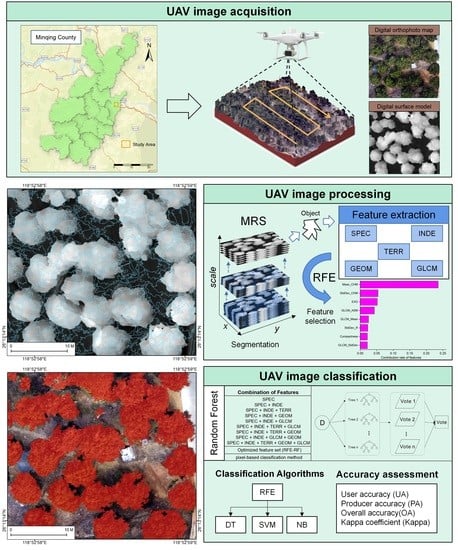
2.1. Study Area

The study area (Figure 1) was located in a Chinese olive tree planting area (118°52′E, 26°13′N) in Minqing County, Fujian Province, China. Minqing County has a subtropical monsoon climate and an altitude of approximately 50 to 140 m; it is located in the eastern part of Fujian Province and the middle and lower reaches of the Minjiang River [36]. The climate in this area is warm and humid with sufficient sunshine and rainfall. The average annual sunshine duration is 1700–2000 h, the average annual temperature is 15–25 °C, the average annual precipitation is 880–2200 mm, and the frost-free period is 230–300 days, which are suitable for the growth of Chinese olive trees. Currently, the planting area of Chinese olive trees in this county is approximately 30 km². The land cover types in the study area mainly included Chinese olive trees, roads, bare land, and grassland, with Chinese olive trees as the main land cover type. The weather was cloudless and rainless during the image acquisition period, and the light conditions were good. The extracted COTCs showed obvious spectral characteristics and textural differences. Therefore, it was suitable for low-altitude UAV flights to collect RS images in the study area during this period.

2.2. UAV Image Acquisition and Pre-Processing

2.2.1. Data Acquisition

The UAV model used for image collection in the study area was DJI Phantom 4 Multi-spectral, which had six complementary metal oxide semiconductors (CMOS) image sensors (1/2.9-inch), including one RGB sensor and five multi-spectral sensors. The effective pixels of a single sensor were 2.08 million. Here, only the RGB sensor of the UAV model was used to obtain images of the study area. The specific parameters of the UAV model are presented (

Table 1. Parameters of DJI Phantom 4 PRO.

UAV Model Wheelbase Weight Max Ascent Speed Max Flight Speed Max Flight Time Hover Accuracy Positioning Module

Phantom 4 Multi-spectral 350 mm 1487 g 6 m/s (Sport Mode), 5 m/s (Manual Mode) 72 km/h (Sport Mode), 50 km/h (Position Mode) 27 min Vertical: ±0.5 m, Horizontal: ±1.5 m GPS + BeiDou + Galileo

). The image collection period was noon in August 2021, and the DJI GS PRO software (DJI Technology Co., Ltd., Shenzhen, China) [5] was used for flight control and route planning. According to the actual conditions of the survey area, the aerial photography parameters were set at 60 m altitude and an 80% overlap between the heading and sideways. In photogrammetry, the structure from motion (SFM) algorithm is one of the most popular algorithms for 3D reconstruction of UAV images. The SFM mainly includes feature point extraction, matching, and geometric verification. It can obtain images at different angles from overlapping images and camera parameters by camera calibration, and then build 3D point cloud models. This study used the Pix4Dmapper software developed by Pix4D (Prilly, Switzerland) [37] to process UAV images, which used an SFM-based algorithm to recover the geometry of a 3D scene from images. The UAV data were reconstructed in 3D to generate DOMs with a resolution of 0.037 m, and DSMs with a resolution of 0.074 m.

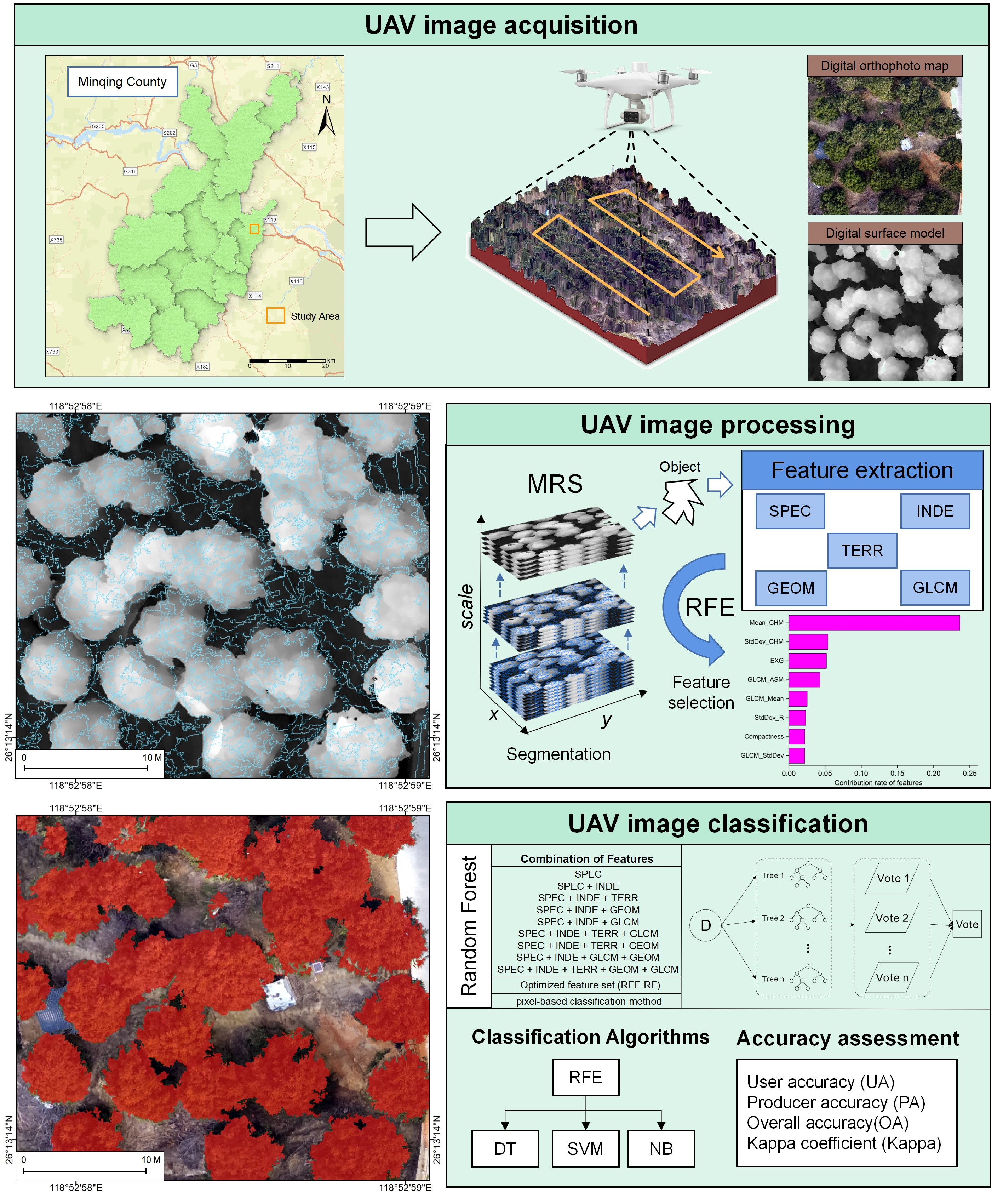
2.2.2. UAV Image Segmentation

Image segmentation is the basis of OBIA technology, and the heterogeneity of segmented image objects is controlled by scale parameters. Therefore, the key to image segmentation lies in the selection of segmentation scale. Here, we used a quantitative method for unsupervised evaluation of segmentation scale and established a mathematical model according to the characteristics of the segmented object. The estimation of scale parameter (ESP) is a tool to measure the homogeneity of pixels in an area by calculating the local variance (LV) and LV rate of change (Equation (1)). The image is segmented by bottom-up iterative multi-scale segmentation, and the optimal segmentation scale is obtained when the LV rate of change (ROC) is the largest, i.e., the peak of ROC [38]:

$$\mathrm{ROC}=\left[\frac{\mathrm{L}-(\mathrm{L}-1)}{\mathrm{L}-1}\right]\times 100$$

(1)

where L is the mean LV in the segmentation result at target level, and L − 1 is the mean LV in the segmentation result at next lower level.

We used the ESP2 plug-in in eCognition Developer 9.0 software (Trimble Germany GmbH, Munich, Germany) [39] to select the optimal segmentation scale for the image and set the weight of each layer to 1. The spectral information of the image is dominant in the RS image and influence of the shape factor parameter is largely controlled by segmentation quality. Therefore, the weight of the spectral information should be given priority when assigning the weight of the spectrum and shape factor. By setting different parameters for multiple testing, we set the weight of the shape factor (shape) and spectral factor (spectrum) to 0.1 and 0.5, respectively. The optimal scale was extracted according to the LV and ROC values under different scale parameters. Figure 2 shows that the LV increases, and ROC decreases with the increase of segmentation scale. To obtain the critical value between over- and under-segmentation of the image, the scale when the ROC curve peaks was selected as the better one. Since there were multiple values for the optimal scale, we took several potential optimal scales such as 20, 38, 55, 68, 86, and 120 when the ROC was at its peak, to segment the image layers.

For the RS images of the study area, we selected several of the above scales when the ROC was at the peak as the scale parameters for segmentation. Figure 3 shows the effects of over-segmentation, optimal segmentation, and under-segmentation scale appearing in the study area. Because of the complexity of ground objects in the study area, the phenomenon of under-segmentation was obvious when the segmentation scale was large. Different types of ground objects were included in the same object, resulting in confusion among the segmentation objects, and the COTC could not be effectively segmented from imagery (Figure 3a). If the segmentation scale is too small, it will be over-segmented, and the segmentation between continuous objects of the same type will be too fragmented (Figure 3c); this will affect the classification accuracy and model training time. After visual interpretation, when the segmentation scale was 68, there was a relatively satisfactory boundary between the tree crown and other ground object categories, and there were fewer objects that were too fragmented in the single tree crown layer (see Figure 3b); thus, the segmentation effect was better. Therefore, we selected 68 as the segmentation scale.

2.3. Crown Feature Extraction and Selection

2.3.1. Crown Elevation Information Extraction

Tree height is an important parameter of single tree structure. With the development of computer vision technology, it is possible to extract single tree structural parameters (tree height) using UAVs. The canopy height model (CHM), which can eliminate the effect of terrain relief on the elevation of ground objects in DSM images, has been widely used to quantify tree heights in UAV images [40]. Here, we used ArcGIS 10.5 software (ESRI Inc., Redlands, CA, USA) to extract the CHM from DSM data. First, we manually identified non-COTC areas in the DSM imagery by visual inspection and created point features. Simultaneously, we imported the elevation values of non-COTC areas into point feature fields. Second, spatial interpolation methods such as inverse distance weighted interpolation, kriging interpolation, natural neighbor, and spline interpolation were used to spatially interpolate the ground point data. In addition, the kriging interpolation method with a better effect was screened through visual interpretation to generate digital terrain models (DTMs). DSM is a model that includes the heights of trees and other objects, reflecting the real surface conditions, whereas the DTM only represents the fluctuation of the terrain without including the elevation values of surface objects. Therefore, the CHM can be generated by performing a difference operation between DSM and DTM (Figure 4).

2.3.2. Crown Segmentation Object Feature Extraction

Spectral features are the basic features of an image and different types of ground objects have different spectral features. Therefore, the differences in spectral information of ground objects in visible band images can be used to distinguish different types of ground objects [41]. HR or UHR RS images contain large volumes of data and usually have complex geometric structures and edge features [42]. Thus, the geometric structural features of the target objects can be used as an effective means of discriminating the types of ground objects. Owing to the unique spectral characteristics of vegetation, different vegetation indices can be obtained through the combined operation of different bands. The vegetation index reflects the vegetation growth status. It has a wide range of applications in forestry to monitor forest destruction, soil erosion, and agricultural monitoring of crop growth, pests, and diseases, as well as in the ecological and environmental fields [43,44,45]. Since visible images lack spectral information in the near-infrared band, the vegetation indices that can be used are limited. To improve the prediction ability of the model and prevent the fitting function from being unable to meet the training set owing to insufficient feature dimensions, it is necessary to provide more features to participate in the training. For example, we improved extraction accuracy by extracting relative elevation features at the single tree scale, and the shape measures consisted of the geometrical features provided by each segmented object. In addition, some studies have shown that texture features extracted by a statistical gray-level co-occurrence matrix (GLCM) can effectively distinguish ground objects with similar spectral features. Based on the above conclusions, we extracted five categories of COTC object features in the study area: spectral (SPEC), geometric (GEOM), and textural (GLCM) features. The corresponding vegetation index (INDE) features were constructed based on the characteristics of the visible spectral image bands, and terrain (TERR) features were constructed based on the relative elevation of the target crown layer. By extracting features and excluding invalid sub-features, we screened out 46 subclass features as follows:

(1)

SPEC: Eight subclass features, i.e., the mean (Mean) and standard deviation (StdDev) of the three bands in the visible image, including the mean of the red band (Mean_R), mean of the green band (Mean_G), mean of the blue band (Mean_B), red band standard deviation (StdDev_R), green band standard deviation (StdDev_G), blue band standard deviation (StdDev_B), band maximum difference (Max_diff), and brightness.

(2)

INDE: Seven vegetation index subclass features (Table 2), i.e., excess green index (EXG), excess red index (EXR), modified green-red vegetation index (MGRVI), red-green-blue vegetation index (RGBVI), normalized green-blue difference index (NGBDI), normalized green-red difference index (NGRDI), and excess green minus excess red (EXGR).

(3)

GLCM: Twelve subclass features for a total of seven texture factors are listed (Table 3). It contains the mean, entropy, angular second moment (ASM), and contrast of the GLCM and gray-level difference vector (GLDV), as well as the correlation, dissimilarity, and homogeneity of the GLCM in all directions.

(4)

GEOM: 17 subclass features, i.e., border index, border length, area, volume, width, length, length/width, compactness, shape index, density, roundness, asymmetry, number of pixels, ellipse fitting, rectangle fitting, radius of largest enclosing ellipse, and radius of smallest enclosing ellipse.

(5)

TERR: Two subclass features, i.e., the mean (Mean_CHM) and standard deviation (StdDev_CHM) of the relative crown elevation (presented in Equation (2)).

Table 2. Seven vegetation index features and corresponding equations (R, G, and B represent the mean value of red, green, and blue bands).

Vegetation Index	Full Name	Equation	Reference
EXG	excess green index	2G − R − B	[46]
EXR	excess red index	1.4R − G	[47]
MGRVI	modified green-red vegetation index	(G2 − R2)/(G2 + R2)	[48]
RGBVI	red-green-blue vegetation index	(G2 − BR)/(G2 + BR)	[49]
NGBDI	normalized green-blue difference index	(G − B)/(G + B)	[50]
NGRDI	normalized green-red difference index	(G − R)/(G + R)	[51]
EXGR	excess green minus excess red	2G − R − B − (1.4R − G)	[52]

Table 2. Seven vegetation index features and corresponding equations (R, G, and B represent the mean value of red, green, and blue bands).

Vegetation Index	Full Name	Equation	Reference
EXG	excess green index	2G − R − B	[46]
EXR	excess red index	1.4R − G	[47]
MGRVI	modified green-red vegetation index	(G2 − R2)/(G2 + R2)	[48]
RGBVI	red-green-blue vegetation index	(G2 − BR)/(G2 + BR)	[49]
NGBDI	normalized green-blue difference index	(G − B)/(G + B)	[50]
NGRDI	normalized green-red difference index	(G − R)/(G + R)	[51]
EXGR	excess green minus excess red	2G − R − B − (1.4R − G)	[52]

Table 3. Seven texture factors and corresponding equations (N: order of GLCM, μ: mean, σ: standard deviation, P_i,j: (i,j)th entry in the GLCM).

Texture Feature	Equation	Reference
Mean	${\displaystyle \sum _{i=1}^N{\displaystyle \sum _{j=1}^{N}i{P}_{i,j}}}$	[53]
Homogeneity	${\displaystyle \sum _{i=1}^N{\displaystyle \sum _{j=1}^N{P}_{i,j}}}/(1+{(i-j)}^2)$	[54]
Contrast	${\displaystyle \sum _{i=1}^N{\displaystyle \sum _{j=1}^N{(i-j)}^2{P}_{i,j}}}$	[55]
Dissimilarity	${\displaystyle \sum _{i=1}^N{\displaystyle \sum _{j=1}^{N}i\underset{i,j}{P}}}|i-j|$	[55]
Entropy	${\displaystyle \sum _{i=1}^N{\displaystyle \sum _{j=1}^N{P}_{i,j}}}\lg P_{i,j}$	[54]
Angular Second Moment	${\displaystyle \sum _{i=1}^N{\displaystyle \sum _{j=1}^{N}i{P}_{i,j}{}^2}}$	[56]
Correlation	$\left[{\displaystyle \sum _{i=1}^N{\displaystyle \sum _{j=1}^{N}ij{P}_{i,j}-{\mu }_1{\mu }_2}}\right]/{\sigma }_1{\sigma }_2$	[54]

Table 3. Seven texture factors and corresponding equations (N: order of GLCM, μ: mean, σ: standard deviation, P_i,j: (i,j)th entry in the GLCM).

Texture Feature	Equation	Reference
Mean	${\displaystyle \sum _{i=1}^N{\displaystyle \sum _{j=1}^{N}i{P}_{i,j}}}$	[53]
Homogeneity	${\displaystyle \sum _{i=1}^N{\displaystyle \sum _{j=1}^N{P}_{i,j}}}/(1+{(i-j)}^2)$	[54]
Contrast	${\displaystyle \sum _{i=1}^N{\displaystyle \sum _{j=1}^N{(i-j)}^2{P}_{i,j}}}$	[55]
Dissimilarity	${\displaystyle \sum _{i=1}^N{\displaystyle \sum _{j=1}^{N}i\underset{i,j}{P}}}|i-j|$	[55]
Entropy	${\displaystyle \sum _{i=1}^N{\displaystyle \sum _{j=1}^N{P}_{i,j}}}\lg P_{i,j}$	[54]
Angular Second Moment	${\displaystyle \sum _{i=1}^N{\displaystyle \sum _{j=1}^{N}i{P}_{i,j}{}^2}}$	[56]
Correlation	$\left[{\displaystyle \sum _{i=1}^N{\displaystyle \sum _{j=1}^{N}ij{P}_{i,j}-{\mu }_1{\mu }_2}}\right]/{\sigma }_1{\sigma }_2$	[54]

2.4. RF Parameter Configuration and Feature Selection

2.4.1. RF Model Introduction

RF is a classifier that integrates multiple decision trees for prediction; Figure 5 shows a conceptual diagram of the RF model. It uses bagging to vote on classification results of several weak classifiers and uses the category with the most votes as the final output to form a strong classifier. It has the advantages of high accuracy, running on large datasets, processing samples with high-dimensional features, and good robustness when dealing with noisy data [57]. The two most important parameters in the RF model include the number of features contained in each tree node (Mtry) and number of decision trees (Ntree), which together determine the classification effect of the model. RF uses a bootstrap sample when constructing each tree, and approximately 1/3 of the samples of each tree do not participate in the training of the model. Such samples are called out-of-bag (OOB) and can be used to calculate feature importance and selection, as well as participate in internal cross-validation to assess the performance of the RF model. The errors generated by these samples are called OOB error rates [58].

2.4.2. RF Parameter Configuration

Here, we constructed the changes in OOB-error when Ntree is from 1 to 1000 under nine different feature combination schemes (see Figure 6). Due to the robustness of the RF model and absence of overfitting, Ntree could be set as large as possible. Considering the computational efficiency of the RF model, we set Ntree to 400 for all schemes according to the OOB error-Ntree curve because beyond this value the OOB error was insensitive to changes in Ntree. Since RF needs to calculate the information gain of all feature contributions of each decision tree node [58], to ensure calculation efficiency, we set Mtry as the square root of the number of input features.

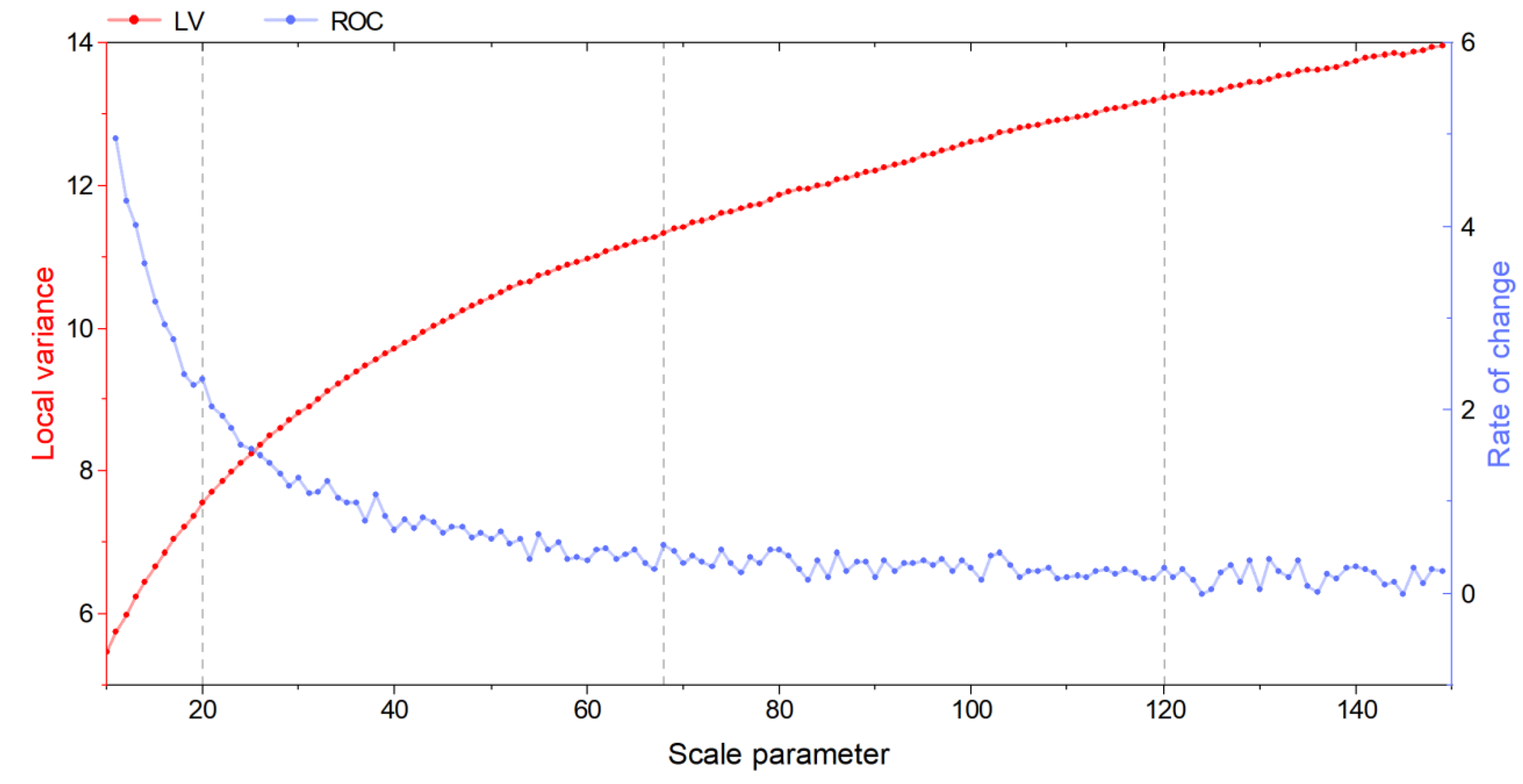
2.4.3. Feature Optimization

To determine the optimal number of features in the RF model, we used recursive feature elimination (RFE) for feature optimization. First, we input all features in the object as initial features into the classifier and used the OOB samples generated by the RF model for cross-validation to obtain the prediction accuracy of the classifier in this feature combination; then, the importance of each feature was obtained [59]. Second, the feature with the lowest feature importance is removed from the original feature set each time, and the new feature subset is input to the classifier. Through the continuous loop iteration of the above method, the prediction accuracy of 46 sets of feature subsets was obtained (Figure 7a). The figure shows that the prediction accuracy increased rapidly with the input of features with higher importance scores, and the local maximum point of the prediction accuracy appeared when the number of features was eight. Subsequently, the prediction accuracy decreased with an increase in the number of features until the input of the 13th feature started to increase slowly. To improve the classification efficiency, we selected as few feature subsets as possible as the optimal feature combination to participate in the training of the model under the premise of ensuring prediction accuracy. Based on the feature importance ranking (Figure 7b), we retained a total of eight feature indices, including Mean_CHM, StdDev_CHM, EXG, GLCM_ASM, GLCM_Mean, StdDev_R, Compactness, and GLCM_StdDev. The above indices cover five categories of features: spectrum, vegetation index, shape, texture, and terrain.

2.5. Research Scheme Design

Here, the experimental scheme (

Table 4. Design of experimental schemes.

Classification Method	Scheme	Classification Algorithms	Combination of Features	Number of Features
Object-based image analysis	S1	Random Forest	SPEC	8
	S2		SPEC + INDE	15
	S3		SPEC + INDE + TERR	17
	S4		SPEC + INDE + GEOM	32
	S5		SPEC + INDE + GLCM	27
	S6		SPEC + INDE + TERR + GLCM	29
	S7		SPEC + INDE + TERR + GEOM	34
	S8		SPEC + INDE + GLCM + GEOM	44
	S9		SPEC + INDE + TERR + GEOM + GLCM	46
Object-based image analysis	S10	Random Forest	Mean_CHM, SD_CHM, EXG, Angular second moment, Mean_GLCM, SD_R, Compactness SD_GLCM	8
	S11	Decision Tree	Mean_CHM, SD_CHM, EXG, Angular second moment, Mean_GLCM, SD_R, Compactness SD_GLCM	8
	S12	Support Vector Machine	Mean_CHM, SD_CHM, EXG, Angular second moment, Mean_GLCM, SD_R, Compactness SD_GLCM	8
	S13	Naive Bayesian	Mean_CHM, SD_CHM, EXG, Angular second moment, Mean_GLCM, SD_R, Compactness SD_GLCM	8
Pixel-based classification	S14	Random Forest	SPEC, EXG, CHM	5

) was designed based on the spectral features of visible images, RF algorithm, and five different feature types of vegetation index, texture, geometry, and terrain of image objects in the study area. The research scheme was designed based on the following three research objectives:

(1)

To study the results of different feature combination schemes for COTC extraction. First, the spectral features of visible images were taken as the first scheme (S1). Second, since the vegetation index was the most commonly used feature that could effectively distinguish between different vegetation types, as well as between vegetation and other ground object types [60], the spectral and constructed vegetation index features were used as the second scheme (S2). The remaining three feature types were added in sequence in the form of arrangements and combinations, and nine experimental schemes (S1–S9) were constructed.

(2)

To study the extraction effect of different algorithms on COTC and assess the extraction accuracy after feature dimensionality reduction. The top eight features ranked by importance were selected as the features of the selected samples; RF, DT, SVM, and NB—four commonly used ML classifiers—were used for training to construct schemes S10–S13.

(3)

To compare the effects of the single PB classification and multi-feature fusion OBIA methods on COTC extraction. Based on the RF algorithm, we compared the OBIA and traditional PB classification methods to construct scheme S14.

2.6. Selecting Sample Point and Evaluating Accuracy

2.6.1. Selecting Study Area Sample

To reduce the interference of mixed pixels and accurately extract the Chinese olive crown layer from images, we considered the land cover types in the study area and grouped COTC as the main type into one category. Meanwhile, other features, such as grass, bare land, and roads, were grouped into another category for binary classification. We selected homogeneous, random, and representative samples and ensured that the sample points were built on objects that contained only a single land cover type [61]. First, we scaled the image into 3 × 3 subplots to ensure that the test points were evenly distributed over the image. Second, we randomly generated sufficient number of sample points (2000 in total) using ArcGIS 10.5 (ESRI Inc., Redlands, CA, USA) [62] to ensure that each subplot had enough sample points, and then we randomly selected 400 (179 in COTC and 221 in Non-COTC) as the test points for evaluating accuracy. Among the remaining 1600 points, the sample points established on the non-COTC were removed individually in nine subplots through visual interpretation, to ensure that the training samples were the objects established on the COTC and are not duplicated with the test points. Finally, the filtered 600 COTC samples were retained as training sample points.

2.6.2. Accuracy Evaluation Index

Here, we selected 400 points (179 in COTC, 221 in non-COTC) for accuracy evaluation, and added the value (0 was non-COTC, 1 was COTC) of the actual category of the surface to the attribute table of each test point after visual interpretation and field verification. Simultaneously, the results of binary classification were extracted to the attribute table of test points according to the same category number to construct a confusion matrix. Confusion matrices are commonly used in supervised learning to evaluate algorithm performance and present visualized classification results [63]. The evaluation indicators included user accuracy (UA) (presented in Equation (2)) [64], producer accuracy (PA) (presented in Equation (3)) [64], overall accuracy (OA) (presented in Equation (4)) [65], and kappa coefficient (Kappa) (presented in Equation (5)) [65]. The UA is the proportion of the number of correctly classified test points in the category to the number of true surface-type test points. The PA is the proportion of correctly classified test points in the category to the number of test points in the category defined by the classifier. The OA is the proportion of correctly classified test points to the total number of test points. In addition, the Kappa considers the balance between the number of samples in each category and overall accuracy and is often used for classification model accuracy assessment:

$$\mathrm{User}\mathrm{accuracy}=\frac{N_{kk}}{N_{k+}}\times 100\%$$

(2)

$$\mathrm{Producer}\mathrm{accuracy}=\frac{N_{kk}}{N_{+k}}\times 100\%$$

(3)

$$\mathrm{Overall}\mathrm{accuracy}=\frac{{\displaystyle {\sum }_{k=1}^2{N}_{kk}}}{N_{total}}\times 100\%$$

(4)

$$\mathrm{Kappa}\mathrm{coefficient}=\frac{N_{total}{\displaystyle {\sum }_{k=1}^2{N}_{kk}-{\displaystyle {\sum }_{k=1}^2{N}_{k+}{N}_{+k}}}}{N_{total}-{\displaystyle {\sum }_{k=1}^2{N}_{k+}{N}_{+k}}}$$

(5)

where N_total is the total number of test points, N_kk is the number of test points correctly classified into k type, N_k+ is the total number of test points of k type in the classification image, and N_+k is the total number of test points of k type on the real surface (k = 1 represents COTC, k = 2 represents non-COTC).

3. Results

3.1. Accuracy Evaluation of Different Feature Combination Schemes

The binary classification extraction results of COTC with different feature dimension schemes based on OBIA-RF are shown (Figure 8). The RGB true color composite image of the local image in the study area is shown (Figure 8a). The training samples were extracted using only spectral features (Figure 8b). There were serious misclassifications and omissions in the picture, and many herbaceous plants were incorrectly classified as Chinese olive trees. This may be because the color of herbaceous plants was greenish, and the spectral features were close to those of the COTC. Simultaneously, some darker areas in the COTC were missed in the classification because of the influence of the incident angle of sunlight and shading of leaves. Vegetation index features were added based on spectral features, as Figure 8c shows, and the extraction effect was greatly improved. However, because the visible band had fewer vegetation indices than multispectral sensors with near-infrared band, the COTC was easily misclassified into other vegetation types with similar spectral features, such as single-growing shrubs. Therefore, we successively introduced geometric and textural features (Figure 8d,e). The extraction results were less different, and the addition of textural and geometric features could improve the accuracy of identifying non-COTC shadow areas. However, it was difficult to improve the misclassification phenomenon between different vegetation types. After adding terrain features, the extraction results of the scheme based on all features are shown (Figure 8f). In comparison with previous schemes, the misclassification of different vegetation types and omission of crown contours and shadow areas were improved. Based on visual assessment and the verification results of the test points, it was concluded that the extraction results of this scheme were the closest to the actual situation in the study area.

To quantitatively describe the extraction accuracy of the RF algorithm in the OBIA method for dealing with the binary classification problem, we calculated the quantitative evaluation indicators (UA and PA of the target object type, and OA and Kappa of the overall classification result). Simultaneously, we divided the extraction results of the image objects where the accuracy verification points were located into true positive (TP), false positive (FP), true negative (TN), and false negative (FN) (the sum of the above four points was the total number of accuracy verification points). The COTC extraction results were analyzed using a RF algorithm based on different and optimal feature combinations (Figure 9).

From the numerical relationship, in all schemes, the overall accuracy was between 85.75% and 97%, and the Kappa coefficient was between 0.71 and 0.94. This showed that the combination of the OBIA and RF algorithms could obtain high accuracy in the binary classification of HR images. Among all schemes, S1 only used spectral features of the image to extract target objects, and the overall accuracy and Kappa coefficient were the lowest at 85.75% and 0.71, respectively. The extraction accuracy was significantly improved after the vegetation index feature was added to S2, and the overall accuracy and Kappa coefficient increased by 9% and 0.18, respectively; this indicates that the vegetation index was effective in the extraction of COTC, and the increase in the feature dimensionality had a positive effect on extraction accuracy. To clarify the influence of feature dimensionality on extraction accuracy, terrain, geometric, and textural features were added to the S3–S5 schemes, respectively, and all three schemes improved their extraction accuracy. Among them, terrain features had the greatest improvement in OA and Kappa, whereas geometric and textural features had similar contribution rates to extraction accuracy and were both less than terrain features. Therefore, the extraction accuracy was not only related to the number of features, but to the contribution rate of different feature types to the extraction accuracy of target ground objects. To prove the above conclusion, the three features of terrain, geometry, and texture were combined in pairs, and the spectral and vegetation index features were added to construct schemes S6–S8; in comparison with the first five schemes S1–S5, the accuracy of the three schemes was improved. The classification accuracy of scheme S8 was higher than that of S4 and S5 after introducing geometric and textural features, but less than that of schemes S6 and S7 with terrain features. It could be seen that the extraction accuracy of COTC generally increased with the increase of number of features, but it was related to the contribution rate of different feature types to the extraction accuracy. To obtain the highest accuracy, all feature categories that have a positive contribution to the extraction accuracy were used to construct scheme S9; through the accuracy evaluation, the OA and Kappa were 97.00% and 0.94, respectively, and the extraction accuracy was the highest among all schemes, which proved the above conclusion. Among all features with positive contribution rates, redundant features contributed less to the extraction accuracy. Therefore, we constructed scheme S10 by extracting the top eight features with the highest importance after dimensionality reduction of all features. The OA and Kappa of S10 were 96.50% and 0.93, respectively, which were only 0.50% and 0.01 different from those obtained using all 46 features, and the classification accuracy using the optimized features reached 99% of the accuracy achieved using all features. The above conclusions show that it was not necessary to extract all features of the target ground objects when participating in the model training. Simultaneously, it indicated that the RF algorithm could not only deal with high-dimensional features but showed good performance in lower-dimensional features.

The producer and user accuracies of COTC extraction in schemes S1–S10 were compared (Figure 10). For S1, constructed with only spectral features, the UA and PA in extracting COTCs were both 83.52% and 84.92%, respectively; i.e., the lowest among all schemes. This shows that relying only on spectral features to extract COTC would lead to higher misclassification and missed classification errors, which was reflected in the lower UA and PA. For S2, once the vegetation index features were added, the commission error (CE) and omission error (OE) were reduced. In the follow-up schemes, S3 to S10, both CE and OE were controlled within approximately 5%. Among them, the CE of S3 and OE of S6 and S7 showed lower values in all schemes. The scheme with the lowest CE was S7 and S9, the error was 3.35%, and the scheme with the lowest OE was S10 (all of the above schemes contain terrain features). The above data showed that the terrain features could significantly reduce CE and OE and improve extraction accuracy when extracting the Chinese olive canopy. This might be due to the obvious height difference between Chinese olive trees and other features in the image, and terrain features could avoid the effects of noise in visible RS images.

3.2. Accuracy Evaluation of Different Classification Algorithms

Here, we compared the differences in accuracy of COTC extraction between different classification methods and commonly used ML methods, since the optimized feature set could achieve high accuracy in the RF model. Therefore, according to the contribution rate of the classification accuracy of each feature to the importance of the RF model, the feature subset with the top eight importance after optimization was selected as the feature index for evaluating the performance of each classifier. In the eCognition 9.0 software, the RF algorithm and traditional ML algorithms, such as DT, NB, SVM, and PB classification methods, were used to extract target objects, and the extraction accuracy of each algorithm was compared. Different classifiers require adjustment of different parameters. To determine the optimal parameters, we manually adjusted a series of values of the parameters required by different algorithms, performed accuracy verification, and used the parameter configuration with the highest extraction accuracy as the extraction result of this classifier. The extraction results of different algorithms are shown (Figure 11). It can be seen intuitively from the figure that the RF algorithm in OBIA was significantly better than the other algorithms in extracting COTC (Figure 11a). OBIA-RF had high recognition accuracy for COTC and high consistency with the distribution of real ground objects, which indicated that RF had the highest adaptability for COTC extraction compared with other algorithms. In comparison with the OBIA-RF extraction results, other algorithms had higher CE and OE. Among them, the DT algorithm had the worst extraction effect, which was mainly reflected in the incomplete extraction of the continuous crown surface. However, the extraction effect of the DT algorithm between different ground objects was better than that of the SVM (Figure 11b,c). This is because a single decision tree has poor generalization ability, cannot predict data well, and is prone to overfitting when dealing with large datasets [66]. Furthermore, NB is a high-bias, low-variance classifier and is a relatively simple generative model [67]; its extraction effect was only second to RF (Figure 11d). This shows that the NB algorithm performs well on small-scale datasets. To demonstrate the superiority of the OBIA method, the RF algorithm with the best performance on the optimized feature set was used to compare the extraction results of the traditional PB classification method under the same parameter configuration (Figure 11e). It can be seen from the figure that the size of the target COTC obviously exceeded the actual range, and there was a lot of salt-and-pepper noise.

A quantitative analysis of the UA and PA of Chinese olive trees from the confusion matrix of the extraction results of different algorithms (

Table 5. Confusion matrix of extraction results of different algorithms.

(a)	Class value	Other	COTC	Total	UA/%	(b)	Class value	Other	COTC	Total	UA/%
	Other	218	11	229	95.20		Other	219	29	248	88.31
	COTC	3	168	171	98.25		COTC	2	150	152	98.68
	Total	221	179	400			Total	221	179	400
	PA/%	98.64	93.85				PA/%	99.10	83.80
(c)	Class value	Other	COTC	Total	UA/%	(d)	Class value	Other	COTC	Total	UA/%
	Other	209	18	227	92.07		Other	218	17	235	92.77
	COTC	12	161	173	93.06		COTC	3	162	165	98.18
	Total	221	179	400			Total	221	179	400
	PA/%	94.57	89.94				PA/%	98.64	90.50
(e)	Class value	Other	COTC	Total	UA/%
	Other	204	1	205	99.51
	COTC	17	178	195	91.28
	Total	221	179	400
	PA/%	92.31	99.44

UA and PA represent user accuracy and producer accuracy. Total represents the total number of test points in row or column. COTC represents Chinese olive tree crown.

). The algorithm with the highest CE was the PB classification method, and the misclassification rate reached 7.69%. This might be because binary extraction was performed in RS images with complex ground object types, and there were a large number of mixed pixels in other ground types. This resulted in a much lower number of samples of objects with different spectral information than that of the target objects. The performance was that the UA of the target feature was low, and the misclassification was serious. The OBIA-RF algorithm had lower CE and OE (1.75% and 6.15%, respectively), which was the best among all algorithms.

A quantitative analysis of the extraction accuracy of different algorithms in the optimized feature set in terms of the numerical relationship between the OA and Kappa is shown (

Table 6. Comparison of accuracy of different classification algorithms for COTC extraction.

Scheme	Classification Methods	Classification Algorithms	Overall Accuracy/%	Kappa Coefficient	Time Used/s
S10	Object-based image analysis	Random Forest	96.50%	0.93	358
S11		Decision Tree	92.25%	0.84	362
S12		Support Vector Machine	92.50%	0.85	761
S13		Naive Bayesian	95.00%	0.90	351
S14	Pixel-based classification	Random Forest	95.50%	0.91	205

). The data in the table show that the RF algorithm had the highest extraction accuracy in OBIA, and the OA and Kappa coefficient were 96.50% and 0.93, respectively. The OA and Kappa of the PB classification method were 95.50% and 0.91, respectively, which were higher than the extraction results of the DT, SVM, and NB classifiers. The algorithm with the lowest extraction accuracy was DT, with OA and Kappa values of 92.25% and 0.84, respectively. This might be due to the fact that a single decision tree was prone to overfitting when dealing with out-of-sample datasets compared with an RF composed of multiple decision trees; thus, it was more prone to misclassification. Simultaneously, in the same RF algorithm, the overall extraction accuracy of the OBIA method was higher than that of the PB classification method. Moreover, the accuracy evaluation method based on random point verification made it difficult to detect the accuracy loss caused by the noise phenomenon in the PB classification method. Therefore, the actual classification accuracy and precision of the PB classification method were lower than those of the data in the table. The following conclusions were drawn from the data:

(1)

In addition, the RF algorithm can obtain high-precision classification results when dealing with a feature set after dimensionality reduction.

(2)

The OBIA method can describe the attributes of ground objects more accurately, and the extraction accuracy is higher because the object entity has a more complex shape, texture, and other features and spatial relationships than a single pixel.

Therefore, the combination of the OBIA and RF algorithms showed better performance in COTC extraction.

4. Discussion

To improve the investigating methods for forestry, this study used Chinese olive trees in a broad-leaved tree species widely distributed in China as the research object. Owing to the high acquisition cost of traditional earth observation satellites and the fact that they are significantly affected by weather conditions, it is difficult to ensure the accuracy and time continuity of satellite RS platforms. UAVs have been increasingly used in the field of RS because of their ability to acquire HR images under cloudy conditions and low difficulty of acquisition. With advancements in the automation capabilities of UAVs, they are widely used in various fields, such as resource detection, geographic mapping, and disaster monitoring. Owing to the low flying height, high resolution of UAVs, and the complexity of ground object types, the amount of RS data and the difficulty of data processing have increased significantly. In recent years, ML algorithms have emerged as automated and intelligent algorithms, meeting the needs of massive RS data processing and compensating for the low efficiency of image processing in the OBIA method. In view of this, we used consumer-grade UAVs to achieve precise extraction of COTC at the single tree scale, thereby reducing labor costs and improving efficiency. The novelty of this study is that the COTC parameters were obtained in the visible band. The OA of all schemes formulated using the binary classification model was above 85.75%. We divided other ground objects into the same category, except for Chinese olive trees. In comparison with multi-classification models in most studies, the binary classification model could increase the feature differences between Chinese olive trees and other ground objects so that the classifier could distinguish different ground objects more effectively. We used an estimation of scale parameter (ESP) to control the degree of image object heterogeneity to extract high-quality geometric and texture features from HR image objects. There are complex types of ground objects in the Chinese olive grove, which makes it difficult to obtain the parameters of the target tree species with high precision. With continuous improvement of the spatial resolution of RS images, in areas with large spatial heterogeneity, the similar spectral features between different objects greatly increase the difficulty of extracting the target ground objects. Since the traditional PB classification method has difficulty performing multi-feature fusion on training samples, this study used the OBIA method. The OBIA method can use the texture, geometry, and spatial relationship features of segmented objects, which greatly improved the extraction accuracy of COTC. To eliminate the redundancy of features and improve extraction efficiency, we used OOB samples to analyze the importance of different features and used RFE to screen features. We used the optimized features to compare the performance of RF with other ML algorithms (DT, SVM, NB, and PB) to check the accuracy and time consumption of different models.

RF classifiers in RS have been successfully applied to flood risk mapping [68], assessing carbon stocks in the topsoil [69], and combined with UAV imagery to estimate yield [70]. Many studies compared RF to other mainstream ML classifiers, demonstrating that the classification accuracy of the RF algorithm was better than that of the DT and Bayes classifier [71]. However, in terms of execution time, classifiers such as DT are superior to RF [72]. Adugna et al. [73] suggested that the performance of RF was comparable to that of SVM in classifying images with less mixed pixels. However, RF was more efficient than SVM when dealing with high-dimensional features or high-dimensional input data. In addition, because the performance of SVM depends on parameter setting and feature selection, it was less effective when dealing with large datasets. Therefore, SVM was less applicable than RF [74]. Although RF has the ability to manage high-dimensional features and achieve high accuracy with default parameters, we optimized its two most important parameters (Ntree and Mtry) so that the RF model could achieve better classifying results and increased executing speed. Currently, there are some studies on OBIA combined with RF [32,75,76,77]. Wang et al. [32] achieved high-precision classification at single tree scale in urban forests by extracting multiple features such as spectrum and texture, with an OA of 91.3%. However, their study did not address the redundancy of high-dimensional features. In our study, a recursive feature elimination method (RFE) was used to eliminate features with less correlation, which improved computational efficiency. Li et al. [77] combined OBIA and different models to classify shrub individuals, and compared the classification accuracy of the different models combined with different features. The results showed that combining the optimal feature set and RF model could obtain the best classification accuracy, with an OA of 88.63%. However, there was no quantitative index to select the optimal scale for segmenting images and did not introduce the geometric features of the object in this study. Our study used the ESP tool to quantitatively screen segmentation parameters. In addition, we used the SFM algorithm to reconstruct 3D points; then, we obtained the tree height parameter as an input feature for the classifier, which was the highest in all feature importance ranking.

Based on the above discussions, our improvement to the OBIA-RF algorithm has broad application prospects for the precise management of forestry. With the increased use of UAVs in the field of RS and emergence of more advanced and effective algorithms such as convolutional neural networks and transformers, our method could be used in forestry surveys, including single tree parameter extraction and monitoring of physiological conditions. Ultimately, automation, informatization, and precision forestry resource management will be realized, and sustainable development of forestry could be promoted.

5. Conclusions

The following conclusions were drawn from our study:

First, the RF algorithm achieved high accuracy in processing high- and low-dimensional features, and the OA of all schemes was above 85.75% and up to 97.00%. This indicates that the RF algorithm can achieve ideal results in the extraction of crown-width parameters. Second, an increase in feature dimensionality can improve the extraction accuracy of COTC, and fewer features can affect the classification accuracy of the model when dealing with large datasets. With an increase in feature dimensionality, the model extraction accuracy of the crown continuously improved. In comparison with the scheme using only spectral features, the OA of the scheme using all features was improved by 11.25%, and the Kappa coefficient was increased by 0.22; this was a significant improvement in model accuracy. Third, among all features, there were noise features that contributed less or had a negative impact on model accuracy; this might have caused the RF model to produce a certain degree of generalization error. To this end, we used an encapsulated feature selection method, i.e., RFE, to eliminate irrelevant features and retained a total of eight feature subclasses after screening. The OA was only 0.50% different from when all features were used, and the classification efficiency was significantly improved, while ensuring the performance of the model. Lastly, in comparison with other ML algorithms (i.e., DT, SVM, and NB), the OBIA-RF algorithm achieved the highest accuracy under the optimized feature set, and the OA and Kappa were 96.5% and 0.93, respectively. The OBIA-RF model can achieve high accuracy with default parameters, and it has certain advantages in terms of the time consumption of model training.

References

1. Watanabe, Y.; Hinata, K.; Qu, L.; Kitaoka, S.; Watanabe, M.; Kitao, M.; Koike, T. Effects of Elevated CO2 and Nitrogen Loading on the Defensive Traits of Three Successional Deciduous Broad-Leaved Tree Seedlings. Forests 2021, 12, 939. [Google Scholar] [CrossRef]
2. Yao, L.; Wang, Z.; Zhan, X.; Wu, W.; Jiang, B.; Jiao, J.; Yuan, W.; Zhu, J.; Ding, Y.; Li, T.; et al. Assessment of Species Composition and Community Structure of the Suburban Forest in Hangzhou, Eastern China. Sustainability 2022, 14, 4304. [Google Scholar] [CrossRef]
3. Xu, R.; Wang, L.; Zhang, J.; Zhou, J.; Cheng, S.; Tigabu, M.; Ma, X.; Wu, P.; Li, M. Growth Rate and Leaf Functional Traits of Four Broad-Leaved Species Underplanted in Chinese Fir Plantations with Different Tree Density Levels. Forests 2022, 13, 308. [Google Scholar] [CrossRef]
4. Siljeg, A.; Panda, L.; Domazetovic, F.; Maric, I.; Gasparovic, M.; Borisov, M.; Milosevic, R. Comparative Assessment of Pixel and Object-Based Approaches for Mapping of Olive Tree Crowns Based on UAV Multispectral Imagery. Remote Sens. 2022, 14, 757. [Google Scholar] [CrossRef]
5. Ye, Z.; Wei, J.; Lin, Y.; Guo, Q.; Zhang, J.; Zhang, H.; Deng, H.; Yang, K. Extraction of Olive Crown Based on UAV Visible Images and the U2-Net Deep Learning Model. Remote Sens. 2022, 14, 1523. [Google Scholar] [CrossRef]
6. Tian, Y.; Wu, B.; Su, X.; Qi, Y.; Chen, Y.; Min, Z. A Crown Contour Envelope Model of Chinese Fir Based on Random Forest and Mathematical Modeling. Forests 2020, 12, 48. [Google Scholar] [CrossRef]
7. Majasalmi, T.; Rautiainen, M. The impact of tree canopy structure on understory variation in a boreal forest. For. Ecol. Manag. 2020, 466, 118100. [Google Scholar] [CrossRef]
8. Yurtseven, H.; Akgul, M.; Coban, S.; Gulci, S. Determination and accuracy analysis of individual tree crown parameters using UAV based imagery and OBIA techniques. Measurement 2019, 145, 651–664. [Google Scholar] [CrossRef]
9. Ferreira, M.P.; Almeida, D.R.A.d.; Papa, D.d.A.; Minervino, J.B.S.; Veras, H.F.P.; Formighieri, A.; Santos, C.A.N.; Ferreira, M.A.D.; Figueiredo, E.O.; Ferreira, E.J.L. Individual tree detection and species classification of Amazonian palms using UAV images and deep learning. For. Ecol. Manag. 2020, 475, 118397. [Google Scholar] [CrossRef]
10. Dong, T.; Zhang, X.; Ding, Z.; Fan, J. Multi-layered tree crown extraction from LiDAR data using graph-based segmentation. Comput. Electron. Agric. 2020, 170, 105213. [Google Scholar] [CrossRef]
11. Pu, R.; Landry, S. A comparative analysis of high spatial resolution IKONOS and WorldView-2 imagery for mapping urban tree species. Remote Sens. Environ. 2012, 124, 516–533. [Google Scholar] [CrossRef]
12. Jiang, Z.; Wen, Y.; Zhang, G.; Wu, X. Water Information Extraction Based on Multi-Model RF Algorithm and Sentinel-2 Image Data. Sustainability 2022, 14, 3797. [Google Scholar] [CrossRef]
13. Gyawali, A.; Aalto, M.; Peuhkurinen, J.; Villikka, M.; Ranta, T. Comparison of Individual Tree Height Estimated from LiDAR and Digital Aerial Photogrammetry in Young Forests. Sustainability 2022, 14, 3720. [Google Scholar] [CrossRef]
14. Wang, Y.; Xu, X.; Huang, L.; Yang, G.; Fan, L.; Wei, P.; Chen, G. An Improved CASA Model for Estimating Winter Wheat Yield from Remote Sensing Images. Remote Sens. 2019, 11, 1088. [Google Scholar] [CrossRef] [Green Version]
15. Liu, W.; Liu, S.; Zhao, J.; Duan, J.; Chen, Z.; Guo, R.; Chu, J.; Zhang, J.; Li, X.; Liu, J. A remote sensing data management system for sea area usage management in China. Ocean. Coast. Manag. 2018, 152, 163–174. [Google Scholar] [CrossRef]
16. Miraki, M.; Sohrabi, H.; Fatehi, P.; Kneubuehler, M. Individual tree crown delineation from high-resolution UAV images in broadleaf forest. Ecol. Inform. 2021, 61, 101207. [Google Scholar] [CrossRef]
17. Kolanuvada, S.R.; Ilango, K.K. Automatic Extraction of Tree Crown for the Estimation of Biomass from UAV Imagery Using Neural Networks. J. Indian Soc. Remote Sens. 2020, 49, 651–658. [Google Scholar] [CrossRef]
18. Sarabia, R.; Aquino, A.; Ponce, J.M.; López, G.; Andújar, J.M. Automated Identification of Crop Tree Crowns from UAV Multispectral Imagery by Means of Morphological Image Analysis. Remote Sens. 2020, 12, 748. [Google Scholar] [CrossRef] [Green Version]
19. Sarron, J.; Malézieux, É.; Sané, C.; Faye, É. Mango Yield Mapping at the Orchard Scale Based on Tree Structure and Land Cover Assessed by UAV. Remote Sens. 2018, 10, 1900. [Google Scholar] [CrossRef] [Green Version]
20. Ahmadi, P.; Mansor, S.; Farjad, B.; Ghaderpour, E. Unmanned Aerial Vehicle (UAV)-Based Remote Sensing for Early-Stage Detection of Ganoderma. Remote Sens. 2022, 14, 1239. [Google Scholar] [CrossRef]
21. Sharma, P.; Leigh, L.; Chang, J.; Maimaitijiang, M.; Caffe, M. Above-Ground Biomass Estimation in Oats Using UAV Remote Sensing and Machine Learning. Sensors 2022, 22, 601. [Google Scholar] [CrossRef] [PubMed]
22. Aeberli, A.; Johansen, K.; Robson, A.; Lamb, D.W.; Phinn, S. Detection of Banana Plants Using Multi-Temporal Multispectral UAV Imagery. Remote Sens. 2021, 13, 2123. [Google Scholar] [CrossRef]
23. Han, R.; Liu, P.; Wang, G.; Zhang, H.; Wu, X.; Hong, S.-H. Advantage of Combining OBIA and Classifier Ensemble Method for Very High-Resolution Satellite Imagery Classification. J. Sens. 2020, 2020, 1–15. [Google Scholar] [CrossRef]
24. Hossain, M.D.; Chen, D. Segmentation for Object-Based Image Analysis (OBIA): A review of algorithms and challenges from remote sensing perspective. ISPRS J. Photogramm. Remote Sens. 2019, 150, 115–134. [Google Scholar] [CrossRef]
25. Nuijten, R.J.G.; Kooistra, L.; De Deyn, G.B. Using Unmanned Aerial Systems (UAS) and Object-Based Image Analysis (OBIA) for Measuring Plant-Soil Feedback Effects on Crop Productivity. Drones 2019, 3, 54. [Google Scholar] [CrossRef] [Green Version]
26. Belgiu, M.; Csillik, O. Sentinel-2 cropland mapping using pixel-based and object-based time-weighted dynamic time warping analysis. Remote Sens. Environ. 2018, 204, 509–523. [Google Scholar] [CrossRef]
27. Zheng, X.; Wang, Y.; Gan, M.; Zhang, J.; Teng, L.; Wang, K.; Shen, Z.; Zhang, L. Discrimination of Settlement and Industrial Area Using Landscape Metrics in Rural Region. Remote Sens. 2016, 8, 845. [Google Scholar] [CrossRef] [Green Version]
28. Fu, G.; Zhao, H.; Li, C.; Shi, L. Segmentation for High-Resolution Optical Remote Sensing Imagery Using Improved Quadtree and Region Adjacency Graph Technique. Remote Sens. 2013, 5, 3259–3279. [Google Scholar] [CrossRef] [Green Version]
29. Wang, F.; Yang, W.; Ren, J. Adaptive scale selection in multiscale segmentation based on the segmented object complexity of GF-2 satellite image. Arab. J. Geosci. 2019, 12, 699. [Google Scholar] [CrossRef]
30. Phiri, D.; Morgenroth, J.; Xu, C.; Hermosilla, T. Effects of pre-processing methods on Landsat OLI-8 land cover classification using OBIA and random forests classifier. Int. J. Appl. Earth Obs. Geoinf. 2018, 73, 170–178. [Google Scholar] [CrossRef]
31. Luciano, A.C.d.S.; Picoli, M.C.A.; Rocha, J.V.; Duft, D.G.; Lamparelli, R.A.C.; Leal, M.R.L.V.; Le Maire, G. A generalized space-time OBIA classification scheme to map sugarcane areas at regional scale, using Landsat images time-series and the random forest algorithm. Int. J. Appl. Earth Obs. Geoinf. 2019, 80, 127–136. [Google Scholar] [CrossRef]
32. Wang, X.; Wang, Y.; Zhou, C.; Yin, L.; Feng, X. Urban forest monitoring based on multiple features at the single tree scale by UAV. Urban For. Urban Green. 2021, 58, 126958. [Google Scholar] [CrossRef]
33. Zollini, S.; Alicandro, M.; Dominici, D.; Quaresima, R.; Giallonardo, M. UAV Photogrammetry for Concrete Bridge Inspection Using Object-Based Image Analysis (OBIA). Remote Sens. 2020, 12, 3180. [Google Scholar] [CrossRef]
34. Marcial-Pablo, M.d.J.; Ontiveros-Capurata, R.E.; Jiménez-Jiménez, S.I.; Ojeda-Bustamante, W. Maize Crop Coefficient Estimation Based on Spectral Vegetation Indices and Vegetation Cover Fraction Derived from UAV-Based Multispectral Images. Agronomy 2021, 11, 668. [Google Scholar] [CrossRef]
35. Deur, M.; Gašparović, M.; Balenović, I. An Evaluation of Pixel- and Object-Based Tree Species Classification in Mixed Deciduous Forests Using Pansharpened Very High Spatial Resolution Satellite Imagery. Remote Sens. 2021, 13, 1868. [Google Scholar] [CrossRef]
36. Rashid, H.; Yang, K.; Zeng, A.; Ju, S.; Rashid, A.; Guo, F.; Lan, S. The Influence of Landcover and Climate Change on the Hydrology of the Minjiang River Watershed. Water 2021, 13, 3554. [Google Scholar] [CrossRef]
37. Lagogiannis, S.; Dimitriou, E. Discharge Estimation with the Use of Unmanned Aerial Vehicles (UAVs) and Hydraulic Methods in Shallow Rivers. Water 2021, 13, 2808. [Google Scholar] [CrossRef]
38. Lu, H.; Liu, C.; Li, N.; Fu, X.; Li, L. Optimal segmentation scale selection and evaluation of cultivated land objects based on high-resolution remote sensing images with spectral and texture features. Environ. Sci. Pollut. Res. 2021, 28, 27067–27083. [Google Scholar] [CrossRef]
39. Rana, M.; Kharel, S. Feature Extraction for Urban and Agricultural Domains Using Ecognition Developer. Int. Arch. Photogramm. Remote Sens. Spat. Inf. Sci. 2019, XLII-3/W6, 609–615. [Google Scholar] [CrossRef] [Green Version]
40. Zarco-Tejada, P.J.; Diaz-Varela, R.; Angileri, V.; Loudjani, P. Tree height quantification using very high resolution imagery acquired from an unmanned aerial vehicle (UAV) and automatic 3D photo-reconstruction methods. Eur. J. Agron. 2014, 55, 89–99. [Google Scholar] [CrossRef]
41. Zhang, H.; Wang, Y.; Shang, J.; Liu, M.; Li, Q. Investigating the impact of classification features and classifiers on crop mapping performance in heterogeneous agricultural landscapes. Int. J. Appl. Earth Obs. Geoinf. 2021, 102, 102388. [Google Scholar] [CrossRef]
42. Liu, J.; Qin, Q.; Li, J.; Li, Y. Rural Road Extraction from High-Resolution Remote Sensing Images Based on Geometric Feature Inference. ISPRS Int. J. Geo-Inf. 2017, 6, 314. [Google Scholar] [CrossRef] [Green Version]
43. Shao, G.; Han, W.; Zhang, H.; Liu, S.; Wang, Y.; Zhang, L.; Cui, X. Mapping maize crop coefficient Kc using random forest algorithm based on leaf area index and UAV-based multispectral vegetation indices. Agric. Water Manag. 2021, 252, 106906. [Google Scholar] [CrossRef]
44. Martins, P.H.A.; Baio, F.H.R.; Martins, T.H.D.; Fontoura, J.V.P.F.; Teodoro, L.P.R.; Silva Junior, C.A.d.; Teodoro, P.E. Estimating spray application rates in cotton using multispectral vegetation indices obtained using an unmanned aerial vehicle. Crop Prot. 2021, 140, 105407. [Google Scholar] [CrossRef]
45. Olmos-Trujillo, E.; González-Trinidad, J.; Júnez-Ferreira, H.; Pacheco-Guerrero, A.; Bautista-Capetillo, C.; Avila-Sandoval, C.; Galván-Tejada, E. Spatio-Temporal Response of Vegetation Indices to Rainfall and Temperature in A Semiarid Region. Sustainability 2020, 12, 1939. [Google Scholar] [CrossRef] [Green Version]
46. Sánchez-Sastre, L.F.; Alte da Veiga, N.M.S.; Ruiz-Potosme, N.M.; Carrión-Prieto, P.; Marcos-Robles, J.L.; Navas-Gracia, L.M.; Martín-Ramos, P. Assessment of RGB Vegetation Indices to Estimate Chlorophyll Content in Sugar Beet Leaves in the Final Cultivation Stage. AgriEngineering 2020, 2, 128–149. [Google Scholar] [CrossRef] [Green Version]
47. Qiu, Z.; Ma, F.; Li, Z.; Xu, X.; Ge, H.; Du, C. Estimation of nitrogen nutrition index in rice from UAV RGB images coupled with machine learning algorithms. Comput. Electron. Agric. 2021, 189, 106421. [Google Scholar] [CrossRef]
48. Bendig, J.; Yu, K.; Aasen, H.; Bolten, A.; Bennertz, S.; Broscheit, J.; Gnyp, M.L.; Bareth, G. Combining UAV-based plant height from crop surface models, visible, and near infrared vegetation indices for biomass monitoring in barley. Int. J. Appl. Earth Obs. Geoinf. 2015, 39, 79–87. [Google Scholar] [CrossRef]
49. Possoch, M.; Bieker, S.; Hoffmeister, D.; Bolten, A.; Schellberg, J.; Bareth, G. Multi-Temporal Crop Surface Models Combined with the Rgb Vegetation Index from Uav-Based Images for Forage Monitoring in Grassland. ISPRS-Int. Arch. Photogramm. Remote Sens. Spat. Inf. Sci. 2016, XLI-B1, 991–998. [Google Scholar] [CrossRef] [Green Version]
50. Du, M.; Noguchi, N. Monitoring of Wheat Growth Status and Mapping of Wheat Yield’s within-Field Spatial Variations Using Color Images Acquired from UAV-camera System. Remote Sens. 2017, 9, 289. [Google Scholar] [CrossRef] [Green Version]
51. Kim, E.-J.; Nam, S.-H.; Koo, J.-W.; Hwang, T.-M. Hybrid Approach of Unmanned Aerial Vehicle and Unmanned Surface Vehicle for Assessment of Chlorophyll-a Imagery Using Spectral Indices in Stream, South Korea. Water 2021, 13, 1930. [Google Scholar] [CrossRef]
52. Yang, B.; Wang, M.; Sha, Z.; Wang, B.; Chen, J.; Yao, X.; Cheng, T.; Cao, W.; Zhu, Y. Evaluation of Aboveground Nitrogen Content of Winter Wheat Using Digital Imagery of Unmanned Aerial Vehicles. Sensors 2019, 19, 4416. [Google Scholar] [CrossRef] [PubMed] [Green Version]
53. Gurunathan, A.; Krishnan, B. A Hybrid CNN-GLCM Classifier For Detection And Grade Classification Of Brain Tumor. Brain Imaging Behav. 2022, 16, 1410–1427. [Google Scholar] [CrossRef]
54. Karhula, S.S.; Finnila, M.A.J.; Rytky, S.J.O.; Cooper, D.M.; Thevenot, J.; Valkealahti, M.; Pritzker, K.P.H.; Haapea, M.; Joukainen, A.; Lehenkari, P.; et al. Quantifying Subresolution 3D Morphology of Bone with Clinical Computed Tomography. Ann. Biomed. Eng. 2020, 48, 595–605. [Google Scholar] [CrossRef] [PubMed] [Green Version]
55. Shafi, U.; Mumtaz, R.; Haq, I.U.; Hafeez, M.; Iqbal, N.; Shaukat, A.; Zaidi, S.M.H.; Mahmood, Z. Wheat Yellow Rust Disease Infection Type Classification Using Texture Features. Sensors 2021, 22, 146. [Google Scholar] [CrossRef] [PubMed]
56. Pantic, I.; Dacic, S.; Brkic, P.; Lavrnja, I.; Jovanovic, T.; Pantic, S.; Pekovic, S. Discriminatory ability of fractal and grey level co-occurrence matrix methods in structural analysis of hippocampus layers. J. Theor. Biol. 2015, 370, 151–156. [Google Scholar] [CrossRef] [PubMed]
57. Zhao, W.; Duan, S.-B. Reconstruction of daytime land surface temperatures under cloud-covered conditions using integrated MODIS/Terra land products and MSG geostationary satellite data. Remote Sens. Environ. 2020, 247, 111931. [Google Scholar] [CrossRef]
58. Belgiu, M.; Drăguţ, L. Random forest in remote sensing: A review of applications and future directions. ISPRS J. Photogramm. Remote Sens. 2016, 114, 24–31. [Google Scholar] [CrossRef]
59. Zhou, X.; Wen, H.; Zhang, Y.; Xu, J.; Zhang, W. Landslide susceptibility mapping using hybrid random forest with GeoDetector and RFE for factor optimization. Geosci. Front. 2021, 12, 101211. [Google Scholar] [CrossRef]
60. Ayala-Izurieta, J.; Márquez, C.; García, V.; Recalde-Moreno, C.; Rodríguez-Llerena, M.; Damián-Carrión, D. Land Cover Classification in an Ecuadorian Mountain Geosystem Using a Random Forest Classifier, Spectral Vegetation Indices, and Ancillary Geographic Data. Geosciences 2017, 7, 34. [Google Scholar] [CrossRef] [Green Version]
61. Zhang, X.; Xu, J.; Chen, Y.; Xu, K.; Wang, D. Coastal Wetland Classification with GF-3 Polarimetric SAR Imagery by Using Object-Oriented Random Forest Algorithm. Sensors 2021, 21, 3395. [Google Scholar] [CrossRef] [PubMed]
62. Bogale Aynalem, S. Flood Plain Mapping and Hazard Assessment of Muga River by Using ArcGIS and HEC-RAS Model Upper Blue Nile Ethiopia. Landsc. Archit. Reg. Plan. 2020, 5, 74. [Google Scholar] [CrossRef]
63. Stehman, S.V. Model-assisted estimation as a unifying framework for estimating the area of land cover and land-cover change from remote sensing. Remote Sens. Environ. 2009, 113, 2455–2462. [Google Scholar] [CrossRef]
64. Sun, Y.; Li, X.; Shi, H.; Cui, J.; Wang, W.; Ma, H.; Chen, N. Modeling salinized wasteland using remote sensing with the integration of decision tree and multiple validation approaches in Hetao irrigation district of China. Catena 2022, 209, 105854. [Google Scholar] [CrossRef]
65. Wang, Z.; Xu, L.; Ji, Q.; Song, W.; Wang, L. A Multi-Level Non-Uniform Spatial Sampling Method for Accuracy Assessment of Remote Sensing Image Classification Results. Appl. Sci. 2020, 10, 5568. [Google Scholar] [CrossRef]
66. Guo, Z.; Shi, Y.; Huang, F.; Fan, X.; Huang, J. Landslide susceptibility zonation method based on C5.0 decision tree and K-means cluster algorithms to improve the efficiency of risk management. Geosci. Front. 2021, 12, 101249. [Google Scholar] [CrossRef]
67. Zhou, C.; Yang, G.; Liang, D.; Hu, J.; Yang, H.; Yue, J.; Yan, R.; Han, L.; Huang, L.; Xu, L. Recognizing black point in wheat kernels and determining its extent using multidimensional feature extraction and a naive Bayes classifier. Comput. Electron. Agric. 2021, 180, 105919. [Google Scholar] [CrossRef]
68. Farhadi, H.; Najafzadeh, M. Flood Risk Mapping by Remote Sensing Data and Random Forest Technique. Water 2021, 13, 3115. [Google Scholar] [CrossRef]
69. Kim, J.; Grunwald, S. Assessment of Carbon Stocks in the Topsoil Using Random Forest and Remote Sensing Images. J. Environ. Qual. 2016, 45, 1910–1918. [Google Scholar] [CrossRef]
70. Bian, C.; Shi, H.; Wu, S.; Zhang, K.; Wei, M.; Zhao, Y.; Sun, Y.; Zhuang, H.; Zhang, X.; Chen, S. Prediction of Field-Scale Wheat Yield Using Machine Learning Method and Multi-Spectral UAV Data. Remote Sens. 2022, 14, 1474. [Google Scholar] [CrossRef]
71. Chauhan, N.K.; Singh, K. Performance Assessment of Machine Learning Classifiers Using Selective Feature Approaches for Cervical Cancer Detection. Wirel. Pers. Commun. 2022. [Google Scholar] [CrossRef]
72. Appiah-Badu, N.K.A.; Missah, Y.M.; Amekudzi, L.K.; Ussiph, N.; Frimpong, T.; Ahene, E. Rainfall Prediction Using Machine Learning Algorithms for the Various Ecological Zones of Ghana. IEEE Access 2022, 10, 5069–5082. [Google Scholar] [CrossRef]
73. Adugna, T.; Xu, W.; Fan, J. Comparison of Random Forest and Support Vector Machine Classifiers for Regional Land Cover Mapping Using Coarse Resolution FY-3C Images. Remote Sens. 2022, 14, 574. [Google Scholar] [CrossRef]
74. Liu, R.; Li, L.; Pirasteh, S.; Lai, Z.; Yang, X.; Shahabi, H. The performance quality of LR, SVM, and RF for earthquake-induced landslides susceptibility mapping incorporating remote sensing imagery. Arab. J. Geosci. 2021, 14, 1–15. [Google Scholar] [CrossRef]
75. Ma, L.; Fu, T.; Blaschke, T.; Li, M.; Tiede, D.; Zhou, Z.; Ma, X.; Chen, D. Evaluation of Feature Selection Methods for Object-Based Land Cover Mapping of Unmanned Aerial Vehicle Imagery Using Random Forest and Support Vector Machine Classifiers. ISPRS Int. J. Geo-Inf. 2017, 6, 51. [Google Scholar] [CrossRef]
76. Wijesingha, J.; Astor, T.; Schulze-Brüninghoff, D.; Wachendorf, M. Mapping Invasive Lupinus polyphyllus Lindl. in Semi-natural Grasslands Using Object-Based Image Analysis of UAV-borne Images. PFG–J. Photogramm. Remote Sens. Geoinf. Sci. 2020, 88, 391–406. [Google Scholar] [CrossRef]
77. Li, Z.; Ding, J.; Zhang, H.; Feng, Y. Classifying Individual Shrub Species in UAV Images—A Case Study of the Gobi Region of Northwest China. Remote Sens. 2021, 13, 4995. [Google Scholar] [CrossRef]
Figure 1. Geographic location of study area: (a) administrative map; (b) DOM; (c) 3D model.
Remotesensing 14 02469 g001
Figure 2. Changes of LV and ROC under different scale parameters.
Remotesensing 14 02469 g002
Figure 3. ESP segmentation effect of different scale parameters.
Remotesensing 14 02469 g003
Figure 4. CHM model generation of study area.
Remotesensing 14 02469 g004
Figure 5. Conceptual flow of RF model. D is the training dataset.
Remotesensing 14 02469 g005
Figure 6. OOB error rates of different feature combination schemes.
Remotesensing 14 02469 g006
Figure 7. RFE feature optimization: (a) relationship between number of features and prediction accuracy; (b) top 8 features of importance and contribution rate of accuracy.
Remotesensing 14 02469 g007
Figure 8. Extraction results of different feature combination schemes of OBIA-RF: (a) local study area; (b) spectral feature only; (c) spectral and vegetation index features; (d) spectral, vegetation index and geometric features; (e) spectral, vegetation index, geometric and textural features; (f) all features.
Remotesensing 14 02469 g008
Figure 9. Evaluation of extraction accuracy of different feature combination schemes using OBIA-RF. TP and TN indicate the number of test points where the ground objects are correctly classified as COTC and non-COTC, respectively. FP and FN indicate the number of test points where the ground objects are incorrectly classified as COTC and non-COTC, respectively.
Remotesensing 14 02469 g009
Figure 10. UA and PA of COTC extraction in different schemes.
Remotesensing 14 02469 g010
Figure 11. Extraction results of different classification methods under the optimized feature set. OBIA-RF represents the classification result of combining object-based classification methods and the RF algorithm. PB-RF represents the classification result of combining pixel-based classification method and the RF algorithm.
Remotesensing 14 02469 g011