
Impacts of Climate Change on a Coastal Wetland from Model Simulation Combining Satellite and Gauge Observations: A Case Study of Jiangsu, China


Abstract
:
1. Introduction
2. Data and Methods
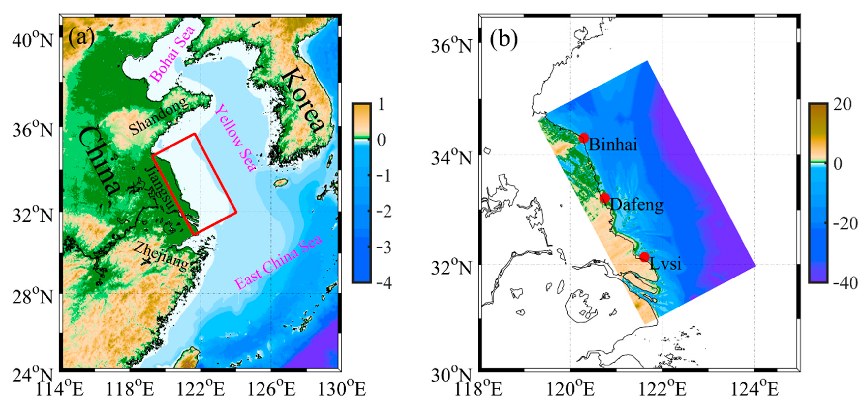
2.1. Model Setup
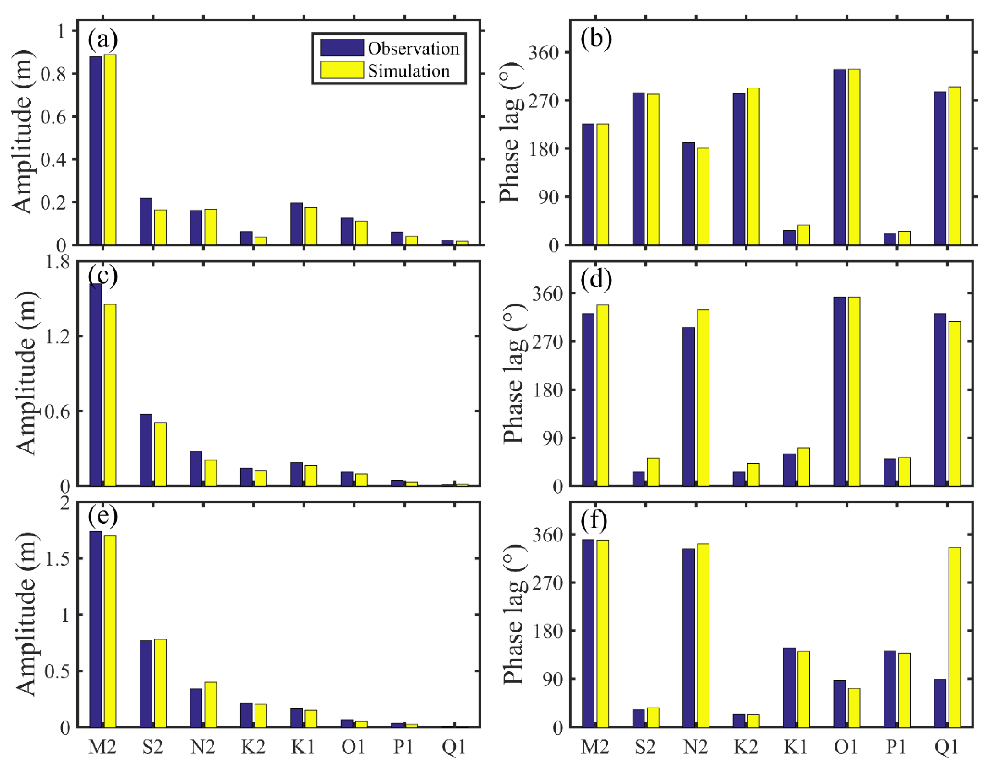
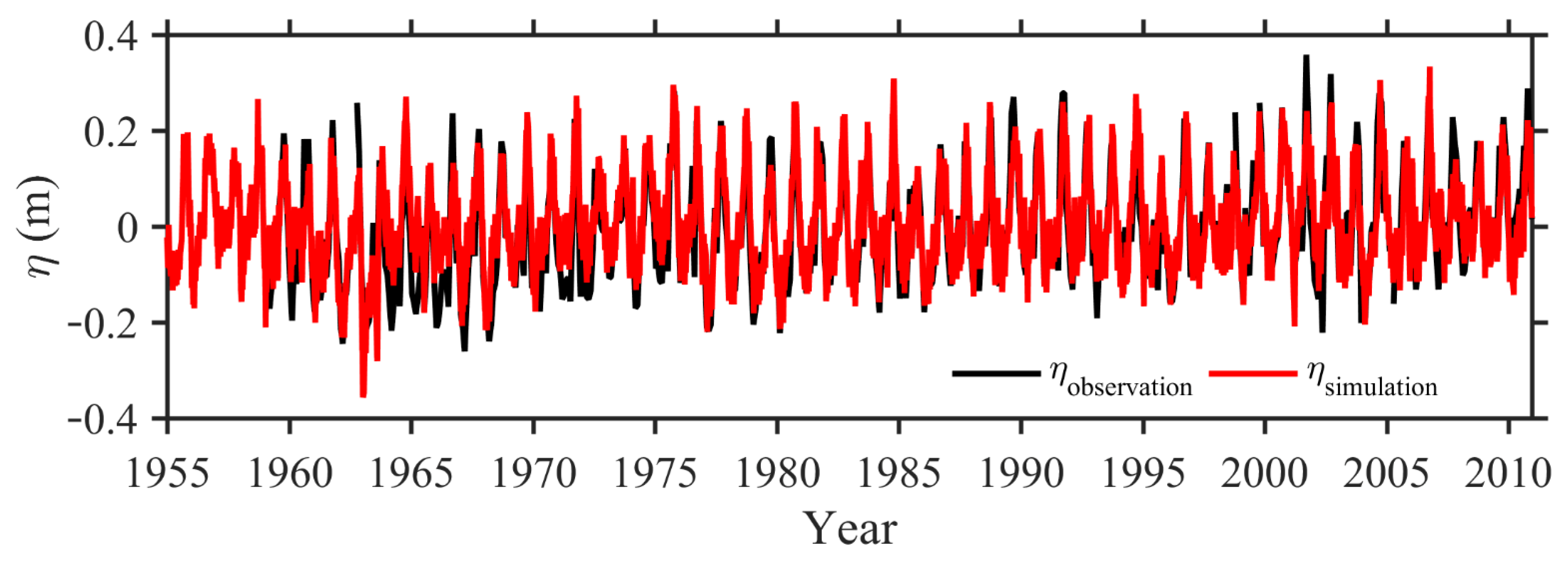
2.2. Model Validation
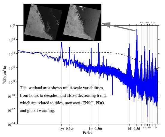
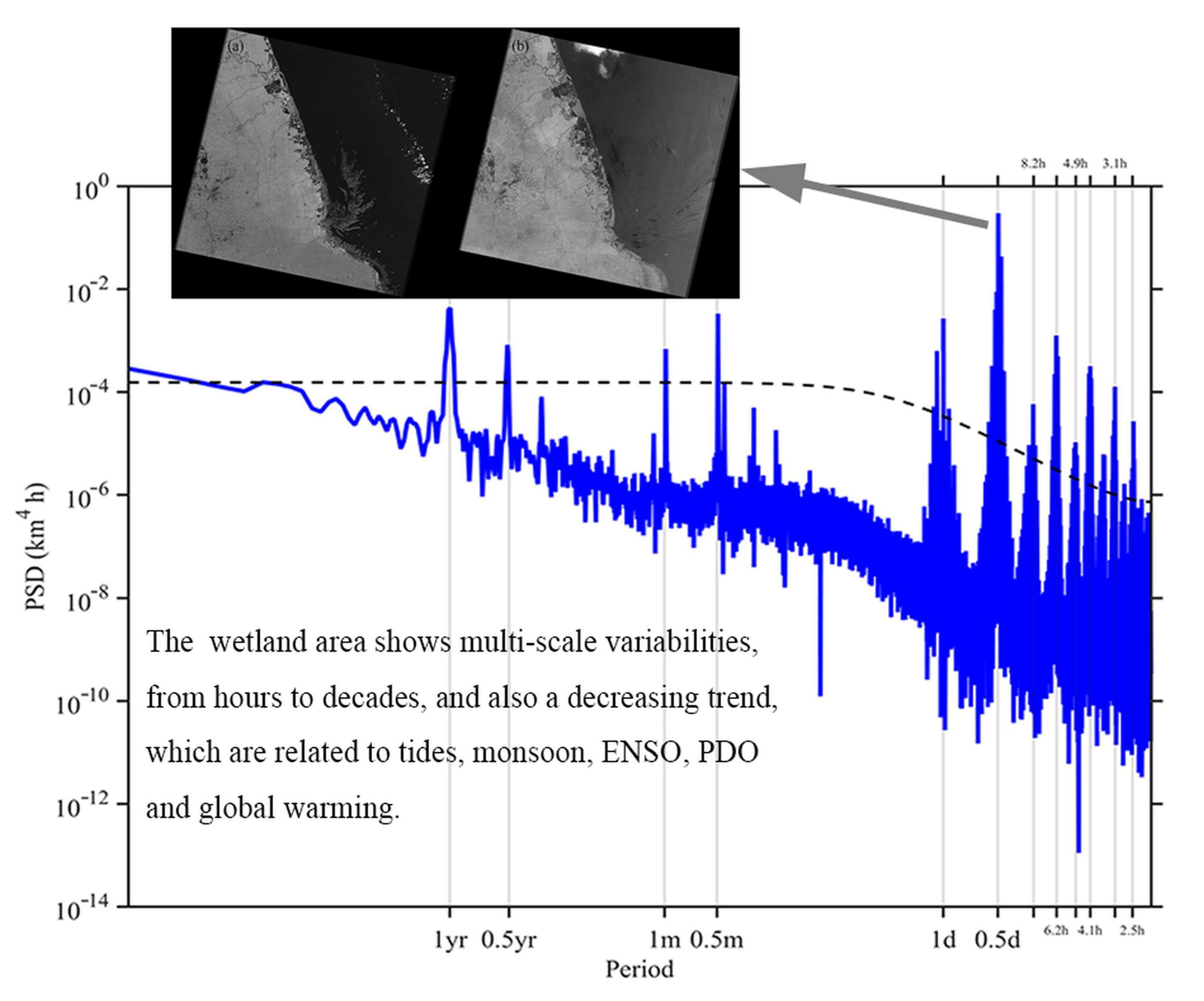
2.3. Definition of Wetland Variability
3. Results
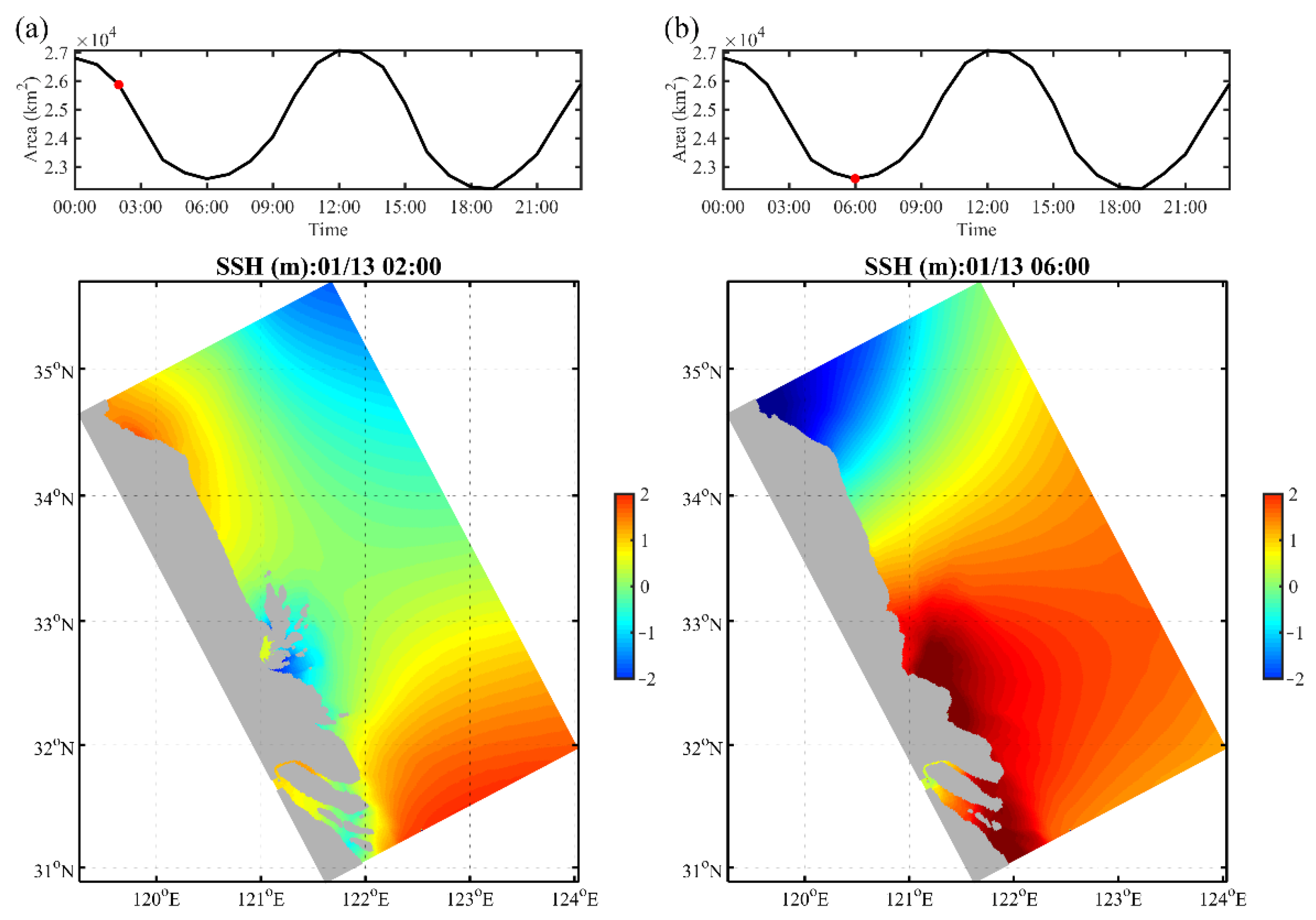
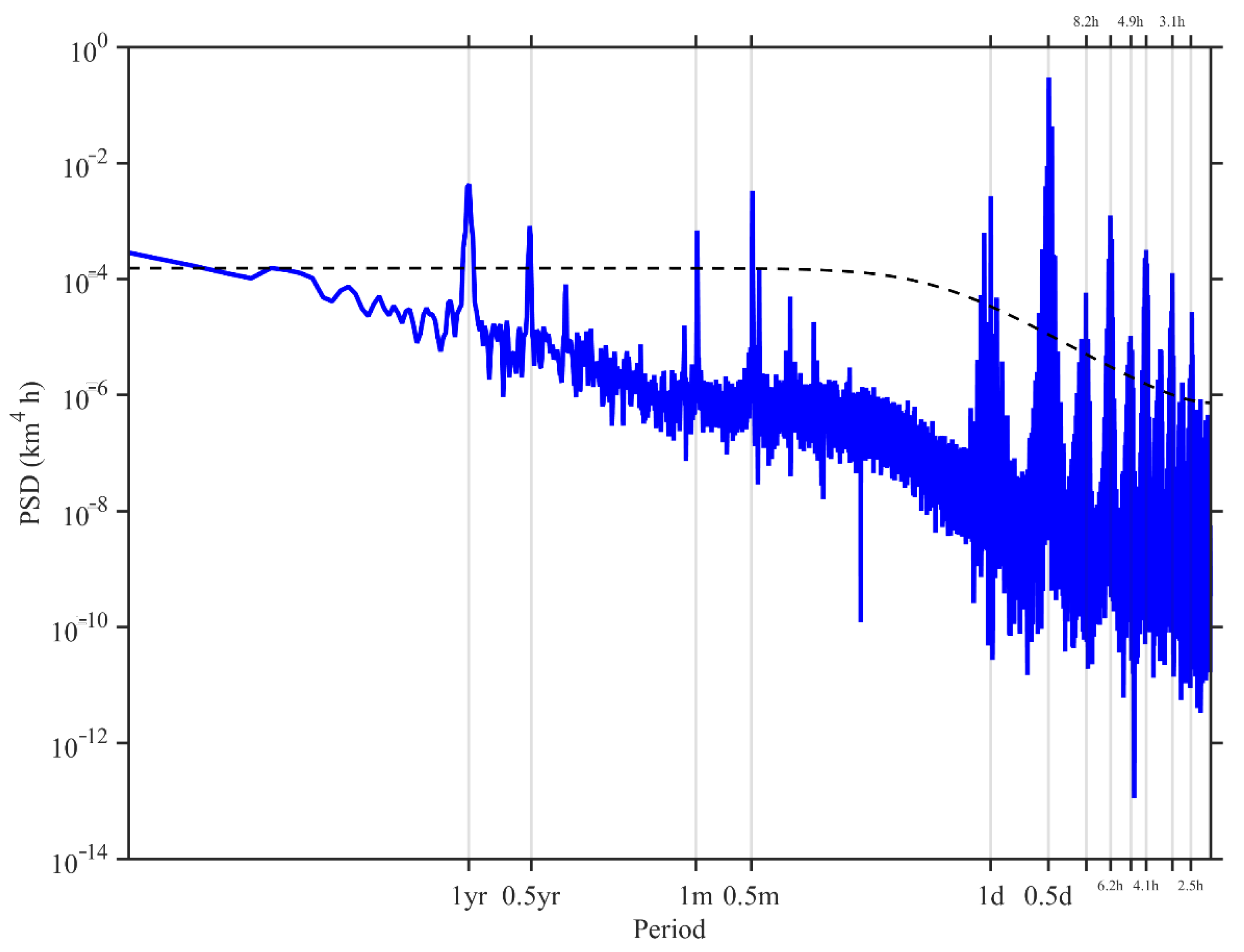
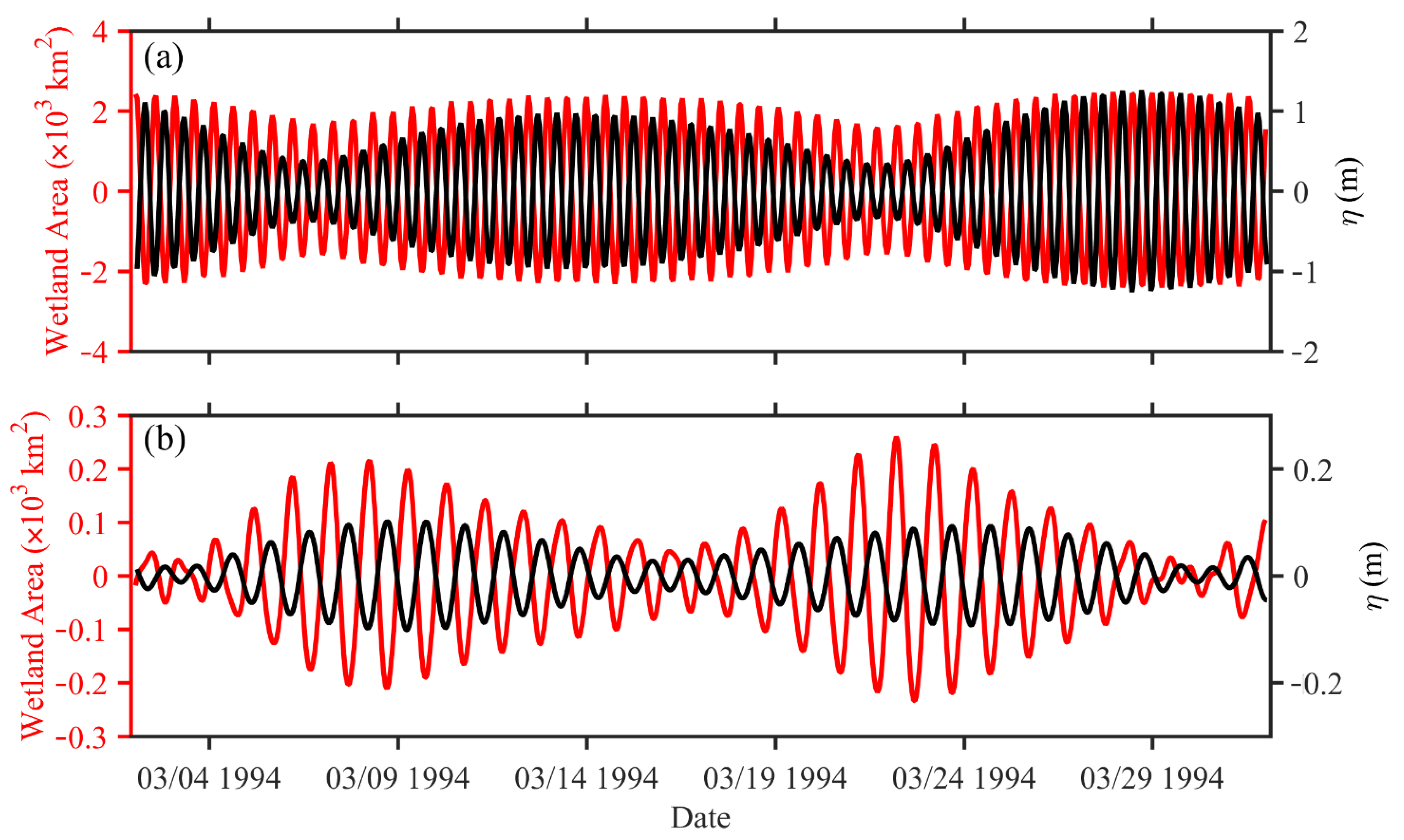
3.1. Intra-Seasonal Variation
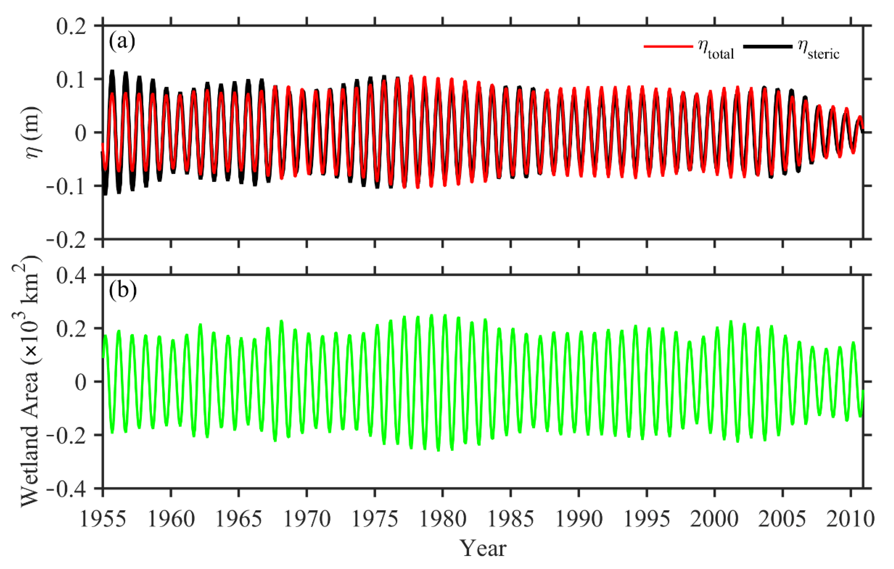
3.2. Seasonal Variation
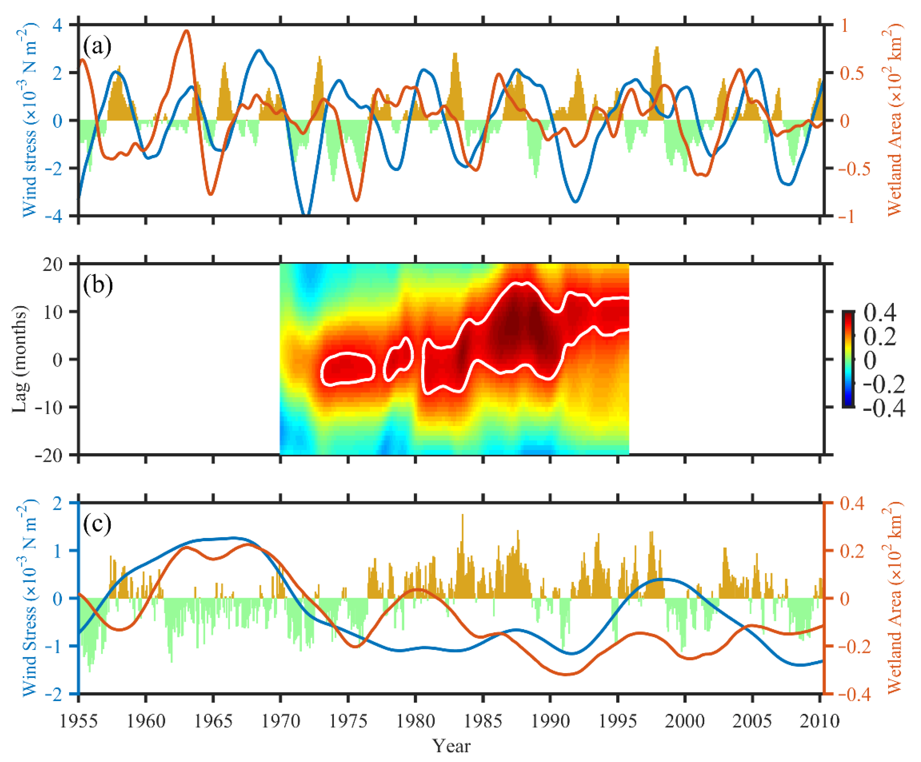
3.3. Interannual and Decadal Variations
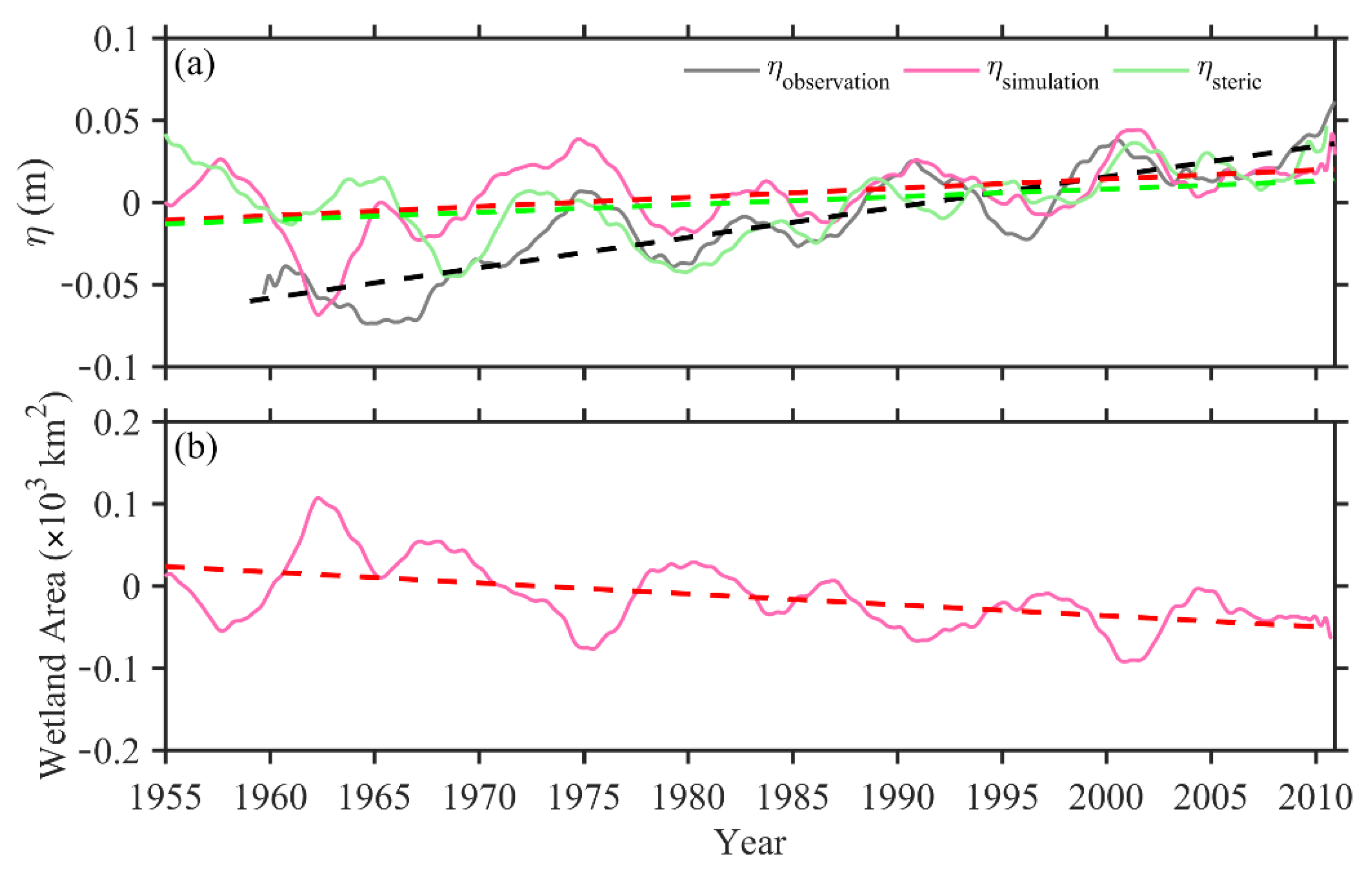
3.4. Long-Term Variation Trend
4. Discussion
4.1. Wind Contribution to Diurnal and Seasonal Wetland Area Variabilities
4.2. The Contribution of Sea Level Rise
4.3. Limitations of the Model
5. Conclusions
Author Contributions
Funding
Institutional Review Board Statement
Informed Consent Statement
Data Availability Statement
Acknowledgments
Conflicts of Interest
References
- Denny, P. Biodiversity and wetlands. Wetl. Ecol. Manag. 1994, 3, 55–611. [Google Scholar] [CrossRef]
- Tiner, R.W. Wetlands of the United States: Current Status and Recent Trends; United States Fish and Wildlife Service: Washington, DC, USA, 1984; 59p.
- UNEP (United Nations Environment Programme). Marine and Coastal Ecosystems and Human Wellbeing: A Synthesis Report Based on the Findings of the Millennium Ecosystem Assessment; UNEP: Nairobi, Kenya, 2006; 76p. [Google Scholar]
- McGranahan, G.; Balk, D.; Anderson, B. The rising tide: Assessing the risks of climate change and human settlements in low elevation coastal zones. Environ. Urban. 2007, 19, 17–37. [Google Scholar] [CrossRef]
- Lubchenco, J.; Menge, B.A. Community Development and Persistence in a Low Rocky Intertidal Zone. Ecol. Monogr. 1978, 48, 67–94. [Google Scholar] [CrossRef] [Green Version]
- Black, K.S.; Paterson, D.; Cramp, A. (Eds.) Sedimentary Processes in the Intertidal Zone; Geological Society: London, UK, 1998; 139p. [Google Scholar]
- Commito, J.A.; Como, S.; Grupe, B.; Dow, W.E. Species diversity in the soft-bottom intertidal zone: Biogenic structure, sediment, and macrofauna across mussel bed spatial scales. J. Exp. Mar. Biol. Ecol. 2008, 366, 70–81. [Google Scholar] [CrossRef]
- Costanza, R.; Pérez-Maqueo, O.; Martinez, M.L.; Sutton, P.; Anderson, S.J.; Mulder, K. The Value of Coastal Wetlands for Hurricane Protection. AMBIO 2008, 37, 241–248. [Google Scholar] [CrossRef]
- Chen, S.; Geyer, W.R.; Sherwood, C.R.; Ralston, D.K. Sediment transport and deposition on a river-dominated tidal flat: An idealized model study. J. Geophys. Res. Earth Surf. 2010, 115, C10040. [Google Scholar] [CrossRef] [Green Version]
- Davidson, N.C. How much wetland has the world lost? Long-term and recent trends in global wetland area. Mar. Freshw. Res. 2014, 65, 934–941. [Google Scholar] [CrossRef]
- Michener, W.K.; Blood, E.R.; Bildstein, K.L.; Brinson, M.M.; Gardner, L.R. Climate Change, Hurricanes and Tropical Storms, and Rising Sea Level in Coastal Wetlands. Ecol. Appl. 1997, 7, 770–801. [Google Scholar] [CrossRef]
- Morris, J.T.; Sundareshwar, P.V.; Nietch, C.T.; Kjerfve, B.; Cahoon, D.R. Responses of coastal wetlands to rising sea level. Ecology 2002, 83, 2869–2877. [Google Scholar] [CrossRef]
- Cazenave, A.; Le Cozannet, G. Sea level rise and its coastal impacts. Earths Futur. 2014, 2, 15–34. [Google Scholar] [CrossRef]
- Nicholls, R.J.; Cazenave, A. Sea-Level Rise and Its Impact on Coastal Zones. Science 2010, 328, 1517–1520. [Google Scholar] [CrossRef] [PubMed]
- List, J.H.; Sallenger, A.H.; Hansen, M.E.; Jaffe, B.E. Accelerated relative sea-level rise and rapid coastal erosion: Testing a causal relationship for the Louisiana barrier islands. Mar. Geol. 1997, 140, 347–365. [Google Scholar] [CrossRef]
- Ericson, J.P.; Vorosmarty, C.; Dingman, S.L.; Ward, L.G.; Meybeck, M. Effective sea-level rise and deltas: Causes of change and human dimension implications. Glob. Planet. Chang. 2006, 50, 63–82. [Google Scholar] [CrossRef]
- Morton, R.A. Historical Changes in the Mississippi-Alabama Barrier-Island Chain and the Roles of Extreme Storms, Sea Level, and Human Activities. J. Coast. Res. 2008, 246, 1587–1600. [Google Scholar] [CrossRef]
- Uehara, K.; Sojisuporn, P.; Saito, Y.; Jarupongsakul, T. Erosion and accretion processes in a muddy dissipative coast, the Chao Phraya River delta, Thailand. Earth Surf. Process. Landforms 2010, 35, 1701–1711. [Google Scholar] [CrossRef]
- Niu, Z.; Zhang, H.; Wang, X.; Yao, W.; Zhou, D.; Zhao, K.; Zhao, H.; Li, N.; Huang, H.; Li, C.; et al. Mapping wetland changes in China between 1978 and 2008. Chin. Sci. Bull. 2012, 57, 2813–2823. [Google Scholar] [CrossRef] [Green Version]
- Han, G.; Huang, W. Pacific Decadal Oscillation and Sea Level Variability in the Bohai, Yellow, and East China Seas. J. Phys. Oceanogr. 2007, 38, 2772–2783. [Google Scholar] [CrossRef]
- Bao, X.; Gao, G.; Yan, J. Three dimensional simulation of tide and tidal current characteristics in the East China Sea. Oceanol. Acta 2001, 24, 135–149. [Google Scholar] [CrossRef] [Green Version]
- Liu, X.; Liu, Y.; Guo, L.; Rong, Z.; Gu, Y.; Liu, Y. Interannual changes of sea level in the two regions of East China Sea and different responses to ENSO. Glob. Planet. Chang. 2010, 72, 215–226. [Google Scholar] [CrossRef]
- Shchepetkin, A.F.; McWilliams, J.C. The regional oceanic modeling system (ROMS): A split-explicit, free-surface, topography-following-coordinate oceanic model. Ocean Model. 2005, 9, 347–404. [Google Scholar] [CrossRef]
- Warner, J.C.; Defne, Z.; Haas, K.; Arango, H.G. A wetting and drying scheme for ROMS. Comput. Geosci. 2013, 58, 54–61. [Google Scholar] [CrossRef] [Green Version]
- Dai, A.; Qian, T.; Trenberth, K.E.; Milliman, J.D. Changes in Continental Freshwater Discharge from 1948 to 2004. J. Clim. 2009, 22, 2773–2792. [Google Scholar] [CrossRef]
- Geng, X.; Boufadel, M.C.; Jackson, N.L. Evidence of salt accumulation in beach intertidal zone due to evaporation. Sci. Rep. 2016, 6, 31486. [Google Scholar] [CrossRef] [PubMed]
- Zhao, S.; Liu, X.; Cheng, D.; Liu, G.; Liang, B.; Cui, B.; Bai, J. Temporal–spatial variation and partitioning prediction of antibiotics in surface water and sediments from the intertidal zones of the Yellow River Delta, China. Sci. Total Environ. 2016, 569, 1350–1358. [Google Scholar] [CrossRef] [PubMed]
- Fang, G.; Wang, Y.; Wei, Z.; Choi, B.H.; Wang, X.; Wang, J. Empirical cotidal charts of the Bohai, Yellow, and East China Seas from 10 years of TOPEX/Poseidon altimetry. J. Geophys. Res. Earth Surf. 2004, 109, 227–251. [Google Scholar] [CrossRef]
- Egbert, G.D.; Erofeeva, S.Y.; Ray, R.D. Assimilation of altimetry data for nonlinear shallow-water tides: Quarter-diurnal tides of the Northwest European Shelf. Cont. Shelf Res. 2010, 30, 668–679. [Google Scholar] [CrossRef]
- Cao, A.-Z.; Wang, D.-S.; Lv, X.-Q. Harmonic Analysis in the Simulation of Multiple Constituents: Determination of the Optimum Length of Time Series. J. Atmos. Ocean. Technol. 2015, 32, 1112–1118. [Google Scholar] [CrossRef]
- Feng, X.; Tsimplis, M.N.; Marcos, M.; Calafat, F.M.; Zheng, J.; Jordà, G.; Cipollini, P. Spatial and temporal variations of the seasonal sea level cycle in the northwest Pacific. J. Geophys. Res. Ocean. 2015, 120, 7091–7112. [Google Scholar] [CrossRef] [Green Version]
- Bingham, R.J.; Hughes, C.W. Local diagnostics to estimate density-induced sea level variations over topography and along coastlines. J. Geophys. Res. 2012, 117, C01013. [Google Scholar] [CrossRef] [Green Version]
- Naimie, C.E.; Blain, C.A.; Lynch, D.R. Seasonal mean circulation in the Yellow Sea—A model-generated climatology. Cont. Shelf Res. 2001, 21, 667–695. [Google Scholar] [CrossRef]
- Wang, B.; Wu, R.; Fu, X. Pacific–East Asian teleconnection: How does ENSO affect East Asian climate? J. Clim. 2000, 13, 1517–1536. [Google Scholar] [CrossRef]
- Wang, B.; Zhang, Q. Pacific-East Asian teleconnection. Part II: How the Philippine sea anomalous anticyclone is established during El Niño development. J. Clim. 2002, 15, 3252–3265. [Google Scholar] [CrossRef] [Green Version]
- Yu, L. Potential correlation between the decadal East Asian summer monsoon variability and the pacific decadal oscillation. Atmos. Ocean. Sci. Lett. 2013, 6, 394–397. [Google Scholar] [CrossRef]
- Chen, C.L.; Zuo, J.C.; Chen, M.X.; Gao, Z.G.; Shum, C.K. Sea level change under IPCC-A2 scenario in Bohai, Yellow, and East China Seas. Water Sci. Eng. 2014, 7, 446–456. [Google Scholar] [CrossRef]
- Ye, A.; Li, F. Physical Oceanography; Ocean University Press: Qingdao, China, 1992; 684p. (In Chinese) [Google Scholar]
- Chu, P.; Yuchun, C.; Kuninaka, A. Seasonal variability of the Yellow Sea/East China Sea surface fluxes and thermohaline structure. Adv. Atmos. Sci. 2005, 22, 1–20. [Google Scholar] [CrossRef] [Green Version]


| Tides | M2 (12.4 h) | K1 (23.9 h) | O1 (25.8 h) | S2 (12.0 h) | N2 (12.7 h) | P1 (24.1 h) | K1 (12.0 h) | Q1 (26.9 h) |
|---|---|---|---|---|---|---|---|---|
| M2 (12.4 h) | 6.2 h, NAN | \ | \ | \ | \ | \ | \ | \ |
| K1 (23.9 h) | 8.2 h, 1.1 d | 12.0 h, NAN | \ | \ | \ | \ | \ | \ |
| O1 (25.8 h) | 8.4 h, 1.0 d | 12.4 h, 13.7 d | 12.9 h, NAN | \ | \ | \ | \ | \ |
| S2 (12.0 h) | 6.1 h, 14.8 d | 8.0 h, 1.0 d | 8.2 h, 0.9 d | 6.0 h, NAN | \ | \ | \ | \ |
| N2 (12.7 h) | 6.3 h, 27.6 d | 8.3 h, 1.1 d | 8.5 h, 0.4 d | 6.2 h, 9.6 d | 6.3 h, NAN | \ | \ | \ |
| P1 (24.1 h) | 6.2 h, 1.1 d | 12.0 h, 182.7 d | 12.5 h, 14.8 d | 8.0 h, 1.0 d | 8.3 h, 1.1 d | 12.0 h, NAN | \ | \ |
| K1 (12.0 h) | 6.1 h, 13.7 d | 8.0 h, 1.0 d | 6.1 h, 0.5 d | 6.0 h, 182.4 d | 6.2 h, 9.1 h | 8.0 h, 1.0 d | 6.0 h, NAN | \ |
| Q1 (26.9 h) | 8.5 h, 1.0 d | 12.7 h, 9.1 d | 8.5 h, 1.2 d | 8.3 h, 0.9 d | 8.6 h, 1.0 h | 12.7 h, 9.6 d | 8.3 h, 0.9 d | 13.4 h, NAN |
Publisher’s Note: MDPI stays neutral with regard to jurisdictional claims in published maps and institutional affiliations. |
© 2022 by the authors. Licensee MDPI, Basel, Switzerland. This article is an open access article distributed under the terms and conditions of the Creative Commons Attribution (CC BY) license (https://creativecommons.org/licenses/by/4.0/).
Share and Cite
Dong, J.; Dong, C.; Yu, K. Impacts of Climate Change on a Coastal Wetland from Model Simulation Combining Satellite and Gauge Observations: A Case Study of Jiangsu, China. Remote Sens. 2022, 14, 2473. https://0-doi-org.brum.beds.ac.uk/10.3390/rs14102473
Dong J, Dong C, Yu K. Impacts of Climate Change on a Coastal Wetland from Model Simulation Combining Satellite and Gauge Observations: A Case Study of Jiangsu, China. Remote Sensing. 2022; 14(10):2473. https://0-doi-org.brum.beds.ac.uk/10.3390/rs14102473
Chicago/Turabian StyleDong, Jihai, Changming Dong, and Kai Yu. 2022. "Impacts of Climate Change on a Coastal Wetland from Model Simulation Combining Satellite and Gauge Observations: A Case Study of Jiangsu, China" Remote Sensing 14, no. 10: 2473. https://0-doi-org.brum.beds.ac.uk/10.3390/rs14102473