Article

Development and Evaluation of a Real-Time Hourly One-Kilometre Gridded Multisource Fusion Air Temperature Dataset in China Based on Remote Sensing DEM

1
National Meteorological Information Center, China Meteorological Administration, Beijing 100081, China
2
Henan Meteorological Observation Data Center, Zhengzhou 450000, China
3
Meteorological Information Center of Inner Mongolia Autonomous Region, Hohhot 010000, China
*
Author to whom correspondence should be addressed.
Remote Sens. 2022, 14(10), 2480; https://0-doi-org.brum.beds.ac.uk/10.3390/rs14102480
Submission received: 8 March 2022 / Revised: 7 May 2022 / Accepted: 19 May 2022 / Published: 22 May 2022
(This article belongs to the Special Issue Environmental Health Diagnosis Based on Remote Sensing)

Abstract

:
High-resolution gridded 2 m air temperature datasets are important input data for global and regional climate change studies, agrohydrologic model simulations and numerical weather predictions, etc. In this study, the digital elevation model (DEM) is used to correct temperature forecasts produced by ECMWF. The multi-grid variation formulation method is then used to fuse the data from corrected temperature forecasts and ground automatic station observations. The fused dataset covers the area over (0–60°N, 70–140°S), where different underlying surfaces exist, such as plains, basins, plateaus, and mountains. The spatial and temporal resolutions are 1 km and 1 h, respectively. The comparison of the fusion data with the verification observations, including 2400 weather stations, indicates that the accuracy of the gridded temperature is superior to European Centre for Medium-Range Weather Forecasts (ECMWF) data. This is because a more significant number of stations and high-resolution terrain data are used to generate the fusion data than are utilized in the ECMWF. The obtained dataset can describe the temperature feature of peaks and valleys more precisely. Due to its continuous temporal coverage and consistent quality, the fusion dataset is one of China’s most widely used temperature datasets. However, data uncertainty will increase for areas with sparse observations and high mountains, and we must be cautious when using data from these areas.

Graphical Abstract

1. Introduction

Climate change is a global problem. Intensified climate changes will lead to more frequent occurrences of disasters and extreme events, imposing significant challenges to social and economic development [1,2]. In climate change studies, temperature is one of the most important elements, which plays a vital role in sustaining food security, fostering economic growth, and protecting the environment [3,4]. A warming temperature is also the fundamental reason behind those critical issues induced by climate change, such as glacier melt and sea surface rise, etc. In the past several decades, automatic weather stations have continuously increased across the globe. As a result, observations can better reflect temperature changes in different world regions, which makes statistical research more spatially representative and conclusions of temperature changes more accurate. However, limited ground observations still cannot meet the needs of numerical weather and climate modeling studies over the vast global area and diverse surface types [5,6].
In recent years, there is a growing demand for high-resolution gridded fused data in meteorological research and operational application, especially in mesoscale modeling studies and operational services for refining forecasts of disastrous weather events [7]. These data are commonly used to provide initial conditions for numerical models, while they are also taken as ‘true values’ to verify simulations at the model grids [8]. In addition, these data are applied to various fields related to climate, including studies of climate change impacts on human health, agriculture, energy, water resources, etc. In these studies, high-resolution datasets that contain fine-scale details effectively improve the accuracy of parameterization schemes used in air quality models, forest fire models, dispersion models, and hydrological models, and thus enhance the accuracy and applicability of these models.
The Real-Time Mesoscale Analysis (RTMA) [9], a real-time high-resolution gridded multisource fusion dataset developed by the National Centers for Environmental Prediction (NCEP), NOAA Earth System Research Laboratory (ESRL), and National Environmental, Satellite, and Data Information Service (NESDIS), was implemented in the NCEP Central Operations in 2006 over a domain that matches the conterminous U.S. National Digital Forecast Database (NDFD) 5 km grid (CONUS RTMA) [10]. In 2008, the RTMA was further applied over domains that match the 6 km Alaska, 2.5 km Hawaii, and 2.5 km Puerto Rico NDFD grids. The two-dimensional variational data assimilation (2DVAR) component used to analyze near-surface observations is described in detail, and the remapping of the NCEP stage II quantitative precipitation amount and NESDIS Geostationary Operational Environmental Satellite (GOES) sounder effective cloud amount to the 5 km grid is briefly discussed [11]. Terrain-following background error covariances are used with the 2DVAR approach, which produces gridded datasets of 2 m temperature, 2 m specific humidity, 2 m dewpoint, 10 m U and V wind components, and surface pressure. The Integrated Nowcasting through Comprehensive Analysis (INCA) developed by the Austrian National Weather Service [12] can construct high-resolution topography, surface index, and vertical coordinate system. In its fusion analysis, real-time surface observations are combined with remote sensing data [13].
On the one hand, the remote sensing data are used to provide spatial structure for the interpolations from real-time observations; on the other hand, the surface observations are used to ensure real-time information in the analysis can be accurately preserved. He et al. [14,15,16] from Qinghua University used the GLDAS NOAH10SUBP 3H temperature data as the background analysis, and error correction for the background analysis was conducted using the ANUSPLIN software package [17,18]. The above work produced a gridded temperature dataset over China with 10 km spatial resolution and 3 h temporal resolution. The U.S. National Oceanic and Atmospheric Administration, National Aeronautics and Space Administration, and other agencies began to develop the North American Land Surface Data Assimilation System in 2004 [19,20,21]. Since then, the NLDAS has been continuously developing in scientific research and operational applications of global and regional land surface data assimilation systems. The NLDAS data has been widely used in the world. At the same time, various land surface data assimilation systems have been developed in other national agencies, including the NASA Famine Early Warning Systems Network (FEWS NET) Land Data Assimilation System (FLDAS) [22], NASA National Climate Assessment-Land Data Assimilation System (NCA-LDAS) [23], and NCAR High-Resolution Land Data Assimilation System (HRLDAS) [24]. Temperatures in these land surface data assimilation systems are often derived from 2 m temperature produced by domestically developed atmosphere data assimilation systems and corrected based on surface observations.
To meet the demand for high-resolution real-time analyses in China and gradually promote the development of surface meteorological analysis products, the National Meteorological Information Center (NMIC) of the China Meteorological Administration (CMA) established a multiphase program in 2012 to develop the China Land Surface Data Assimilation System (CLDAS). In 2017, the Analysis of Real-Time (ART) developed by NMIC of CMA further enhanced the existing analysis capabilities of NMIC to produce 1–5 km resolution analyses of near-surface conditions on grids that match the forecast grids of CMA. The ART has been producing high-resolution analyses of 10 m wind (10 W), 2 m temperature (T2), and relative humidity (RHU) over 0–60°N and 70–140°S on 5 km grids since September 2017, and the analysis products were upgraded to 1 km spatial resolution in 2021.
In the present study, a set of algorithms for fusion has been proposed to produce an hourly, 1 km resolution air temperature dataset of ART in China. High-resolution DEM based on remote sensing data, surface observations collected by automatic weather stations, and numerical predictions are used in data fusion. Characterized by real-time and high spatiotemporal resolutions, accurate gridded T2 data can be used for high-temperature monitoring and cold wave early warning, thus providing disaster prevention and mitigation support. This paper covers the following issues: (1) a brief introduction of data sources and algorithms used for T2 data fusion; (2) evaluation and analysis of product quality; and (3) summary and discussion.

2. Materials and Methods

2.1. Data Sources

2.1.1. Model Background Field

The background fields used in the fusion analysis of air temperature are provided by European Centre for Medium-Range Weather Forecasts (ECMWF) [25,26,27]. ECMWF provides aggregated values for seven parameters: 2 m air temperature, 2 m dewpoint temperature, total precipitation, mean sea level pressure, surface pressure, 10 m u-component of wind, and 10 m v-component of wind. The spatial resolution is 12.5 km × 12.5 km, and the temporal resolution is 3 h.

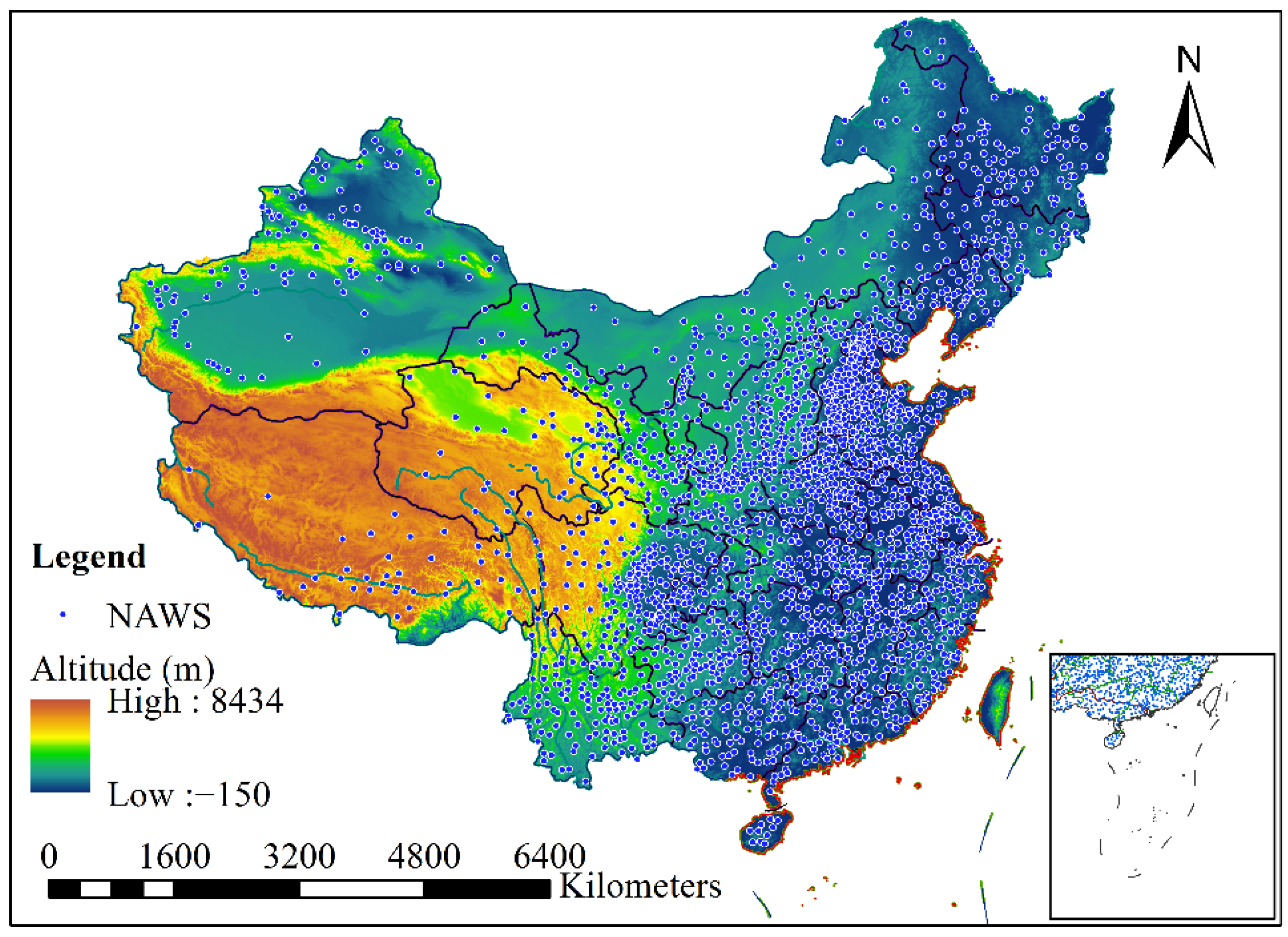
2.1.2. In-Site Observations

Surface data are observations collected at operational automatic weather stations in China. Among these stations, 2400 national-level stations collect 2 m temperature, and 50,000 non-national level stations measure 2 m temperature. All the measurements are conducted at 1 h intervals. Quality control has been conducted before the data are used for fusion, and abnormal data are excluded to avoid their impacts on the fused dataset.

2.1.3. Remote Sensing DEM

In fact, in the development of the multisource fusion algorithm in this paper, a significant data source is the grid-by-grid digital elevation model data based on remote sensing measurement. The high resolution of 1 km DEM data can solve the problem of data fusion in mountain and valley areas with severe fluctuations because the coarse resolution background field can only describe the regional average temperature in these areas but cannot describe the vertical change of temperature in local mountain or valley in detail. By introducing high-resolution terrain data, we can calculate the height difference between the background field terrain and the actual 1 km terrain and calculate the corrected background field through the terrain decline rate. After correction, the background temperature is more consistent with the actual temperature than previously. Therefore, the application of remote sensing DEM data in this paper plays a key role in developing a fusion algorithm.
The NASA Shuttle Radar Topographic Mission (SRTM) has provided digital elevation data (DEMs) for over 80% of the globe. Due to the difference in spatial resolution between the background field and fused data, resampling and elevation correction of the background temperature data need to be conducted before data fusion. The gridded elevation data used in the correction are derived from high-resolution satellite remote sensing data from the Shuttle Radar Topographic Mission (SRTM, http://srtm.csi.cgiar.org/, accessed on 18 July 2019), whose original resolution is 90 m × 90 m. The downloaded data cover the area (0–60°N, 70–140°E). By resampling in the data space, the original digital elevation model (DEM) [28] is remapped to 1 km × 1 km and 12.5 km × 12.5 km grids, respectively, corresponding to the spatial resolution of background analysis and the resolution of the fused data. Differences in elevation at individual grids are then calculated and multiplied by the lapse rate of temperature to obtain the corrected values, which are added to the background temperature to get the corrected background temperature.

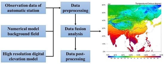
2.2. Data Processing

The test period included 1 January to 31 December 2020, and the background data is forecast data on 12.5 km × 12.5 km grids at 3 h intervals. Hourly data was obtained first by temporal interpolation, and the background analysis on 1 km × 1 km grids at 1 h intervals was then produced by spatial resampling and terrain elevation correction. The observations used in this study were the measurements collected at automatic weather stations of CAM. Every hour, there were about 50,000 valid observations. The observations from national-level automatic weather stations of CMA are reserved for evaluating the test results. These observations in Figure 1 are not used in data fusion to ensure the independence and reliability of the evaluation.

2.3. Fusion Method

The fusion method used in the present study was developed by the NOAA Earth System Research Laboratory [29]. A space-time multiscale analysis (STMAS) can be conducted using this method [29,30]. The variation characteristics of a physical quantity can be taken as the result of the superposition of long waves (larger-scale systems) and short waves (smaller-scale systems) [29]. In the process of fusion, the study area is divided into multi-layer grids of different resolutions, and the number of grids is then used to control the scale of analysis. For a given number of grids in a specified area, only those waves of finite scales can be resolved [29,30]. The more numerous the grid points, the smaller the wave that can be resolved. The analysis started from a coarse-resolution grid, and the result for the coarse-resolution grid is used as the initial condition for analysis in the next layer grid. As the grid is gradually refined, the observation information of different scales is gradually resolved [31].

2.4. Algorithms for Evaluation

The bilinear interpolation method is implemented in this study. The algorithms are written as:
Z ( I 1 , J ) = J J 2 J 1 J 2 Z ( I 1 , J 1 ) + J J 1 J 2 J 1 Z ( I 1 , J 2 )
Z ( I 2 , J ) = J J 2 J 1 J 2 Z ( I 2 , J 1 ) + J J 1 J 2 J 1 Z ( I 2 , J 2 )
A linear interpolation is further conducted along the J-direction:
Z ( I , J ) = I I 2 I 1 I 2 Z ( I 1 , J ) + I I 1 I 2 I 1 Z ( I 2 , J )
where Z(I1,J1), Z (I1,J2), Z (I2,J1), and Z(I2,J2) are values of the variable on the corresponding grids; Z(I1,J) and Z(I2,J) are results at I1 latitude and I2 longitude after the linear interpolation; Z(I,J) is the value at the corresponding station after the interpolation.
The metrics used for data evaluation include mean bias (Bias), root mean square error (RMSE), and correlation coefficient (COR). They are calculated by:
Bias = 1 N i = 1 N ( G i O i )
RMSE = 1 N i = 1 N ( G i O i ) 2
COR = i = 1 N ( G i G i ¯ ) ( O i O i ¯ ) i = 1 N ( G i G i ¯ ) 2 i = 1 N ( O i O i ¯ ) 2
where Oi indicates observations at weather station i (true values), Gi denotes the forcing data interpolated to the given station i, N is the total number of stations used for verification.
The correlation coefficient (COR) indicates the degree of linear correlation between two variables: the larger the value, the better the consistency of the two variables. The root mean square error (RMSE) indicates the dispersion of the sample; the smaller the RMSE is, the closer the data is to the actual value. The mean bias (Bias) refers to the average value of the difference between the simulated and observed values; the smaller the average deviation, the better the simulation result. This paper selects these indicators in evaluation, which can basically judge the data quality.
In terms of processing, this paper uses the NCAR Command Language (NCL) software to process data and draw a spatial distribution map and Origin software to draw a relevant statistical map.

3. Results

This section may be divided into subheadings. It should provide a concise and precise description of the experimental results, their interpretation, as well as the experimental conclusions that can be drawn.

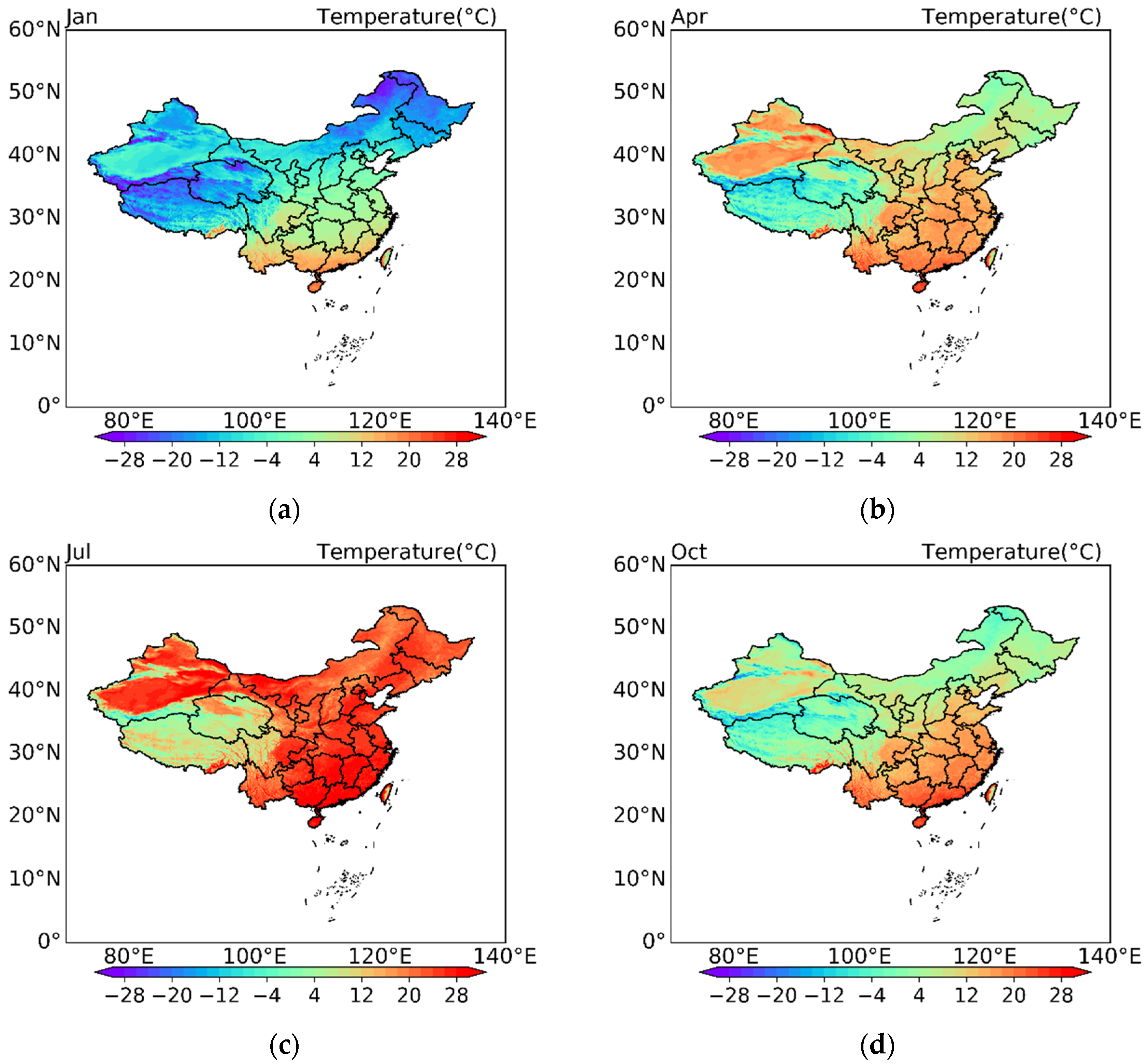
3.1. Spatial Distribution Characteristics in Different Seasons

Monthly mean temperatures are calculated based on the fusion data for the period from January to December 2020 as shown in Figure 2. Detailed analysis of monthly mean temperatures in January, April, July, and October was conducted.
The spatial distribution of the monthly mean temperature in January shows that the isotherm of 0 °C is roughly located along the Qinling–Huaihe Line. Temperature is below 0 °C to the north of this line with freezing winter. The lowest temperature of around −30 °C occurs at Mohe, Heilongjiang Province. To the south of this line, the temperature is above 0 °C and greater than 20 °C on Hainan Island. Therefore, the winter temperature distribution in China is characterized by warm temperatures in the south and cold temperature in the north, and the temperature difference between the north and south is large.
The spatial distribution of temperature in July indicates that in the summer, although the solar zenith angle is relatively low in northern China, the daytime is longer than that in southern China, which partially compensates for the lack of heat caused by the low solar zenith angle. Temperatures are above 20 °C in most areas of China and greater than 28 °C in many areas of southern China. In July, the monthly mean temperature can reach up to 35 °C in Turpan Basin, Xinjiang. Except for areas of high elevation such as the Qinghai–Tibet Plateau, high temperatures are common throughout the country, and there is little difference in temperature between northern and southern China.

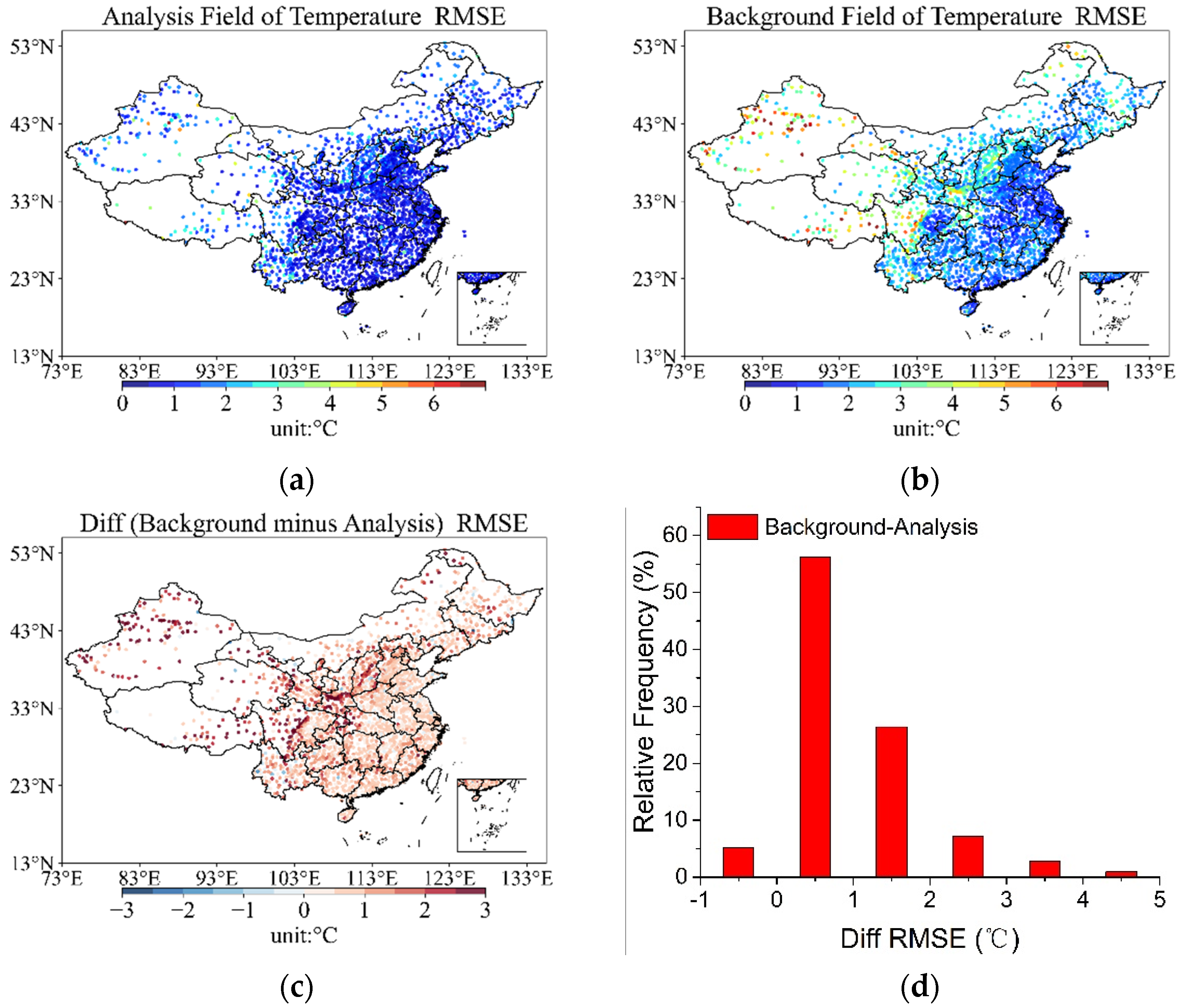
3.2. Evaluation on the Site-Scale

Hourly observations at individual stations for the period 1 January–31 December 2020 are spatially and temporarily matched with the fused data, which are obtained through bi-linear interpolation and fusion of ECMWF analysis product and observations. RMSE, BIAS, and COR are calculated for each station, and statistical analysis is conducted to investigate the improvement of the fused data relative to the background analysis.

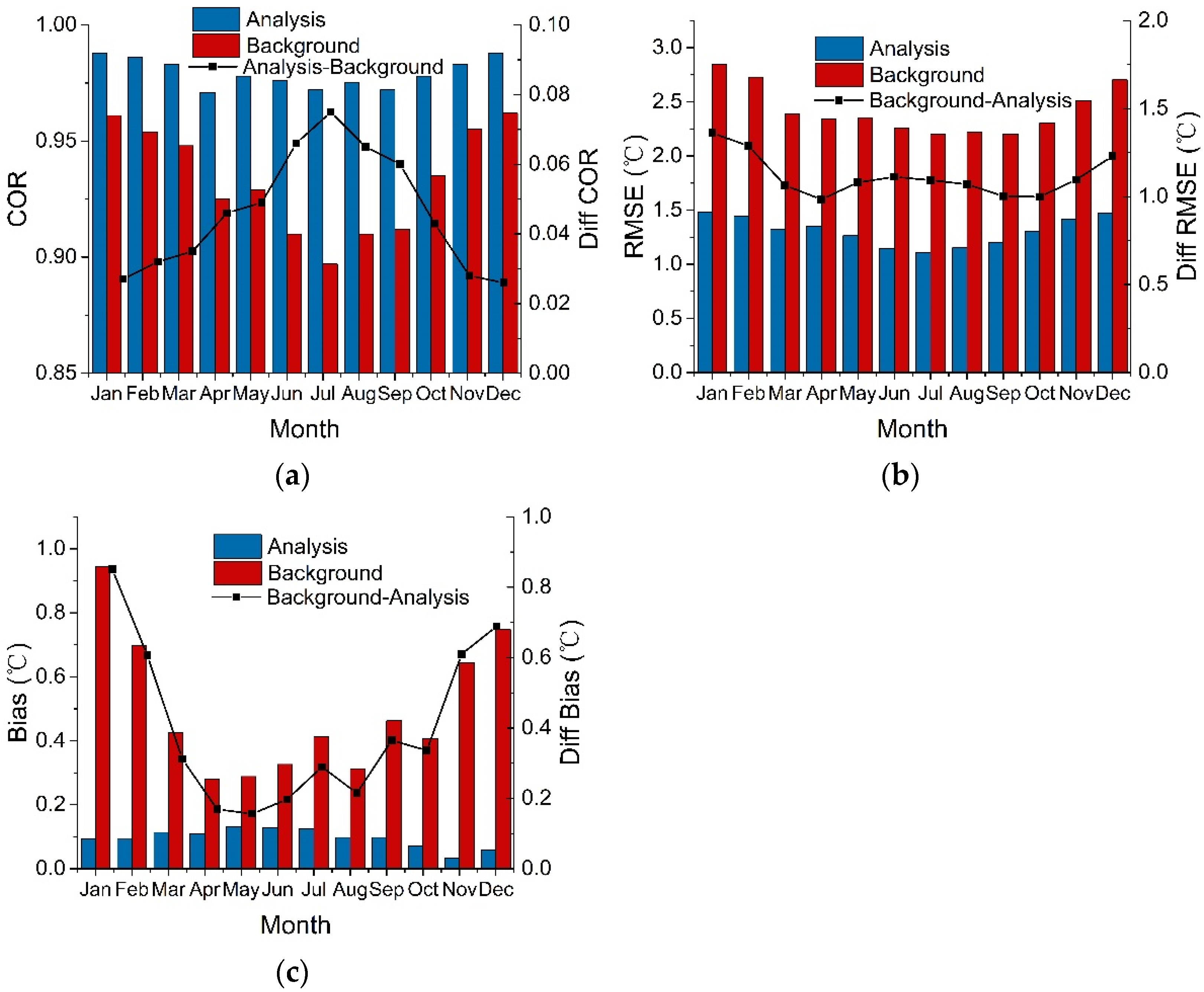
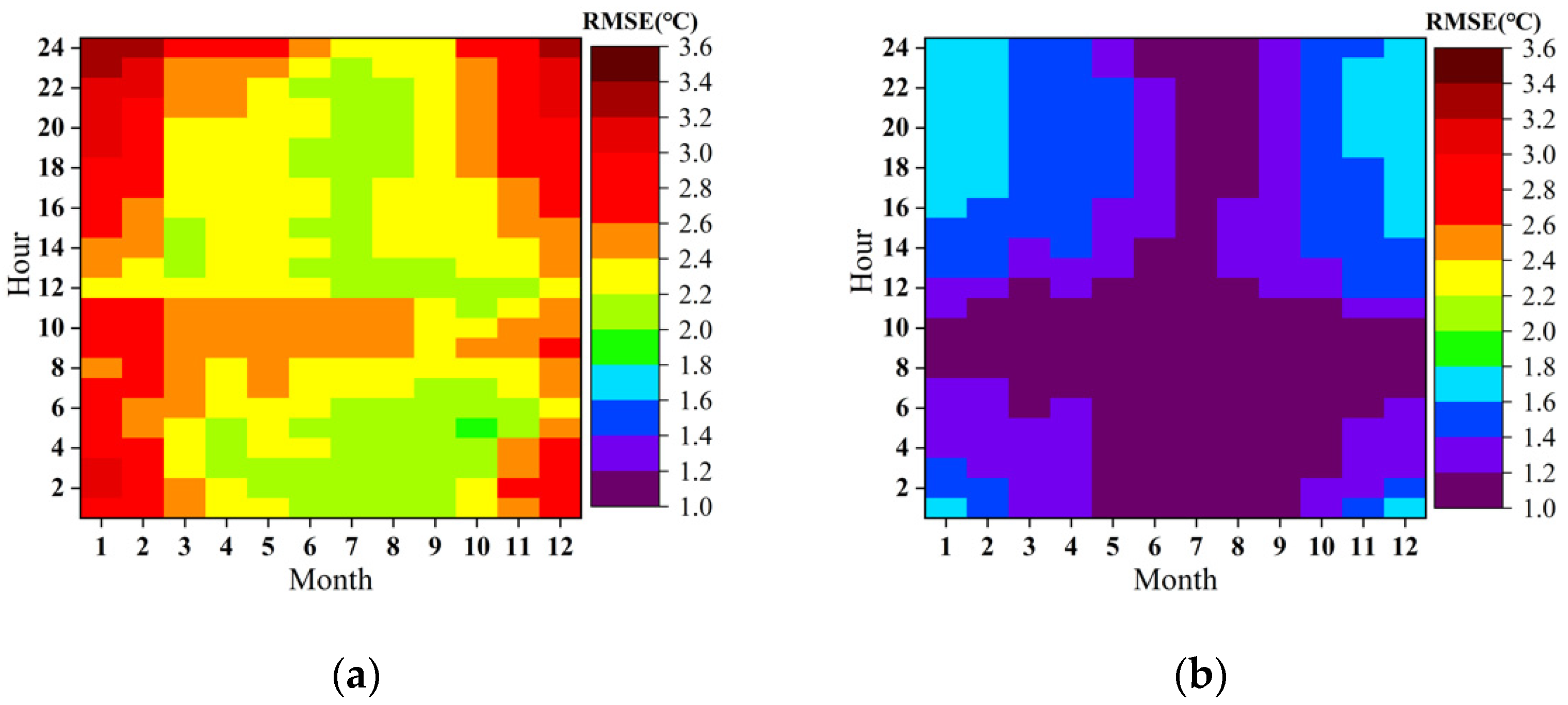
3.2.1. RMSE Analysis
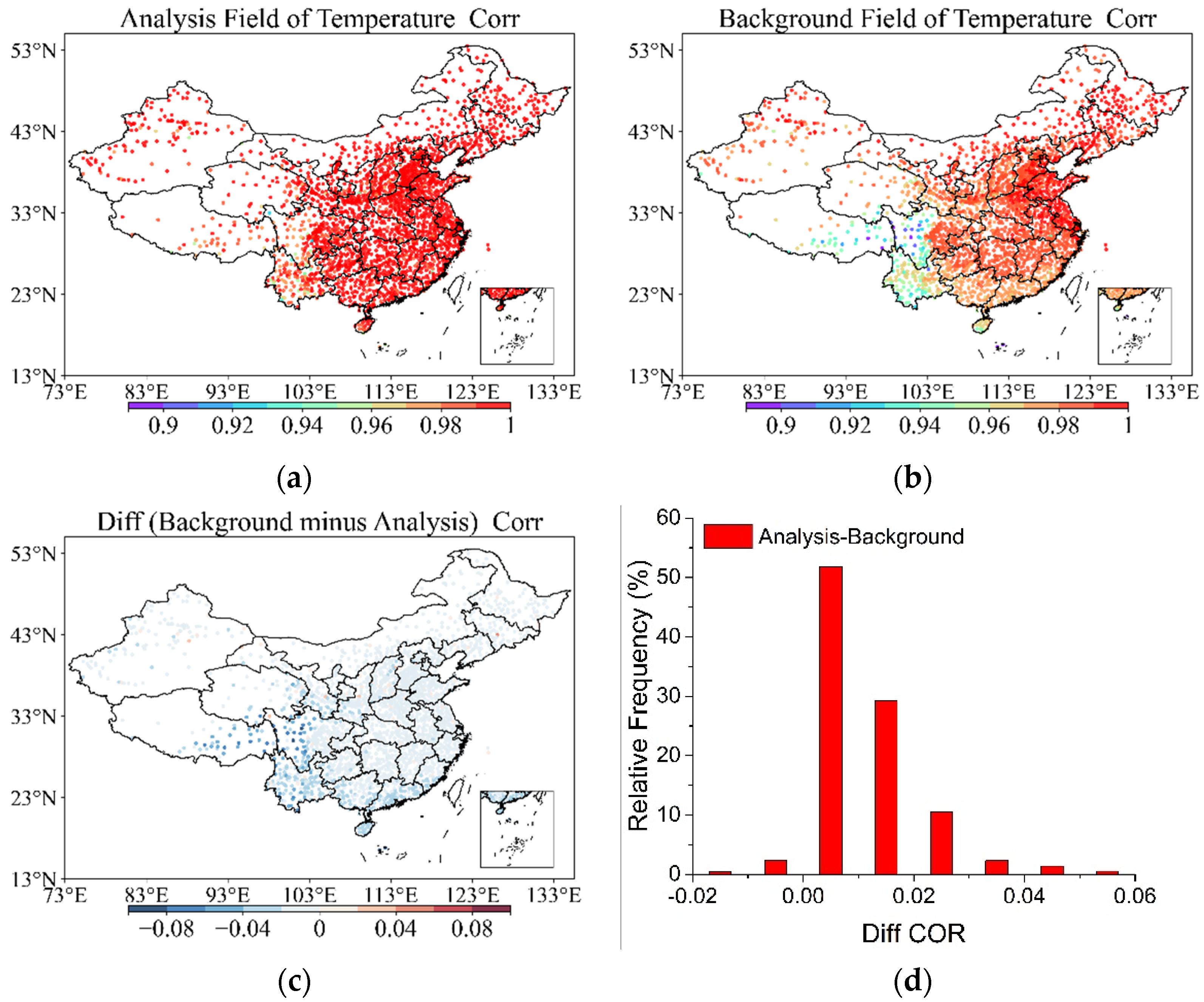
The RMSE of the background analysis in Figure 3 is large in the west and small in the east, demonstrating an obvious spatial distribution characteristic. In most areas of eastern China, the RMSE value is within the range of 1.0 °C~2.5 °C, and a small RMSE is found in the Yangtzi–Huai River Valley, where the RMSE varies between 1.0 °C~1.5 °C. The RMSE is slightly larger in western China, especially in the Qinghai–Tibet Plateau, where the value can be above 3.0 °C. In most areas of China, the RMSE of the fused data is smaller than 1.5 °C and within the range of 2–3 °C over the Qinghai–Tibet Plateau. Overall, the spatial distribution of RMSE indicates that the fused data has been greatly improved compared to the background analysis. Statistical analysis of stations with improved root mean square error shows that the RMSE is improved by 0–1 °C at nearly 55% of the stations and by 1–2 °C at about 25% of the stations. Stations with the RMSE improvement of 0–2 °C account for about 80% of the total stations. Most stations with the RMSE improvement of 2 °C and above are located in the junctions of basins and mountains, where large bias occurs in the coarse-resolution background analysis due to the poor spatial representativeness of observational stations. The fused data demonstrate obvious advantages in these areas with increased spatial resolution, and the data quality is significantly improved.

3.2.2. COR Analysis

The COR of the background analysis in Figure 4 shows an obvious decreasing trend from northeast to southwest. The COR value is above 0.99 in central and eastern China, and it gradually decreased to 0.96–0.98 in the coastal region of southern China. The value is about 0.95 in western Sichuan, Yunnan, and Tibet. At a few individual stations, the COR value is even below 0.92. The COR of the fusion data is generally higher than that of the background analysis, with a value above 0.99 in all the climatic regions of China. Analysis of spatial distribution indicates that the stations with improved COR are concentrated over (93°E–103°E, 23°N–33°N). However, due to the relatively sparse distribution of stations in this region, those stations with a larger than 0.01 improvement of COR only account for less than 30% of the total stations.

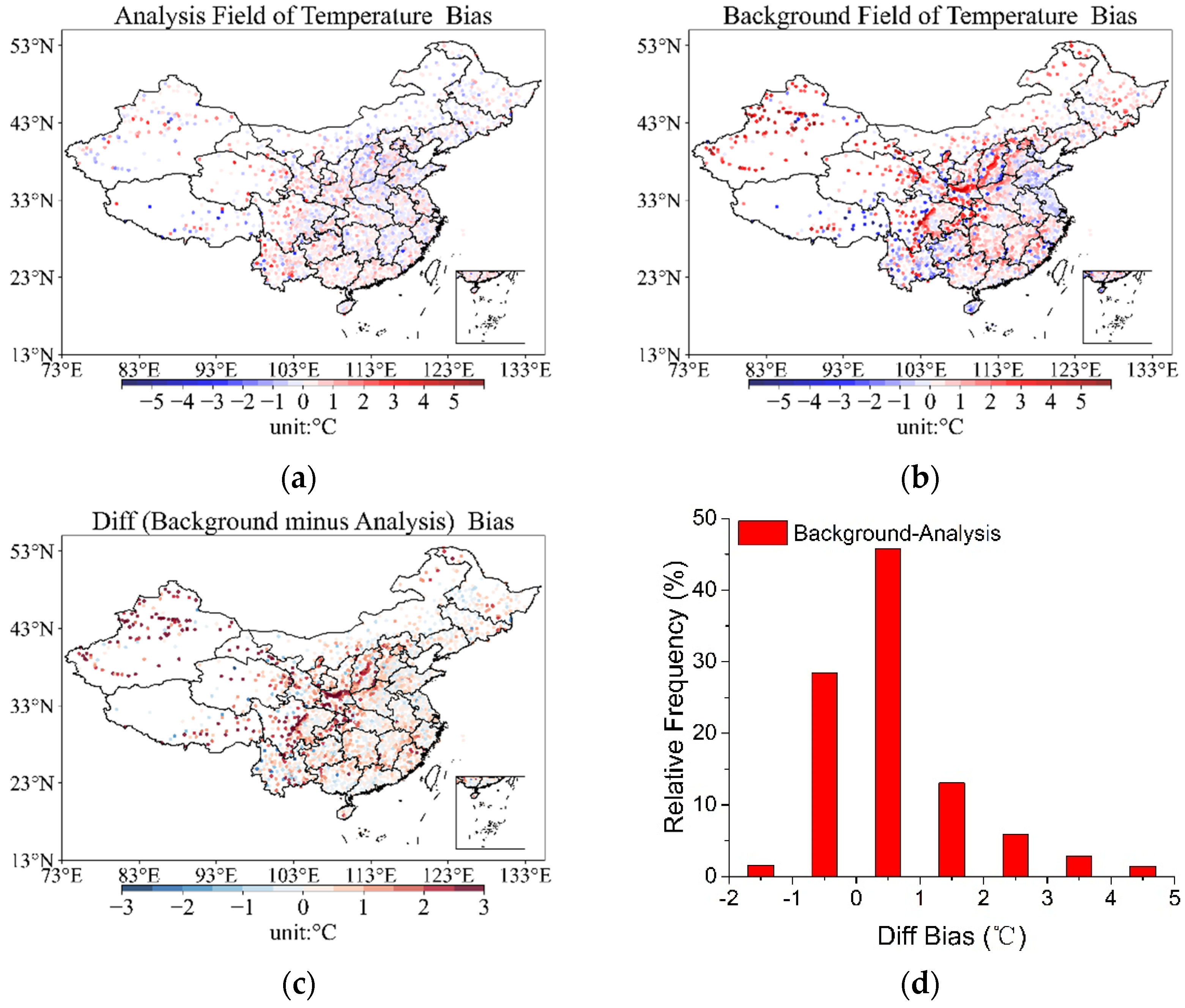
3.2.3. BIAS Analysis

BIAS of the background analysis as depicted in Figure 5 is either positive or negative. In two areas over central-southern China, a large positive bias above 2 °C can be found at certain stations. These stations are located around the Taihang Mountains, the Qinling Mountains, the Hengduan Mountains, etc., where the terrain fluctuates greatly, and the ground station observations are less representative. Bias is significant at these stations due to the low consistency between stations and grids of the analysis data. A slight negative bias is common at stations in coastal areas of eastern China and southwestern China. Spatial BIAS distribution of fused data indicates that the bias is within the range of −1 to 1 in most areas of China. There is no regional-scale systematic bias. The frequency distribution of stations with changed correlation coefficients suggests that the number of stations with the correction value before −1 to 1 is the largest.

3.3. Evaluation for Time Series

To further analyze the improvement in different seasons after fusion analysis, the background and the fused data were evaluated on a monthly basis, and the differences between the two in different months were compared in Figure 6. The number of samples used in each month was about 1,728,000 (n = 1,728,000), and the statistical results passed the significance level test of 0.05 (p < 0.05).
The results of evaluation based on COR, RMSE, and BIAS indicate that the background analysis product is of high quality in the summer, and the BIAS gradually increases in the spring and autumn with decreasing COR. The data quality is the worst in winter among the four seasons. After the improvement by using fusion analysis technology, the evaluation metrics of the fused data distinctly improved in all months. The COR most significantly increased by 0.08 in July, and RMSE shows a consistent improvement in each month, reducing the value by about 1 °C–1.5 °C. The improvement of BIAS is the most obvious. Compared with the background analysis, the BIAS of the fused data is below 0.1 °C in each month, and the improvement was the largest in January and December with the BIAS value decreased by above 0.6 °C.
In addition to the data quality analysis on a monthly basis, monthly mean 24 h error variation in different months is also worthy of attention since this information has important implications for the application of the fused data in Figure 7. Results for the background analysis show that hourly RMSE overall is within 2.0–3.6 °C, and the smallest RMSE occurs at the central point (12 UTC July), from which the RMSE gradually increased (around July to January and July to December, 12 UTC to 00 UTC and 12 UTC to 24 UTC). The hourly RMSE of fused data is significantly better than that of the background analysis each month, with the overall value around 1.2–1.8 °C. Again, the smallest RMSE occurs at the central point (12 UTC July) with the value of about 1.0–1.2 °C, from which the RMSE gradually increases (around July to January and July to December, 12 UTC to 00 UTC and 12 UTC to 24 UTC).

3.4. Evaluation in Different Climatic Regions

Based on comprehensive consideration of the province division and climatic zone division, China is divided into eight regions: North, Northeast, East, Central, South, Northwest, Southwest, and Tibet. The provinces located in each region are listed in Table 1. The geographic locations of the eight regions are denoted by different colors, as shown in Figure 8.
According to the rules for regional division, ground observation stations used for the evaluation are divided into eight regions. In each region, the annual time series of RMSE at individual stations inside the region were calculated and used as samples for statistical analysis. The median, 25% quantile, 75% quantile, upper boundary, lower boundary, and other statistical metrics were then calculated to generate box diagrams for background and fused data. Note that the box contains most of the normal data, and the data outside the upper and lower boundaries of the box are treated as abnormal data.
Figure 9 and Figure 10 display the respective box plots of RMSE for the background analysis and the fused data in different regions. The dispersion and distribution of RMSE at all stations in each region are statistically analyzed, while abnormal data (outliers) are also displayed. The box contains the data between the upper and lower quartiles, that is, 50% of the entire samples. Therefore, the height of the box, to some extent, reflects how fluctuating the data are. Box plots of RMSE for the background analysis in different regions show that the boxes for regions VI (Northwest China), VII (Southwest China), and VIII (Tibet China) are higher than those for other regions, indicating that RMSE varies significantly in these regions. Furthermore, the mean RMSE in these regions is also larger than in other regions, and more outliers can be found in these regions. Overall, background data quality in these regions is lower than in other regions. Compared with the evaluation results of the background analysis, the box plot of RMSE for the fused data indicates that the RMSE significantly decreases in all the eight regions and shows a more concentrated distribution, suggesting that the quality of the fused data has been greatly improved.

4. Discussion

The present study proposes a method to fuse high-resolution DEM based on remote sensing data with observations collected at ground weather stations and numerical predictions. A set of fusion analysis algorithms has been developed to produce fused 2 m air temperature data on 1 km × 1 km grids in China at 1 h intervals. Independent observations are used to evaluate the fused temperature data and the background analysis for 2020 based on statistical metrics of COR, BIAS, RMSE, etc. The advantages and weaknesses of the fused data are objectively analyzed. The overall evaluation results show that through merging multiple data sources, the quality of fused temperature is significantly better than that of the background field.
Using the INCA system, Chen et al. [7] produced a gridded temperature dataset over Zhejiang of China. Observations collected in Zhejing are fused with ECMWF reanalysis to generate a gridded temperature dataset with a 1 km spatial resolution and 1 h temporal resolution. Although this method can effectively improve the quality of background reanalysis, cross-validation results indicate that the number and locations of observation stations significantly impact the evaluation of the gridded dataset, especially over high-elevation areas and coastal regions with few observation stations. At present, the dataset produced by Chen et al. [7] can only cover Zhejiang, where observations are relatively dense and the terrain is flat. The applicability of this method in China, where the distribution of observation stations is extremely uneven, and the staircase-like terrain is obviously high in the west and low in the east, has not been reported. The spatial scope selected for the present study covers all of China, where different types of climatic regions and different terrain elevations can be found. At the same time, the density of observational data also varies significantly in the study area. The algorithms used in the present study overcame the problems during the data fusion process and produced a gridded temperature dataset covering all of China. Furthermore, the data quality was also effectively improved.
He et al. [14] from Qinghua University developed the CMFD dataset and evaluated the quality of temperature data extracted from this dataset and GLDAS temperature data over China. The results indicated that the RMSE and BIAS of CMFD were smaller than GLDAS, while the COR of CMFD was higher than that of GLDAS. Overall, the quality of CMFD was better than that of GLDAS. Meanwhile, the qualities of CMFD and GLADS were specifically evaluated over Qinghai–Tibet Plateau, and a similar result was found. This dataset has been applied in the monitoring of forest resilience in Southwest China, the distribution of global climate resources, the long-term changes of lake area in the inland basin of the Qinghai–Tibet Plateau and its relationship with climate, the construction of a comprehensive drought index for characteristics of large-scale drought and other studies [32]. However, note that there are some constraints in the development of this dataset, i.e., currently, temperature observations are collected at nearly 50,000 automatic weather stations in China, but only a subset of these observations at about 700 stations are used in the development of the CMFD dataset [14]. There is a large gap between the present study and the study of He et al. regarding the observations used. At the same time, CMFD has not been updated and released in real time, which makes it difficult to apply this dataset for studies of meteorological disasters after 2018.
Ji et al. [8] compared all available air temperature data from GHCN weather stations recorded from 2001 to 2010 with GLDAS fused gridded temperature data over the U.S. They also evaluated this data using the consistency index. Meanwhile, the Daymet 1 km resolution gridded temperature data are taken as ‘true’ temperature and used to evaluate GLDAS temperature grid-by-grid. Temperature change trends in different regions and data reliability at different elevations were analyzed. Results indicate that GLDAS temperature data are generally accurate on a regional and global scale. The accuracy of maximum temperature is higher than that of minimum temperature, the accuracy in South America and Africa is lower than that in other regions, and the accuracy and stability of GLDAS temperature in alpine regions are relatively low [8]. As a global dataset, its horizontal resolution is 25 km, temporal resolution is 3 h, and is appropriate for a global-scale climate change study. However, this dataset did not meet the criteria for a regional scale gridded temperature dataset with high accuracy. The dataset developed in the present study has a spatial resolution of 1 km and temporal resolution of 1 h, which upgrades the study from mesoscale to microscale and can more abundantly and reasonably reflect the details of local temperature changes.
In addition to the above research, the geostatistical method is also a common interpolation method [33]. Geostatistical interpolation methods, such as inverse distance weighting or Kriging interpolation, derive a prediction surface from the measured values of sampling points [34], which is used to estimate the values of spatial continuous phenomena in all other locations in a study area [35]. The prediction made by geostatistical interpolation can be decomposed into a deterministic trend and a random error component of spatial autocorrelation; the deterministic trend component can be expressed as the result of a constant average that does not depend on the position or a function that the average changes with the position [36]. The spatial autocorrelation random error component represents the local change of the surface. However, no matter which geostatistical method, the search radius and the minimum number of observation points are specified in the interpolation process. The sparse stations will significantly impact the interpolation results [37]. The spatial distribution map of 2400 ground automatic weather stations in China are shown in Figure 1 with obvious density differences. In the eastern region, the station density is large, but with the rise of altitude and the increase of topographic relief, the distribution of automatic stations is gradually sparse in the western region [38], especially in the Qinghai–Tibet Plateau [39]. In this case, the geostatistical method is directly used to interpolate the station observations to form a grid temperature data set. The quality of the data set will be significantly affected by the station density [40], showing heterogeneity in eastern and Western China [41]. However, the multisource data fusion method combined with terrain correction proposed in this study can effectively reduce the impact of station density on data quality [42] because in the space-time multiscale analysis method, the limited stations in the western region can also correct the background field as effectively as possible [43].
Although the temperature data with 1 km resolution has many advantages, it also has many limitations, especially in the area where the vertical change of elevation is relatively fast. In these regions, the spatial variation of air temperature is more obvious. Under the pixel resolution of 1 km [44], it may contain multiple subgrids metadata of different scales [45], especially in the Himalayas. However, due to the limitation of spatial resolution, the current data cannot accurately describe this change. They can only average to the phase elements of the 1 km scale [46], which will be a more significant challenge to the reliability of data sets in similar regions [47]. To solve this problem, we can improve the resolution of the grid, but the resolution improvement will bring a huge amount of computer calculation and storage, and the cost is very high [48]. In the future, Delaunay triangulation [49] may be introduced, which has the advantages of good structure [50], simple data structure, low data redundancy, high storage efficiency, and harmony with irregular ground features [51].
The change of surface cover type will also have a significant fluctuation in the temperature of 2 m above the ground, especially in large regional forests, wetlands, urban agglomerations [52], etc. Specifically, the benefits of urban heat islands will increase the temperature to a certain extent [53], while forests and wetlands may reduce the temperature. The current calculation model mainly considers the temperature distribution in the natural state [54] but does not consider the influence of the underlying surface on the temperature. In the next step, more detailed research will analyze the influence of a variety of human factors and land cover types on the temperature [55].
In future research, to address the unsolved dataset defects, we will introduce satellite inversion data such as terrain, slope, and vegetation index with higher resolution and further improve the data quality by using in-depth learning technologies such as artificial intelligence.

5. Conclusions

The main purpose of this study is to introduce a grid merged 2 m temperature data set integrating multiple data sources and comprehensively analyze the accuracy and applicability of the data set. Based on the use of the space-time multiscale analysis method, the real-time collection of observation data of various ground automatic weather stations in China is quickly integrated with the high-resolution numerical prediction data corrected by terrain to generate the grid temperature data covering the whole of China with 1 km and 1 h spatial-temporal resolutions.
The main evaluation findings on different scales and in different climatic regions indicate that this method can effectively improve the quality of the background analysis. The overall evaluation results over China show that the fused dataset of 2 m temperature can meticulously reproduce the details of the weather process. The correlation coefficient between the ground observations and the fused data reached 0.99, the root mean square error was 1.33 °C, and the average bias was 0.1 °C. The dataset produced by this study can meet the imperative need for gridded real-time meteorological data in the fields of weather and climate, agriculture, ecology, and hydrology. However, we must remember that the data must be used carefully in areas with sparse sites and complex terrain.

Author Contributions

Conceptualization, C.S. and J.G.; methodology, S.H.; software, S.S.; validation, B.X., Y.Z. and Y.X.; formal analysis, S.H.; investigation, S.S.; resources, B.X.; data curation, C.S.; writing—original draft preparation, S.H.; writing—review and editing, C.S.; visualization, S.S. and Z.L.; supervision, J.G.; project administration, J.G.; funding acquisition, C.S. All authors have read and agreed to the published version of the manuscript.

Funding

This research was funded by the National Key Research and Development Program of China (No. 2018YFC1506601), Key Techniques and Data Sets of Land Surface Reanalysis in the Qinghai–Xizang Plateau (No. NMICJY202106).

Acknowledgments

We are very grateful for the helpful input and suggestions from the anonymous reviewers.

Conflicts of Interest

The authors declare no conflict of interest.

References

  1. Zhou, X.; Huang, G.; Li, Y.; Lin, Q.; Yan, D.; He, X. Dynamical Downscaling of Temperature Variations over the Canadian Prairie Provinces under Climate Change. Remote Sens. 2021, 13, 4350. [Google Scholar] [CrossRef]
  2. Lu, C.; Huang, G.; Wang, G.; Zhang, J.; Wang, X.; Song, T. Long-Term Projection of Water Cycle Changes over China Using RegCM. Remote Sens. 2021, 13, 3832. [Google Scholar] [CrossRef]
  3. Han, S.; Liu, B.; Shi, C.; Liu, Y.; Qiu, M.; Sun, S. Evaluation of CLDAS and GLDAS Datasets for Near-Surface Air Temperature over Major Land Areas of China. Sustainability 2020, 12, 4311. [Google Scholar] [CrossRef]
  4. Han, S.; Shi, C.; Xu, B.; Sun, S.; Zhang, T.; Jiang, L.; Liang, X. Development and evaluation of hourly and kilometer resolution retrospective and real-time surface meteorological blended forcing dataset (SMBFD) in China. J. Meteor. Res. 2019, 33, 1168–1181. [Google Scholar] [CrossRef]
  5. Huang, X.; Han, S.; Shi, C. Multiscale Assessments of Three Reanalysis Temperature Data Systems over China. Agriculture 2021, 11, 1292. [Google Scholar] [CrossRef]
  6. Jiang, Y.; Han, S.; Shi, C.; Gao, T.; Zhen, H.; Liu, X. Evaluation of HRCLDAS and ERA5 Datasets for Near-Surface Wind over Hainan Island and South China Sea. Atmosphere 2021, 12, 766. [Google Scholar] [CrossRef]
  7. Chen, F.; Yang, X.; Ji, C.; Li, Y.; Deng, F.; Dong, M. Establishment and assessment of hourly high-resolution gridded air temperature data sets in Zhejiang, China. Meteorol. Appl. 2019, 26, 396–408. [Google Scholar] [CrossRef] [Green Version]
  8. Ji, L.; Senay, G.B.; Verdin, J.P. Evaluation of the Global Land Data Assimilation System (GLDAS) Air Temperature Data Products. J. Hydrometeorol. 2015, 16, 2463–3480. [Google Scholar] [CrossRef]
  9. De Pondeca, M.S.F.V.; Manikin, G.S.; DiMego, G.; Benjamin, S.G.; Parrish, D.F.; Purser, R.J.; Wu, W.-S.; Horel, J.D.; Myrick, D.T.; Lin, Y.; et al. The Real-Time Mesoscale Analysis at NOAA’s National Centers for Environmental Prediction: Current Status and Development. Weather Forecast. 2011, 26, 593–612. [Google Scholar] [CrossRef]
  10. Ancell, B.C.; Mass, C.F.; Cook, K.; Colman, B. Comparison of Surface Wind and Temperature Analyses from an Ensemble Kalman Filter and the NWS Real-Time Mesoscale Analysis System. Weather Forecast. 2014, 29, 1058–1075. [Google Scholar] [CrossRef]
  11. Zhang, M.; De Leon, C.; Migliaccio, K. Evaluation and comparison of interpolated gauge rainfall data and gridded rainfall data in Florida, USA. Hydrol. Sci. J. 2018, 63, 561–582. [Google Scholar] [CrossRef]
  12. Haiden, T.; Kann, A.; Wittmann, C.; Pistotnik, G.; Bica, B.; Gruber, C. The Integrated Nowcasting through Comprehensive Analysis (INCA) System and Its Validation over the Eastern Alpine Region. Weather Forecast. 2011, 26, 166–183. [Google Scholar] [CrossRef]
  13. Kann, A.; Haiden, T.; Von Der Emde, K.; Gruber, C.; Kabas, T.; Leuprecht, A.; Kirchengast, G. Verification of Operational Analyses Using an Extremely High-Density Surface Station Network. Weather Forecast. 2011, 26, 572–578. [Google Scholar] [CrossRef]
  14. He, J.; Yang, K.; Tang, W.; Lu, H.; Qin, J.; Chen, Y.; Li, X. The first high-resolution meteorological forcing dataset for land process studies over China. Sci. Data 2020, 7, 25. [Google Scholar] [CrossRef] [Green Version]
  15. Sheffield, J.; Goteti, G.; Wood, E. Development of a 50-Year High-Resolution Global Dataset of Meteorological Forcings for Land Surface Modeling. J. Clim. 2006, 19, 3088–3111. [Google Scholar] [CrossRef] [Green Version]
  16. Sheffield, J.; Wood, E. Characteristics of global and regional drought, 1950–2000: Analysis of soil moisture data from off-line simulation of the terrestrial hydrologic cycle. J. Geophys. Res. Earth Surf. 2007, 112. [Google Scholar] [CrossRef] [Green Version]
  17. He, Q.; Yang, J.; Chen, H.; Liu, J.; Ji, Q.; Wang, Y.; Tang, F. Evaluation of Extreme Precipitation Based on Three Long-Term Gridded Products over the Qinghai-Tibet Plateau. Remote Sens. 2021, 13, 3010. [Google Scholar] [CrossRef]
  18. Gao, L.; Zhang, L.; Shen, Y.; Zhang, Y.; Ai, M.; Zhang, W. Modeling Snow Depth and Snow Water Equivalent Distribution and Variation Characteristics in the Irtysh River Basin, China. Appl. Sci. 2021, 11, 8365. [Google Scholar] [CrossRef]
  19. Xia, Y.; Hao, Z.; Shi, C.; Li, Y.; Meng, J.; Xu, T.; Wu, X.; Zhang, B. Regional and Global Land Data Assimilation Systems: Innovations, Challenges, and Prospects. J. Meteorol. Res. 2019, 33, 159–189. [Google Scholar] [CrossRef]
  20. Rodell, M.; Houser, P.R.; Jambor, U.; Gottschalck, J.; Mitchell, K.; Meng, C.-J.; Arsenault, K.; Cosgrove, B.; Radakovich, J.; Bosilovich, M.; et al. The Global Land Data Assimilation System. Bull. Am. Meteorol. Soc. 2004, 85, 381–394. [Google Scholar] [CrossRef] [Green Version]
  21. Zaitchik, B.F.; Rodell, M.; Olivera, F. Evaluation of the Global Land Data Assimilation System using global river discharge data and a source-to-sink routing scheme. Water Resour. Res. 2010, 46. [Google Scholar] [CrossRef] [Green Version]
  22. McNally, A.; Arsenault, K.; Kumar, S.; Shukla, S.; Peterson, P.; Wang, S.; Funk, C.; Peters-Lidard, C.D.; Verdin, J.P. A land data assimilation system for sub-Saharan Africa food and water security applications. Sci. Data 2017, 4, 170012. [Google Scholar] [CrossRef] [PubMed] [Green Version]
  23. Kumar, S.V.; Jasinski, M.; Mocko, D.M.; Rodell, M.; Borak, J.; Li, B.; Kato Beaudoing, H.; Peters-Lidard, C. NCA-LDAS Land Analysis: Development and Performance of a Multisensor, Multivariate Land Data Assimilation System for the National Climate Assessment. J. Hydrometeorol. 2019, 20, 1571–1593. [Google Scholar] [CrossRef]
  24. Chen, F.; Manning, W.J.; LeMone, M.A.; Trier, S.B.; Alfieri, J.G.; Roberts, R.; Tewari, M.; Niyogi, D.; Horst, T.W.; Oncley, S.P.; et al. Description and Evaluation of the Characteristics of the NCAR High-Resolution Land Data Assimilation System. J. Appl. Meteorol. Clim. 2007, 46, 694–713. [Google Scholar] [CrossRef] [Green Version]
  25. Aparecido, L.E.D.O.; Rolim, G.D.S.; Moraes, J.R.D.S.C.D. Validation of ECMWF climatic data, 1979–2017, and implications for modelling water balance for tropical climates. Int. J. Clim. 2020, 40, 6646–6665. [Google Scholar] [CrossRef]
  26. Chen, Q.; Song, S.; Heise, S.; Liou, Y.-A.; Zhu, W.; Zhao, J. Assessment of ZTD derived from ECMWF/NCEP data with GPS ZTD over China. GPS Solutions 2011, 15, 415–425. [Google Scholar] [CrossRef]
  27. Kumar, A.; Kumar, S.; Pratap, V.; Singh, A.K. Performance of water vapour retrieval from MODIS and ECMWF and their validation with ground based GPS measurements over Varanasi. J. Earth Syst. Sci. 2021, 130, 41. [Google Scholar] [CrossRef]
  28. Hirano, A.; Sun, X.; Sato, S. Shuttle Radar Topography Mission (SRTM) Data for Africa. J. Afr. Stud. 2004, 2004, 37–44. [Google Scholar] [CrossRef] [Green Version]
  29. Xie, Y.; Koch, S.; McGinley, J.; Albers, S.; Bieringer, P.E.; Wolfson, M.; Chan, M. A Space–Time Multiscale Analysis System: A Sequential Variational Analysis Approach. Mon. Weather. Rev. 2011, 139, 1224–1240. [Google Scholar] [CrossRef]
  30. Courtier, P.; Talagrand, O. Variational assimilation of meteorological observations with the adjoint vorticity equation. Part II. Numerical results. Quart. J. Roy. Meteor. Soc. 1987, 113, 1329–1347. [Google Scholar] [CrossRef]
  31. Zhang, T.; Miao, C.S.; Wang, X. Comparison Tests of the Integration Effect of SurfaceTemperature by LAPS and STMAS. Plateau Meteorol. 2014, 33, 743–752. (In Chinese) [Google Scholar] [CrossRef]
  32. Wang, J.; Li, M.; Wang, L.; She, J.; Zhu, L.; Li, X. Long-Term Lake Area Change and Its Relationship with Climate in the Endorheic Basins of the Tibetan Plateau. Remote Sens. 2021, 13, 5125. [Google Scholar] [CrossRef]
  33. Fernandez-Cortes, A.; Calaforra, J.; Jimenez-Espinosa, R.; Sánchez-Martos, F. Geostatistical spatiotemporal analysis of air temperature as an aid to delineating thermal stability zones in a potential show cave: Implications for environmental management. J. Environ. Manag. 2006, 81, 371–383. [Google Scholar] [CrossRef] [PubMed]
  34. Goovaerts, P. Geostatistical approaches for incorporating elevation into the spatial interpolation of rainfall. J. Hydrol. 2000, 228, 113–129. [Google Scholar] [CrossRef]
  35. Kawashima, S.; Ishida, T. Effects of regional temperature, wind speed and soil wetness on spatial structure of surface air temperature. Theor. Appl. Climatol. 1992, 46, 153–161. [Google Scholar] [CrossRef]
  36. Triki, I.; Trabelsi, N.; Hentati, I.; Zairi, M. Groundwater levels time series sensitivity to pluviometry and air temperature: A geostatistical approach to Sfax region, Tunisia. Environ. Monit. Assess. 2014, 186, 1593–1608. [Google Scholar] [CrossRef]
  37. Sapounas, A.A.; Nikita-Martzopoulou, C.; Spiridis, A. Prediction the Spatial Air Temperature Distribution of an Experimental Greenhouse Using Geostatistical Methods. Acta Hortic. 2008, 801, 3–15. [Google Scholar] [CrossRef] [Green Version]
  38. Orellana-Samaniego, M.L.; Ballari, D.; Guzman, P.; Ospina, J.E. Estimating monthly air temperature using remote sensing on a region with highly variable topography and scarce monitoring in the southern Ecuadorian Andes. Theor. Appl. Climatol. 2021, 144, 949–966. [Google Scholar] [CrossRef]
  39. Gao, Y.; Chen, F.; Jiang, Y. Evaluation of a Convection-Permitting Modeling of Precipitation over the Tibetan Plateau and Its Influences on the Simulation of Snow-Cover Fraction. J. Hydrometeorol. 2020, 21, 1531–1548. [Google Scholar] [CrossRef]
  40. Schaumberger, A.; Scheifinger, H.; Formayer, H. Improvement of air temperature interpolation in mountainous regions for grassland-specific analysis of growth dynamics[C]//16th Symposium of the European Grassland Federation. In Grassland Farming and Land Management Systems in Mountainous Regions; Blackwell Publishing Ltd.: Hoboke, NJ, USA, 2011. [Google Scholar]
  41. Peng, B.; Zhou, Y.; Gao, P.; Ju, W. Suitability Assessment of Different Interpolation Methods in the Gridding Process of Station Collected Air Temperature: A Case Study in Jiangsu Province, China. J. Geo-Inf. Sci. 2011, 13, 539–548. [Google Scholar] [CrossRef]
  42. Nassehi, V.; Parvazinia, M. A multiscale finite element space-time discretization method for transient transport phenomena using bubble functions. Finite Elements Anal. Des. 2009, 45, 315–323. [Google Scholar] [CrossRef] [Green Version]
  43. Nouy, A.; Ladeveze, P. Multiscale Computational Strategy With Time and Space Homogenization: A Radial-Type Approximation Technique for Solving Microproblems. Int. J. Multiscale Comput. Eng. 2004, 2, 557–574. [Google Scholar] [CrossRef] [Green Version]
  44. Akbari, H.; Rose, L.S.; Taha, H. Analyzing the land cover of an urban environment using high-resolution orthophotos. Landsc. Urb. Plan. 2003, 63, 1–14. [Google Scholar] [CrossRef]
  45. Gao, L.; Bernhardt, M.; Schulz, K. Elevation correction of ERA-Interim temperature data in complex terrain. Hydrol. Earth Syst. Sci. 2012, 16, 4661–4673. [Google Scholar] [CrossRef] [Green Version]
  46. Shi, P.; Yuan, Y.; He, C.; LI, X.; Chen, Y. Land Use Pattern Adjustment under Ecological Security: Look for Secure Land Use Pattern in China. Geogr. Rev. Jpn. 2008, 77, 866–882. [Google Scholar] [CrossRef] [Green Version]
  47. Fang, H.; Jiang, C.; Li, W.; Wei, S.; Baret, F.; Chen, J.M.; Zhu, Z. Characterization and intercomparison of global moderate resolution leaf area index (LAI) products: Analysis of climatologies and theoretical uncertainties. J. Geophys. Res. Biogeosciences 2013, 118, 529–548. [Google Scholar] [CrossRef]
  48. Shewchuk, J.R. Delaunay refinement algorithms for triangular mesh generation. Comput. Geom. Theory Appl. 2014, 47, 741–778. [Google Scholar] [CrossRef]
  49. Lee, D.T.; Schachter, B.J. Two Algorithms for Constructing a Delaunay Triangulation. Int. J. Parallel Program. 1980, 9, 219–242. [Google Scholar] [CrossRef]
  50. Yang, X.C.; Zhang, Y.L.; Liu, L.S.; Zhang, W.; Ding, M.; Wang, Z. Sensitivity of surface air temperature change to land types in China. Sci. China Ser. D-Earth Sci. 2009, 52, 1207–1215. [Google Scholar] [CrossRef]
  51. Weatherill, N.P.; Hassan, O. Efficient three-dimensional Delaunay triangulation with automatic point creation and imposed boundary constraints. Int. J. Numer. Methods Eng. 2010, 37, 2005–2039. [Google Scholar] [CrossRef]
  52. Friedl, M.A.; McIver, D.K.; Hodges, J.C.; Zhang, X.Y.; Muchoney, D.; Strahler, A.H.; Schaaf, C. Global land cover mapping from MODIS: Algorithms and early results. Remote Sens. Environ. 2002, 83, 287–302. [Google Scholar] [CrossRef]
  53. Oleson, K.W.; Driese, K.L.; Maslanik, J.A. The Sensitivity of a Land Surface Parameterization Scheme to the Choice of Re-motely Sensed Land-Cover Datasets. In Proceedings of the International Geoscience & Remote Sensing Symposium, Lincoln, NE, USA, 31–31 May 1996. [Google Scholar]
  54. Adams, J.B.; Sabol, D.E.; Kapos, V.; Almeida Filho, R.; Roberts, D.A.; Smith, M.O.; Gillespie, A.R. Classification of multispectral images based on fractions of endmembers—Application to land-cover change in the Brazilian Amazon. Remote Sens. Environ. 1995, 52, 137–154. [Google Scholar] [CrossRef]
  55. Strayer, D.L.; Beighley, R.E.; Thompson, L.C.; Brooks, S.; Nilsson, C.; Pinay, G.; Naiman, R.J. Effects of Land Cover on Stream Ecosystems: Roles of Empirical Models and Scaling Issues. Ecosystems 2003, 6, 407–423. [Google Scholar] [CrossRef]
Figure 1. Distribution of verification weather stations (national stations).
Remotesensing 14 02480 g001
Figure 2. Spatial patterns of monthly mean temperature in 2020: (a) spatial patterns of January mean temperature in 2020; (b) spatial patterns of April mean temperature in 2020; (c) spatial patterns of July mean temperature in 2020; (d) spatial patterns of October mean temperature in 2020.
Remotesensing 14 02480 g002
Figure 3. Statistical diagram of RMSE for temperature based on stations: (a) spatial distribution of RMSE for analysis field; (b) spatial distribution of RMSE for background field; (c) spatial distribution of the difference between background field and analysis field for RMSE; (d) frequency distribution of the difference between background field and analysis field for RMSE.
Remotesensing 14 02480 g003
Figure 4. Statistical diagram of COR for temperature based on stations: (a) spatial distribution of COR for analysis field; (b) spatial distribution of COR for background field; (c) spatial distribution of the difference between background field and analysis field for COR; (d) frequency distribution of the difference between background field and analysis field for COR.
Remotesensing 14 02480 g004
Figure 5. Statistical diagram of BIAS for temperature based on stations: (a) spatial distribution of BIAS for analysis field; (b) spatial distribution of BIAS for background field; (c) spatial distribution of the difference between background field and analysis field for BIAS; (d) frequency distribution of the difference between background field and analysis field for BIAS.
Remotesensing 14 02480 g005
Figure 6. Statistics of monthly evaluation results for background field, analysis field and their difference: (a) for COR; (b) for RMSE; (c) for BIAS.
Remotesensing 14 02480 g006
Figure 7. Monthly mean 24 h error variation: (a) RMSE for background; (b) RMSE for analysis.
Remotesensing 14 02480 g007
Figure 8. Climatic regional division map.
Remotesensing 14 02480 g008
Figure 9. Box plot of RMSE for background in different regions.
Remotesensing 14 02480 g009
Figure 10. Box plot of RMSE for analysis data in different regions.
Remotesensing 14 02480 g010
Table 1. Division of provinces by region.
No.RegionProvince
North ChinaBeijing, Tianjin, Hebei, Shanxi, Inner Mongolia
Northeast ChinaHeilongjiang, Jilin, Liaoning
East ChinaShanghai, Anhui, Jiangsu, Shandong, Zhejiang, Fujian, Jiangxi
Central ChinaHubei, Hunan, Henan
South ChinaGuangxi, Guangdong, Hainan
Northwest ChinaShanxi, Gansu, Xinjiang, Qinghai, Ningxia
Southwest ChinaSichuan, Chongqing, Guizhou, Yunnan
Tibet ChinaTibet
Publisher’s Note: MDPI stays neutral with regard to jurisdictional claims in published maps and institutional affiliations.

