
Runoff Estimation in the Upper Reaches of the Heihe River Using an LSTM Model with Remote Sensing Data


1
School of Surveying and Land Information Engineering, Henan Polytechnic University, Jiaozuo 454000, China
2
Heihe Water Resources and Ecological Protection Research Center, Lanzhou 730030, China
*
Author to whom correspondence should be addressed.
Remote Sens. 2022, 14(10), 2488; https://0-doi-org.brum.beds.ac.uk/10.3390/rs14102488
Submission received: 23 March 2022
/
Revised: 7 May 2022
/
Accepted: 19 May 2022
/
Published: 23 May 2022
(This article belongs to the Special Issue Remote Sensing for Streamflow Simulation II)
Abstract
:Runoff estimations play an important role in water resource planning and management. Many accomplishments have been made in runoff estimations based on data recorded at meteorological stations; however, the advantages of the use of remotely sensed data in estimating runoff in watersheds for which data are lacking remain to be investigated. In this study, the MOD13A2 normalized difference vegetation index (NDVI), TRMM3B43 precipitation (P), MOD11A2 land–surface temperature (LST), MOD16A2 evapotranspiration (ET) and hydrological station data were used as data sources with which to estimate the monthly runoff through the application of a fully connected long short–term memory (LSTM) model in the upstream reach of the Heihe River basin in China from 2001 to 2016. The results showed that inputting multiple remote sensing parameters improved the quality of runoff estimation compared to the use of rain gauge observations; an increase in R2 from 0.91 to 0.94 was observed from the implementation of this process, and Nash–Sutcliffe efficiency (NSE) showed an improvement from 0.89 to 0.93. The incorporation of rain gauge data as well as satellite data provided a slight improvement in estimating runoff with a respective R2 value of 0.95 and NSE value of 0.94. This indicates that the LSTM model based on remote sensing data has great potential for runoff estimation, and data obtained by remote sensing technology provide an alternative approach for estimating runoff in areas for which available data are lacking.
1. Introduction
Accurately estimating runoff is of the utmost importance for the management of water resources, drought monitoring, flooding forecasting and the sustainable development of water resources [1]. In ungauged catchments, improving the runoff estimation accuracy is one of the most challenging tasks in the field of hydrology [2]. With the scarce and uneven distribution of meteorological observatories and hydrological stations, the use of imprecise and deficient rainfall and runoff measurements gives rise to high levels of uncertainty when attempting to explore hydrological responses in such areas [3,4,5]. Thus, it is crucial to accurately estimate runoff to aid the development of human society and ecosystems in a sustainable manner.
Estimating runoff based on hydrological models has traditionally been a challenging problem due to the complex interactions of regional and environmental factors such as precipitation evapotranspiration and the North Atlantic Oscillation (NAO) [6,7]. At present, existing hydrological models can be divided into physical models and data–driven models [8]. However, the application of physical models is limited by the high professional knowledge requirements, the difficulty of obtaining data, and the high computational costs involved [9,10]. Compared to the complicated hydrological processes of physical models, data–driven models establish direct links among hydrologic variables by extracting the relevant information from the input data without understanding the physical mechanisms involved [11,12]. Data–driven models are simple, accurate, and flexible [7].
Artificial neural networks (ANNs), a kind of data–driven model, have been widely applied for the estimation of runoff due to their ability to cope with highly nonlinear problems [10,13,14]. Although these feedforward ANNs perform better than conventional hydrological models, the loss of significant information constrains their performance in processing sequential data due to the independence of the same layer neurons. Recurrent neural networks (RNNs) have thus been developed to solve sequential problems, as RNNs can store previous information. As such, RNNs have been found to provide accurate results for single–and–multiple–step–ahead forecasting [13,14]. In 1997, the long short–term memory (LSTM) network, proposed by Hochreiter S. and J. Schmidhuber, was proven to be able to overcome the exploding and vanishing gradient problems of conventional RNNs and inherit the advantages of RNNs associated with the processing of time series data [15,16]. Today, the LSTM network has great potential in the hydrological modeling applications. The LSTM architecture has been shown to have good performance when imitating rainfall–runoff behaviors in a large number of catchments of varying complexity [10]. Compared to traditional ANNs and the physical model called the Soil Water and Assessment Tool (SWAT), LSTM obtains much better results when modeling runoff using site observation data as inputs, especially for areas for which detailed topographical data are lacking [17]. To further enhance the simulation accuracy and decrease the computational cost, scholars have tried to improve LSTM models through modifying their structures [18]. A network combining LSTM and a fully connected layer (FC) was proposed to handle long–duration sequential features with different time series information [19]. A large number of studies have explored the use of different variants of LSTM in hydrological modeling [20]. In addition, FC–LSTM has achieved good performance in simulating runoff [21,22]. Adding an FC layer to LSTM can further improve the ability of the LSTM network to process time series data. Improvement occurs because FC can capture the nonlinear relationships between the temporal features captured by LSTM [23].
Traditionally, data recorded at rain gauge stations and runoff measurement stations have been applied as inputs in rainfall–runoff models [7,11,24,25]. However, the complex interactions occurring among topography, soil characteristics, vegetation, and climate variables determine the types, levels, and locations of generated runoff [26]. Changes in any of these forcing factors therefore alter the production of runoff. Thus, accurately estimating runoff is a major challenge partly because of the absence of relevant information. Remote sensing technology allows us to continuously observe variables over long time frames and large ranges; furthermore, the data required by a model can be constructed from finer–resolution data derived from remote sensing techniques. Some areas have low availabilities of meteorological and hydrological monitoring data, and the distribution of weather stations is sparse and uneven in some regions. Remote sensing data also provide information regarding spatial variabilities in variables. Remote sensing technology is critical for simulating runoff in unmeasured catchment areas and inaccurately measured areas [27]. Remote sensing data have been widely applied in combination with hydrological models [24,25,28], for flood estimation [29,30,31], runoff estimation [32], and water resource evaluation tasks [33]. The integration of in situ and remote sensing data has shown significant advantages in hydrological models. However, few studies have combined remote sensing data with LSTM–based models.
The Heihe River Basin (HRB) is located in arid and semiarid areas in China and is the second longest inland river in northwest China. The runoff of the entire basin mainly comes from the upper reaches of the HRB in the Qilian Mountains. Thus, the upper reaches of the HRB play an important role in the provision of water resources in the Heihe River Basin, accounting for the majority of water consumed by irrigation activities, oasis ecosystems and the populations living in the middle and lower reaches of the river [34]. To ensure the supply of water resources in the arid area of northwest China and realize sustainable economic development, it is very important to understand the changes in runoff that occur in the upper reaches of the Heihe River. Many physical models have been applied to simulate runoff in this area, such as the Soil and Water Assessment Tool (SWAT) [35] and the Precipitation–Runoff Modeling System (PRMS) [36]. To date, few studies have simulated runoff in the HRB using deep learning models, and no combination of remote sensing data products and LSTM models has emerged for estimating runoff in this area.
Due to the development of remote sensing technology, the number of remote sensing datasets has significantly increased, introducing challenges to the acquisition, storage, transmission and visualization of remote sensing big data [37]. The Google Earth Engine (GEE) is a cloud platform used for online visual computing and analysis processing provided by Google; this platform contains large amounts of Earth science data on a global scale (e.g., satellite data). Due to the lack of observed meteorological data, this study employed an FC–LSTM network to estimate runoff in the upper reaches of the HRB based on using remote sensing data, including precipitation, land surface temperature, evapotranspiration, and NDVI data obtained from GEE as the input. The aim of this study was to evaluate the ability of remote sensing data products to estimate runoff and the impact of different parameter combinations on the runoff output in the upper reaches of the Heihe River.
2. Materials and Methods
2.1. Study Area and Data
2.1.1. Study Area
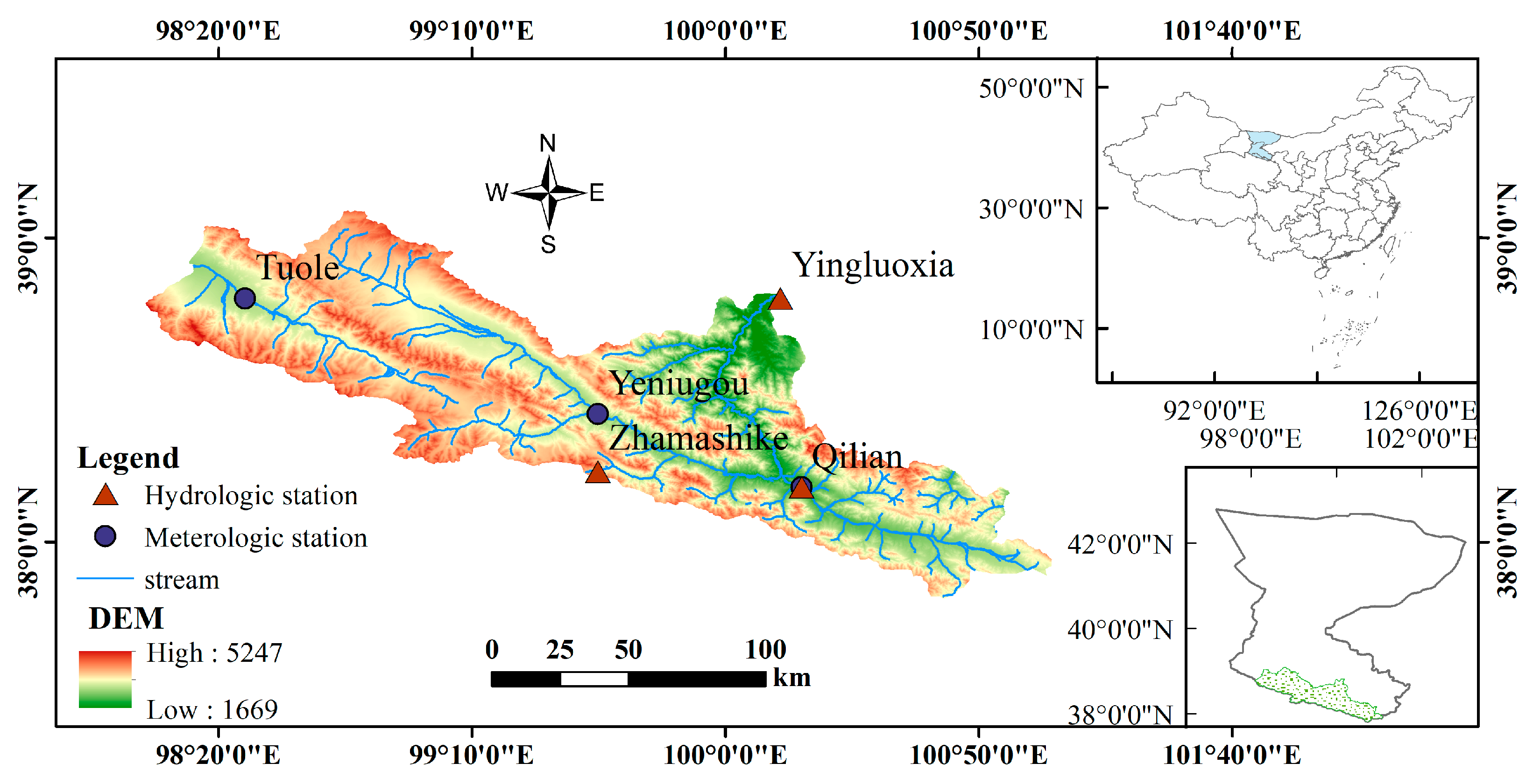
The Heihe River Basin is located in the middle of the Hexi Corridor in northwest China; the upper Heihe River Basin is situated in the Qilian Mountains located in the northeastern part of the Tibetan Plateau. The upper Heihe River Basin covers 10,009 km2 and ranges in elevation from 1669 m to 5247 m. The vegetation distribution shows an evident vertical gradient rule with the increase in altitude. The area is mainly covered by alpine desert glacier, alpine meadow, as well as forest and upland meadow. Additionally, loamy soil dominates in this area, and glaciers are widespread [38]. Due to the arid and semiarid climate, the main runoff in the area is derived from precipitation, melting snow, and melting ice. This area consists of arid and semi–arid regions. Influenced by westerly circulation and the polar cold air mass at middle and high latitudes, the precipitation is concentrated during the Asian Summer Monsoon (ASM) from June to September [39]. The upper reaches of the Heihe river has a typical plateau continental climate, with light recombination, intense evaporation, as well as cold winters and cool summers. The annual average rainfall is between 200 and 600 mm. The annual average temperature is between −5 and 4 °C. The annual average runoff is 15.89 × 10⁸ m3. The annual runoff distribution is mainly concentrated in the flood season from May to October, with runoff from other months accounting for only a small proportion [40]. Precipitation and temperature greatly contributed to the increasing runoff, while glacier melt runoff contributes to less than 10% of the runoff increase [41]. There are few meteorological and hydrological stations in the upper Heihe River Basin, as shown in Figure 1. The Yingluoxia station is located at the upstream exit of the Heihe River Basin, which controls the mountainous watershed runoff. The upper Heihe River Basin provides water resources for the whole Heihe River Basin. The upstream water supply situation directly affects the sustainable development of the socioeconomic and ecological environment in the middle and lower reaches [42]. The “Heihe River 97 water diversion scheme” (97 Water Diversion Scheme) is based on the incoming water of Yingluoxia. Accurate runoff estimation not only promotes the implementation of the 97 Water Diversion Scheme, but is also important for the management of the Heihe water resources.
2.1.2. Data
There are 5 observatories in this area, represented by 3 meteorological stations and 3 hydrological stations. The Qilian station is not only a hydrologic station but also a meteorological station. Monthly runoff data observed at the Yingluoxia hydrologic station were used to represent the runoff of the upper reaches of the Heihe River Basin from 2001 to 2016. The basin–wide rainfall data measurements were aggregated to monthly averages recorded at the Qilian, Zamask, and Yingluoxia stations.
The remotely sensed data include precipitation (P), land surface temperature (LST), evapotranspiration (ET) and NDVI products obtained from GEE from 2001 to 2016. The monthly precipitation data recorded by the Tropical Rainfall Measuring Mission (TRMM3B43) had a spatial resolution of 0.25° and a temporal resolution of 1 month. In the TRMM3B43 products, multiple satellite data of high quality were integrated; this product was widely used in scientific research [43,44]. Some studies have applied the TRMM3B43 dataset for the Tianshan and Qilian mountains [45]. The LST and ET data were calculated using an 8-day Moderate Resolution Imaging Spectroradiometer (MODIS) MOD11A2 and MOD16A2 data and 16-day MOD13A2 NDVI data. The MOD–NDVI data are extremely useful for monitoring vegetation dynamics, and the availability of MOD13A2 data in the Qinghai–Tibet Plateau has been shown in past studies [46,47]. Due to the errors caused by the spatial interpolation of meteorological station data, LST data were used instead of air temperature data [48]. The usability of the MOD–ET data was confirmed by a past study [49] in which the authors claimed that the MODIS–derived global terrestrial ET product can estimate actual ET values with a reasonable accuracy. All the remotely sensed data used in this study are summarized in Table 1.
As there is no clear division rule for datasets, in this study, the data were split into two sets: a training set and a testing set. The data contained in the training set accounted for 75% of the total data. Therefore, the data obtained from 2001 to 2012 were used as the training data and the remaining data from 2013 to 2016 were used as the validation data. For efficient learning, the input variables and output runoff were normalized by their corresponding means and standard deviations. The estimation results reveal the retransformation of the network’s output.
2.1.3. Data Preprocessing
The GEE is used widely in various tasks such as global forest change, global surface water, and crop yield estimation [50]. The remotely sensed data utilized in this study were obtained from the GEE, as this platform can quickly process large images in batches using the online JavaScript application programming interface (API).
Firstly, the vector data for the study area were uploaded into the GEE, and images collected from 2001 to 2016 over the study area were acquired based on GEE. Secondly, the bands of precipitation, NDVI, and ET were selected from theTRMM3B43, MOD16A2, and MOD13A2 products, respectively. All the remote sensing data were clipped to obtain gridded inputs according to the vector data of the study area. The TRMM3B43 dataset had a monthly temporal resolution and did not need to be synthesized. LST data were obtained through averaging the cloud–free pixels of the LST_Day_1km and LST_Night_1km bands over the compositing period. The monthly regional average LST, NDVI, and ET of the study area were calculated according to the MOD11, MOD16A2, and MOD13A2. A reduceRegions() function was then adopted for calculating the spatial mean over the study area for each image. Monthly data for each factor were obtained for used as model inputs. Finally, the values of the P, NDVI, ET, and LST data were exported in the comma–separated values (csv) format. These data from GEE were used to build the model in this study.
2.2. Methodology
2.2.1. LSTM
A recurrent neural network (RNN) is a type of ANN, and the long and short–term memory (LSTM) neural network is a special type of RNN. LSTM is able to solve the gradient explosion and disappearance problems that arise in RNNs, and the LSTM network can also handle complex and long–lag tasks which traditional RNNs cannot handle [15].
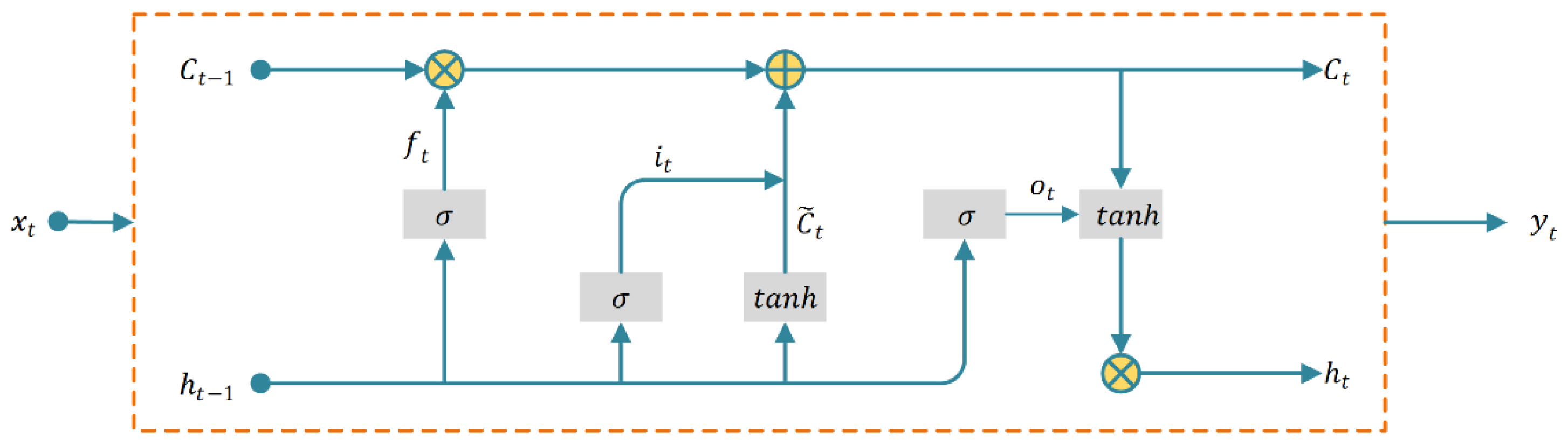
The basic structure of an LSTM cell is shown in Figure 2; in each cell, there are three types of gates that control the flow of information: an input gate, a forget gate, and an output gate. The forget gate is controlled by an activation function such as a Sigmoid or rectified linear unit (ReLU); this function can selectively discard the old cell state Ct−1 information through a calculation using the current input vector xt and previous result ht−1. In the input gate, it is calculated using the activation function with xt and ht−1. A candidate cell state is generated by a tanh layer with xt and ht−1. In addition, the new cell state Ct is updated. The output gate determines the information output from the cell containing and ht, and ht is calculated by output parameter ot and the tanh function of Ct. The calculations performed at every time step of the above process are as follows:
where , , , and are the different weights derived from the forget, input, and output gates; , , and are the corresponding bias values; and , , and are the outputs of the activation function at time t.
2.2.2. Fully Connected LSTM Model
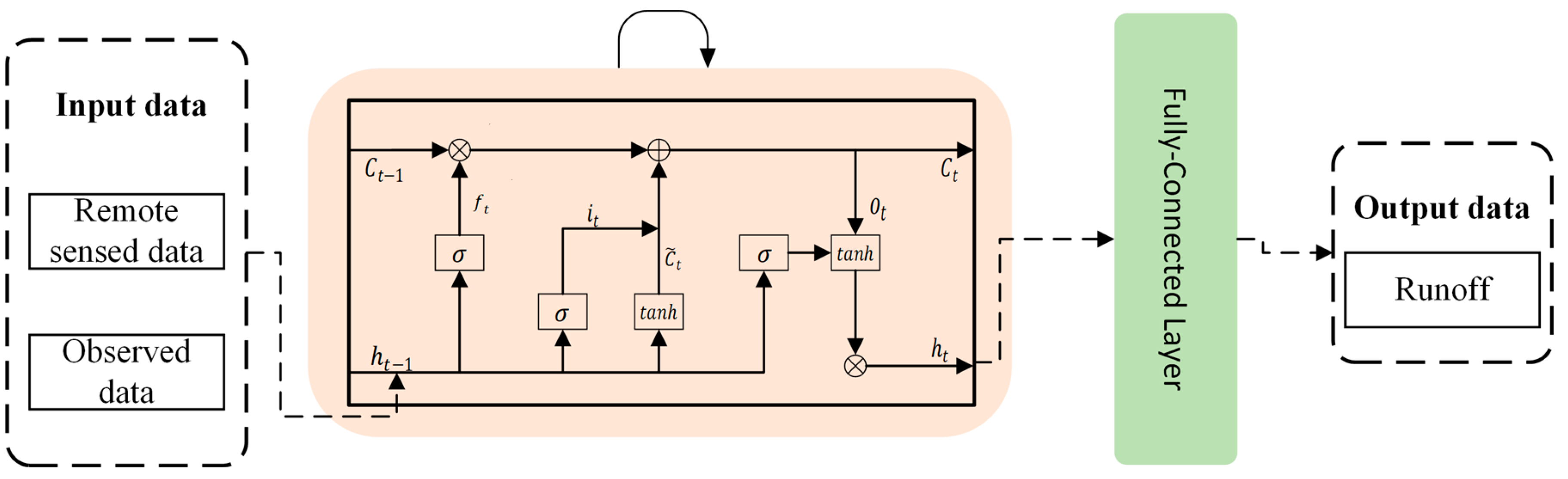
In this study, the fully connected LSTM (FC–LSTM) model was composed of an input layer, an LSTM, a fully connected (FC) layer, and an output layer; the model structure is depicted in Figure 3. The hydrological variables used as inputs were ciphered in the LSTM layer which retained the important information and extracted the nonlinear relations between the variables and runoff. Then, the FC layer received the calculated data and strengthened the fitting ability of the model. Finally, the output layer provided the estimation results.
The selection of input variables is an important step in runoff estimation and has significant influence over the estimation results. Generally, many variables may affect the precipitation–runoff relationship, including precipitation, previous runoff, evaporation, and temperature [51]. To date, many studies on runoff estimation have involved the use of runoff and rainfall as inputs [7,52]. However, other studies have applied evapotranspiration and temperature data as inputs, and these inputs can efficiently improve the performance of the model [53,54,55]. Additionally, the use of NDVI as a biophysical parameter has complex effects on the precipitation–runoff relationship, and some studies have pointed out that the use of NDVI, together with hydroclimatic parameters, can improve the performance of network models [56,57]. Therefore, precipitation, evapotranspiration, temperature, and NDVI were selected as variables in the utilized model. To compare the impacts of different input variables on the estimation results, an input combination was adopted based on the input variables of the model. In addition, P was used as a kind of input. Considering the high correlation between NDVI, precipitation, and runoff, NDVI was used as an input based on P [58,59]. Some studies have claimed that changes in vegetation significantly affect runoff processes by impacting evapotranspiration [60,61]. Therefore, L4 was composed of P, NDVI, and ET. Taking into account the terrain properties of the study area and the complex relationship between LST and runoff, the LST data were used as inputs based on L4. Several combinations of input variables with one set of observation data and three sets of remote sensing data were established:
- L1: P (observed);
- L2: P(RS);
- L3: P(RS), NDVI;
- L4: P(RS), NDVI, ET;
- L5: P(RS), NDVI, ET, LST;
- L6: P(observed), NDVI, ET, LST.
Hyperparameters can directly affect the performance of neural network structures. As there is no standard for the depth or unit number of networks, the trial–and–error method was adopted herein. After many experiments, the best model was set to contain 40 neurons in the LSTM hidden layer. The architectural parameters of the LSTM models have already been extensively tuned by Zhang, J. [21]. Based on the architectures, hyperparameter tuning was performed for the monthly scale model. Three hyperparameters needed to be adjusted (namely training iteration, learning rate, and dropout). Based on the training results obtained for the above combinations, the best configuration with the best R2 value was selected [62]. The number of training iterations was 15,000. The dropout regularization method was used to prohibit overfitting, and the value was set to 0.5. In addition, stochastic gradient descent (SGD) was used to optimize the model parameters and minimize the loss function, and the learning rate was 0.00001. SGD is an optimization algorithm that is widely used in deep learning tasks; it is the central tool used to cope with the approximate solutions of stochastic optimization problems [63].
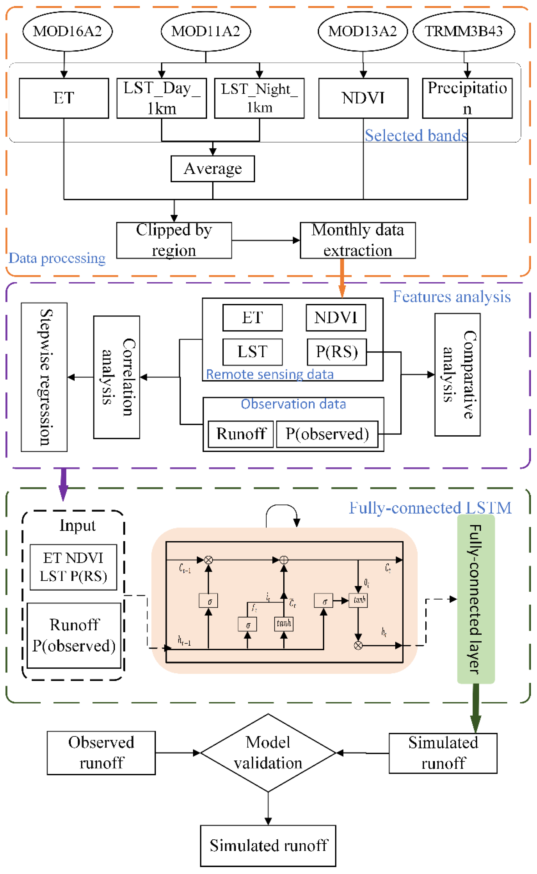
A schematic overview of the study is provided in Figure 4. The flowchart shows the framework of the study including data processing, feature analysis, runoff simulation, and accuracy validation.
2.2.3. Evaluation of Model Performance
Evaluating the model performance is an important component of research. In this study, three methods were employed to evaluate the accuracy of the estimation results: the coefficient of determination(R2), the root mean square error (RMSE) and the Nash–Sutcliffe efficiency (NSE). The RMSE method refers to the deviation of the analogue value from the actual value. The smaller the RMSE value is, the better the estimation process will be. The mathematical formula is shown below:
The R2 method describes the degree to which the model interprets the actual value. R2 values range within the interval of 0–1. The closer the result is to 1, the better the model fitting effect is. The mathematical formula is shown below:
The NSE method is generally used to verify the quality of the hydrological model estimation results, and NSE values fall within the interval of −∞–1. The closer the result is to 1, the better the model fitting effect is. The mathematical formula is shown below:
where is the simulated runoff and yi represents the observed runoff.
3. Results
3.1. Relation of Input Variables and Runoff
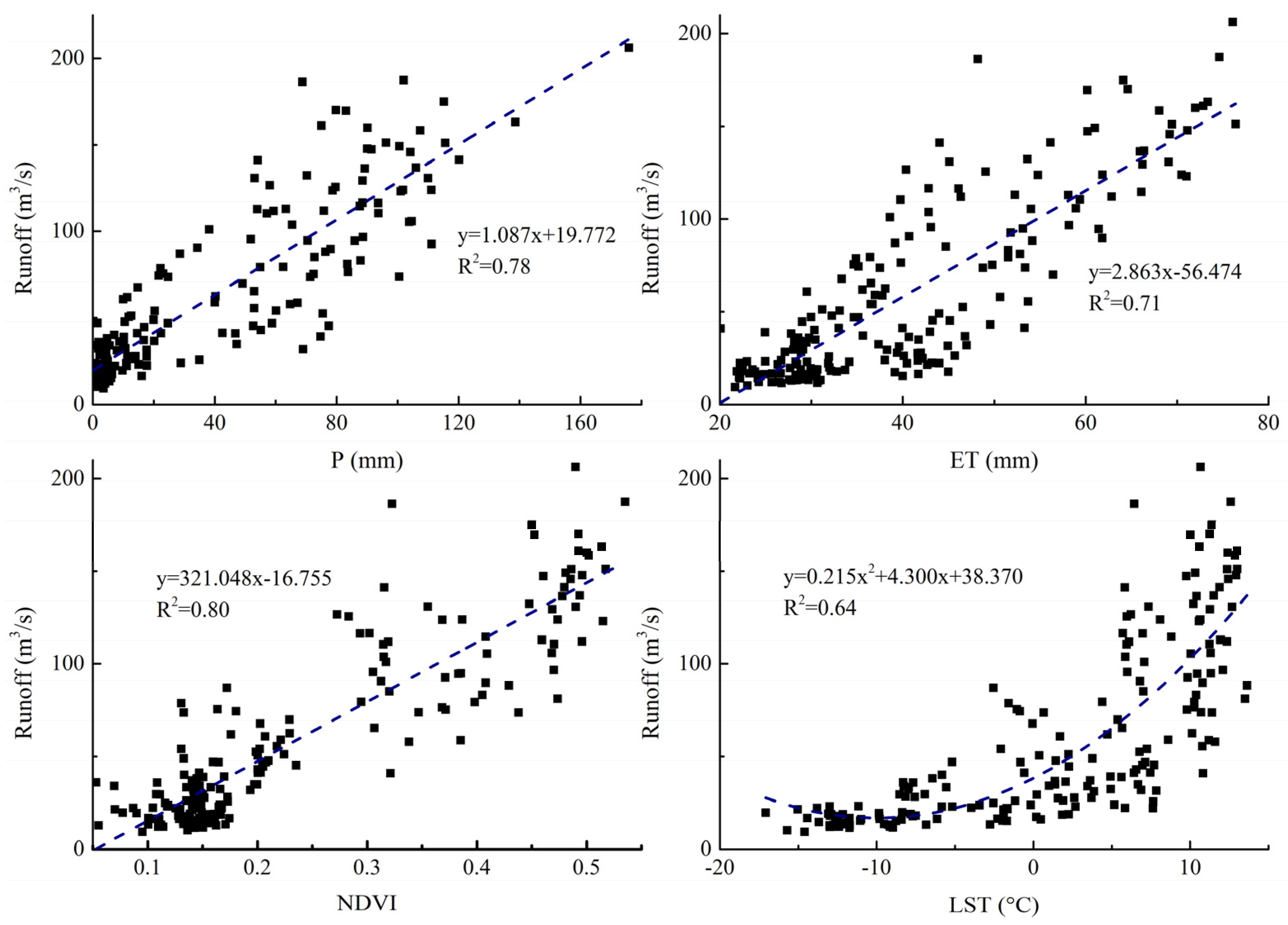
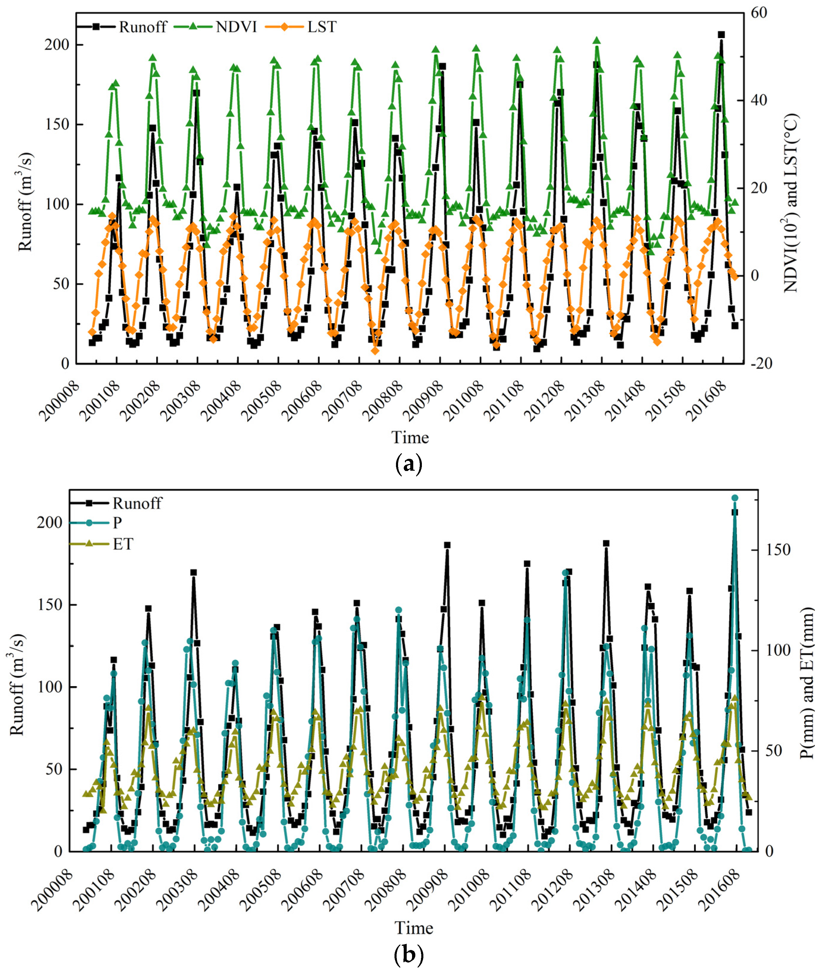
Runoff formation depends on numerous complex factors. In this study, highly correlated factors, such as terrestrial surfaces, vegetation processes, and meteorological parameters were utilized to simulate runoff processes. Four parameters were used to estimate runoff: P(RS), ET, NDVI, and LST. The data were obtained from remote sensing data inversions. Figure 5 shows the relationships existing among P(RS), ET, NDVI, LST, and runoff. The scatter of all variables was linearly positively fitted with that of runoff; among the variables, the relation between LST and runoff was the most complex. As determined from the R2 range of 0.7–0.8, runoff separately showed quite high correlations with the P(RS), ET, and NDVI, but not with the LST. From Figure 6, it can be seen that the change in the oscillation amplitude of LST was slight during the study period, while the response of LST to the runoff dynamics was limited. The LST and runoff had a relatively poor correlation. LST is considered to be the fundamental indicator of climate change, and its feedback to hydrological cycles is complex. The NDVI was the most relevant for runoff with the highest R2 followed by P(RS). As shown in Figure 5, as the peak runoff changed annually, the NDVI, P(RS), and ET respond accordingly. The runoff, NDVI, P(RS), and ET had similar interannual fluctuation patterns, and the change in these four input variables influenced the runoff change; furthermore, these parameters were well synchronized.
Table 2 shows the coefficients of four factors based on stepwise regression by SPSS. Model 1 and model 2 were transitions and model 3 was the final model. In the process of modeling, NDVI was chosen first, followed by P(RS) and ET, while LST was eliminated. In model 3, the sig. of NDVI, P(RS), and ET was less than 0.05 and the three factors had statistical significance. The strength of their linear correlation with runoff decreased sequentially. In addition, the relationship between LST and runoff was found to be more complex. The VIF (variance expansion coefficient) and tolerance value can be used to test the collinearity of the independent variables. The maximum VIF value of the three factors was 6.869. Compared with the collinearity standard value of 10, there was no multicollinearity problem for independent variables. The value obtained from tolerance also supported this phenomenon.
Figure 6 shows the time series of runoff, P(RS), ET and NDVI from 2001 to 2016. There was some periodicity in the temporal fluctuations of runoff during the study period. In addition, the annual runoff showed a slightly increasing trend. The maximum runoff occurred around June each year, while the minimum runoff roughly appeared in January every year. The highest annual runoff value occurred in 2016 at 206.2355 m3/s, while the lowest occurred in 2012 at 9.2581 m3/s. The runoff dynamics changed obviously. The peak runoff rose noticeably from 2009 to 2016 compared to the peak runoff from 2001 to 2008. Similarly, the P(RS), ET, NDVI, and LST dynamics presented 15-year cycles from 2001 to 2016, and their maximum and minimum values appeared roughly at the same time. The peak values always appeared in summer, and the lowest values occurred in winter each year. The trend in each year was consistent with the runoff variations. Generally, the changes in these four variables were highly consistent with those in runoff.
Figure 7 shows the correlation of P(RS) data and rainfall data obtained by observatories. The in situ data used in the model were from three stations in the upper reaches of HRB. In addition, the Qilian station and Zamask station are located upstream of Yingluoxia station. P(RS) represents the precipitation data based on remote sensing technology, while Qilian_P, Zamask_P and Yingluoxia_P refer to the rainfall data from the Qilian, Zamask, and Yingluoxia stations. The Pearson correlation coefficient (PCC) measures the linear correlation between variables. The numbers in Figure 7 show the PCC among the precipitation data from different sources. Values greater than 0.8 indicate strong positive correlations between P(RS) and in situ rainfall data. The value of PCC between P(RS) and the precipitation data from Qilian station and Zamask station was close to 1. A correlation coefficient of 1 implies a perfectly linear correlation. Thus, the P(RS) data could be input into the FC–LSTM model as rainfall data.
3.2. Runoff Estimation
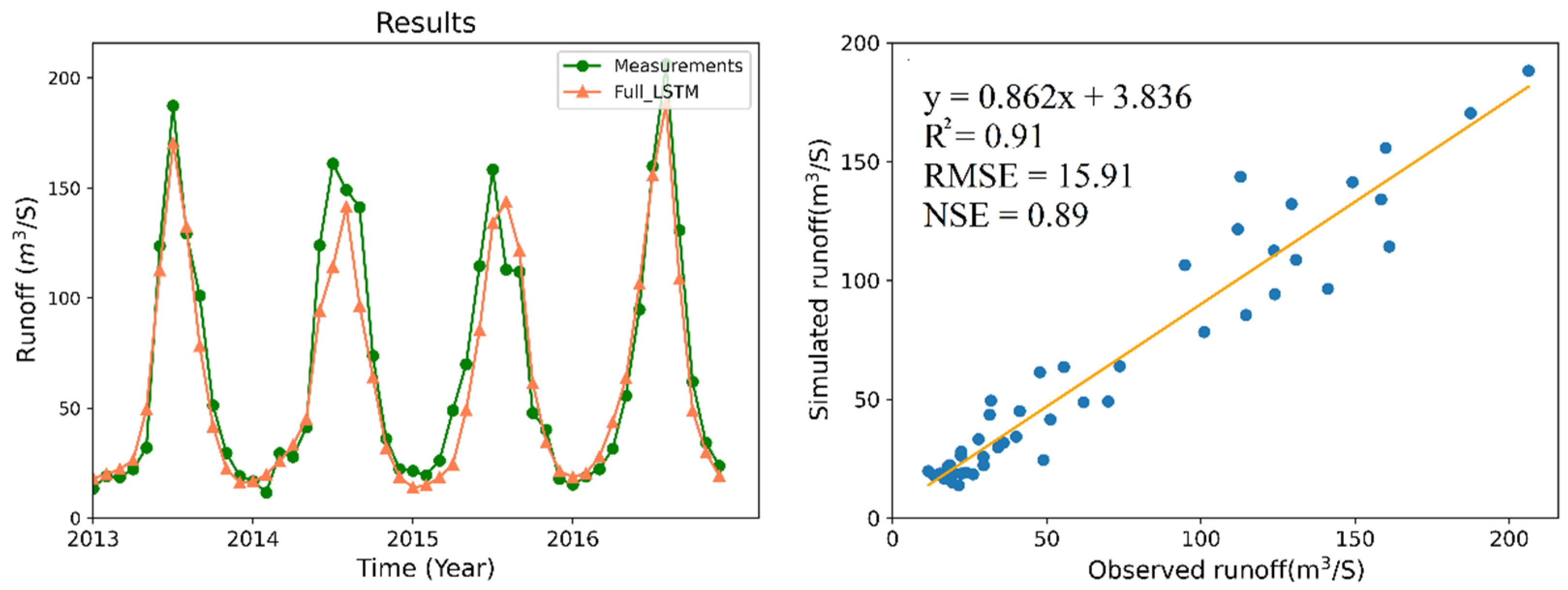
In studies using data–driven methods to estimate runoff, data recorded by meteorological and hydrological stations are always of high quality. Thus, the accuracy of the estimation results is strongly dependent on the model architecture and setting. The first group, L1, contained the rainfall data observed from three stations and was used to test the performance of the fully connected LSTM model. Figure 8 shows the calculation results obtained during the verification period. The model can basically reproduce the runoff process, and the simulated runoff was adjacent to the real runoff. According to Table 3, using L1 as the input results in a high R2, NSE values of 0.91 and 0.89, and a low RMSE value of 15.91. Therefore, the model can accurately capture the runoff pattern during the study period and perform well in the study area.
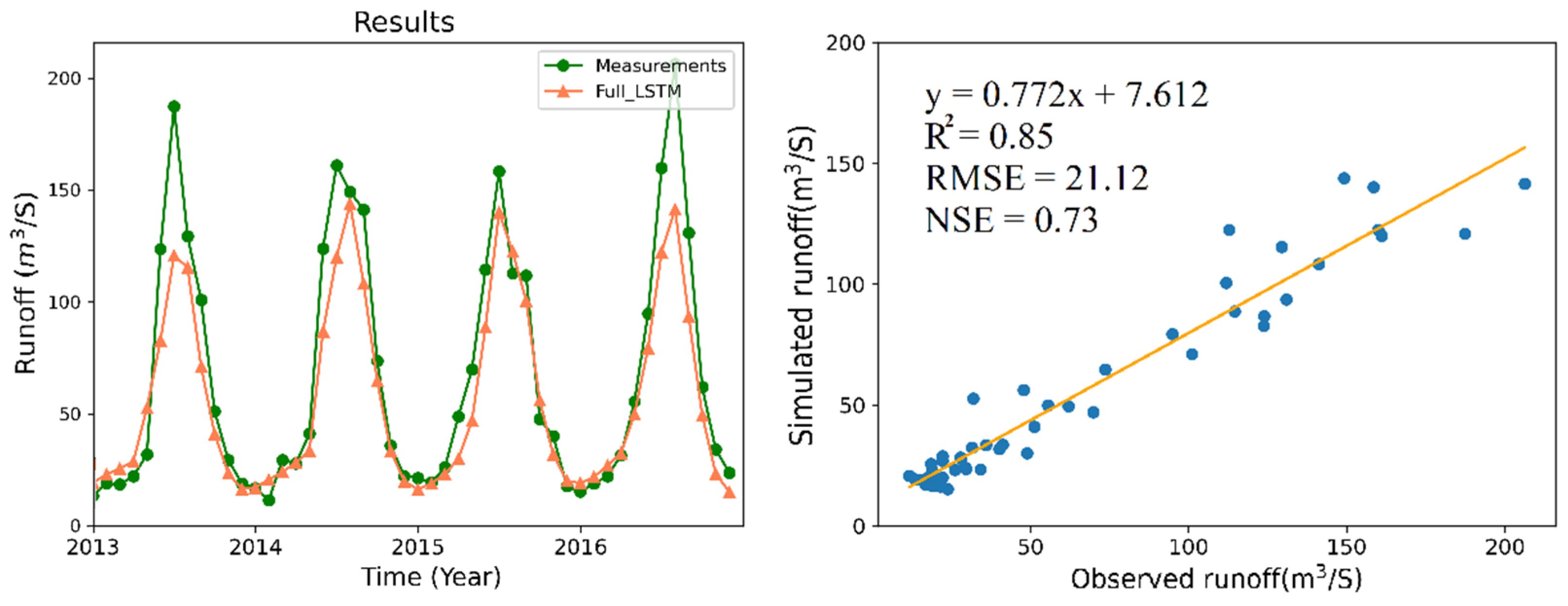
Figure 9 shows the model estimation results obtained under L2, in which P(RS) data were incorporated. With the good performance of the model under L1, the remote sensing data were preliminarily evaluated under the L2 inputs. Figure 9 shows that the simulated hydrograph fits the general trends of the hydrograph and that the estimations of low values were more accurate than those of high values. However, the performance deteriorates compared to the results obtained when using L1 as the input as the R2 and NSE values decrease to 0.85 and 0.73, respectively, and the RMSE value increases to 21.12. Although the performance of the L2 inputs was slightly worse than that of the L1 inputs, the statistical indices showed good results. Considering the important role of vegetation information in rainfall runoff processes, the use of NDVI as a vegetation parameter is critical among input variables [60].
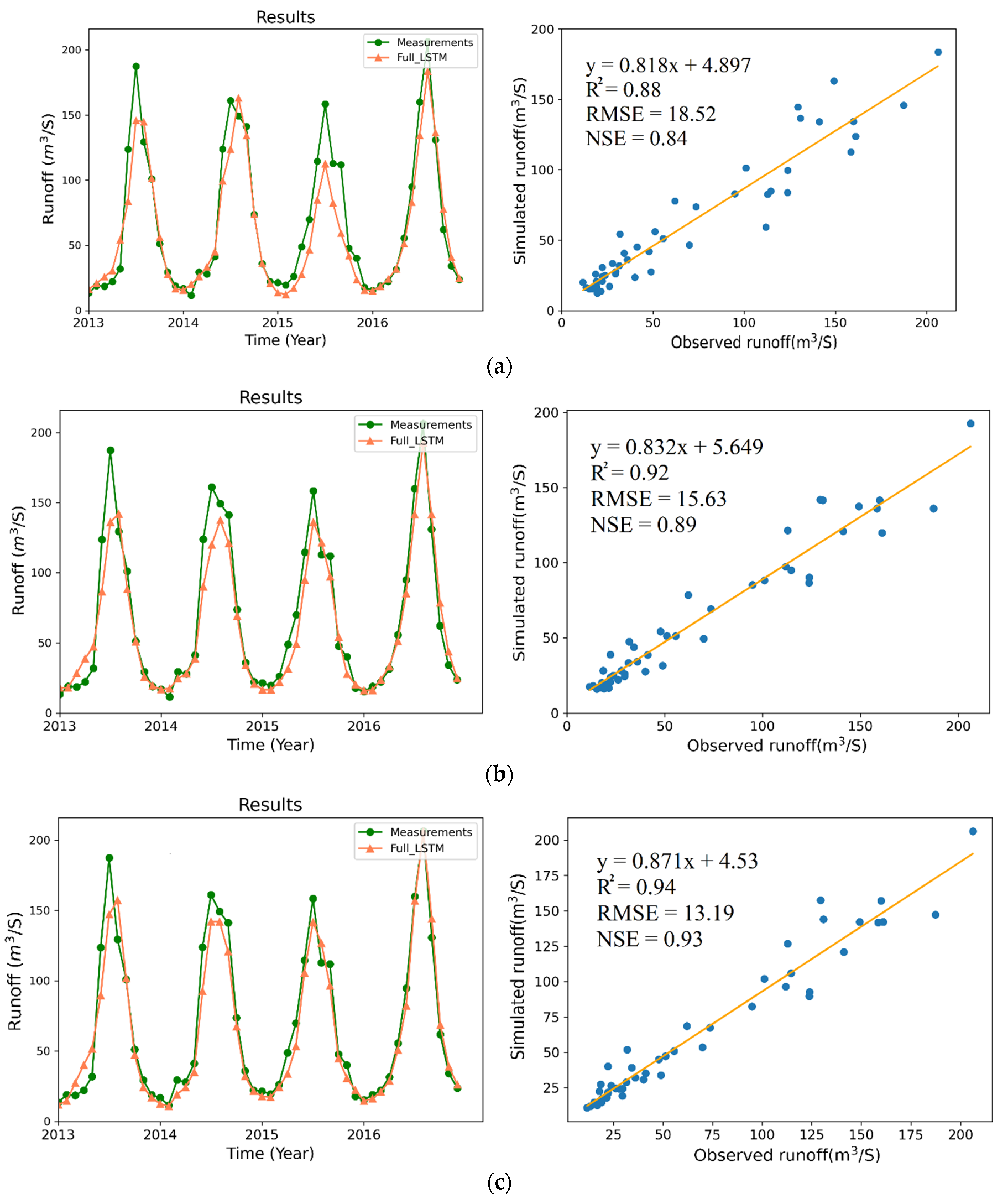
As illustrated in Figure 10a, the runoff can be simulated precisely in several months every year when L3 is used as an input. The R2, RMSE, and NSE values obtained for the model under L3 were better than those obtained under L2. The hydrograph trends were described well in 2016, while in 2015, the performance was unsatisfactory. Similarly, the model simulations were unable to grasp the extreme peak runoff values, which always occur in concentrated periods of rain. When L4 was used as the model input (Figure 10b), the difference between the simulated hydrograph and modeled hydrograph was further narrowed. The R2 value exceeded 0.91 under L4 which was greater than R2 under L1, and the RMSE value was also lower than that derived under L1. The NSE value was improved relative to that determined when L3 was used. In addition, the estimations derived for 2015 were more accurate than those obtained for other years. Thus, the inclusion of ET could efficiently improve the performance of the model. However, there was no significant promotion of the straight line’s slope in the scatter plots. Table 3 shows that the R2, RMSE, and NSE values were 0.94, 13.19, and 0.93, respectively. Among all combinations, the performance of the model was the best when L5 was used as the input (Figure 10c). The evaluation indices of L5 were significantly different under other inputs. The straight line’s slope was the closest to 1, meaning that the simulated results approached the observed values.
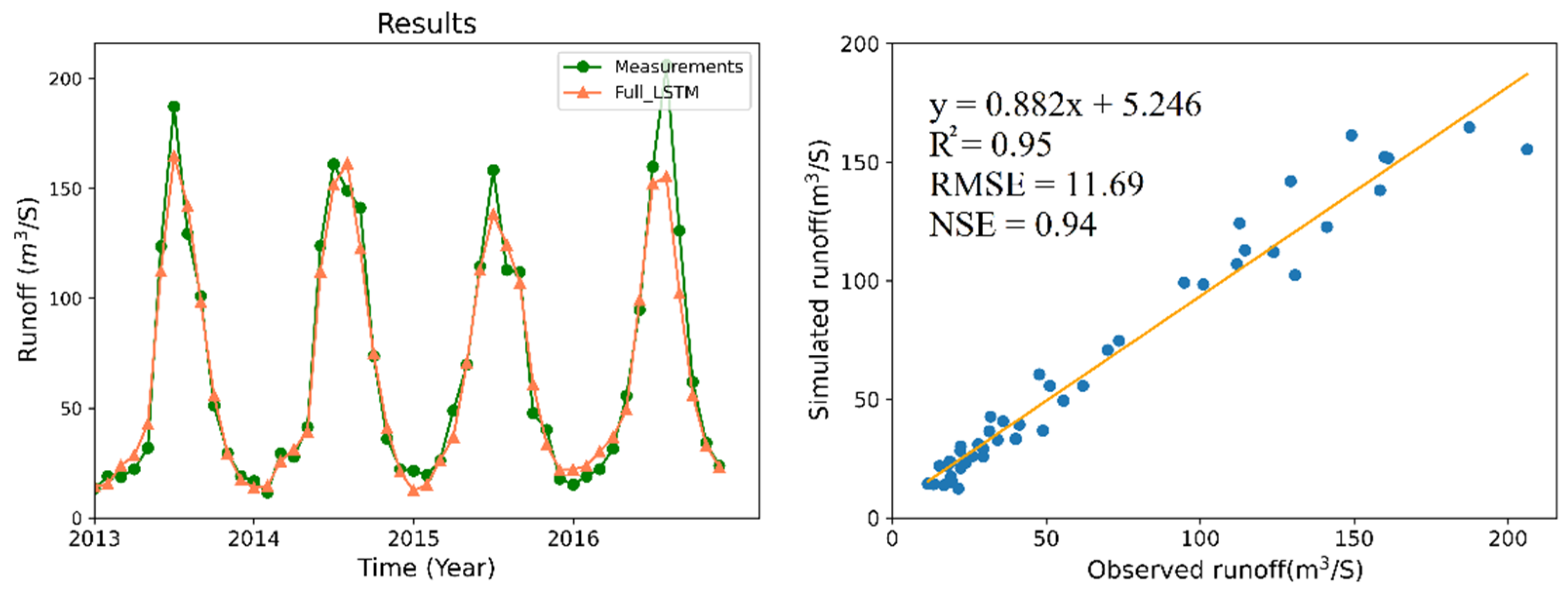
With the incorporation of the in situ data based on L5, the model showed a more accurate performance. The estimation results show hysteresis in 2015 with L1, L2, L3, and L4 as input. Additionally, the incorporation of ET led to the estimation of the hysteresis. Compared to the results obtained under L5, the R2 and NSE evaluation indices slightly increased to 0.95 and 0.94, respectively. Whereas the estimation skill increased quite steeply from L1 (Figure 8) to L6 (Figure 11), the improvement was indicated by a noticeable increase (4–5%) in the R2 and NSE values of runoff and a significant decrease (up to 4.22) in the RMSE value. The comparisons made between L5 and L6 showed that the incorporation of in situ rainfall data slightly improved the performance of the model. Thus, the precipitation data obtained from remote sensing technology provide an alternative way to estimate runoff without observed data. These results indicate that remote sensing technology can play a major role in improving runoff estimates in ungauged basins.
The scatter plots in Figure 8, Figure 9, Figure 10 and Figure 11 show similar patterns and a dividing line can be seen when the runoff value is 100 m3/s. When the values are less than 100 m3/s, the points present a tight distribution around the straight line. However, the points are more dispersed when the values are greater than 100 m3/s. Combined with the corresponding line graphs, low runoff values always occur in winter from the November of a given year to the February of the following year. High values appeared in summer and autumn from June to September. Obviously, the model precisely simulated runoff in winter, but there was room for improvement when simulating summertime runoff. There was a margin of error in simulating springtime runoff from March to May. This uncertainty might be attributed to glaciers and snow cover in the upper Heihe River Basin. Snowmelt has the greatest impact on runoff from March to July [64] and rainfall is concentrated in the summer and autumn. These factors restricted the prediction accuracy of the model in the peak flow season. In addition, the model performed especially unstably in 2016 in the peak runoff season. Combined with Figure 5, the precipitation that occurred in the ASM season in 2016 was significantly higher than in previous years, making it difficult for the model to carry out an accurate simulation.
Table 3 presents the performance indices derived in the runoff simulations under six combinations of input variables. The model showed good results when the L1 set was used as input, and the accuracy decreased when remotely sensed precipitation data were used, with the R2 value being reduced by 0.06. As NDVI and ET were added as input data, the simulation accuracy improved and surpassed that of L1. As more remote sensing variables were included as inputs, the model began to provide more precise results. With the same model architecture, the model could simulate runoff under L6 with the best efficiency through the use of both in situ data and satellite–based data. In particular, the simulation accuracy was dramatically improved compared to that of L1. These results indicated that remote sensing data could efficiently help the model capture monthly runoff fluctuations. In the process of runoff formation, in addition to precipitation, other factors played important roles in the formation process; in this study, ET was used as the soil feature, NDVI was set as a biophysical parameter, and LST was used as a climate factor.
4. Discussion
Many studies have shown that the LSTM network has great potential for obtaining hydrological estimations. In combination with other networks, LSTM has been widely used in hydrological studies. Zhang J. et al. [21] proved the strong learning ability of the fully connected LSTM when using time series data. In this study, the fully connected LSTM model was used as a rainfall–runoff model to obtain runoff estimations. The model verifications indicated that the model could achieve good accuracy when simulating monthly runoff in the upstream reaches of the HRB (Table 3). In the upstream area of the HRB, many studies achieved satisfactory results in runoff estimation [3,65,66]. Teng F. et al. [36] applied a Precipitation–Runoff Modeling System (PRMS) to simulate rainfall runoff in the Zamask–Yingluoxia subbasin of HRB with NSE = 0.90. Zou S. et al. [3] integrated a coupled climate hydrological RIEMS–SWAT model to simulate monthly runoff in the upper reaches of the HBR with the best R2 = 0.83. However, the estimation accuracy obtained based on the physical model was still lower than that found in this study. In addition, the excessive demands of the physical model highlight the advantages of the FC–LSTM network. Therefore, this powerful, fully connected LSTM model could flexibly extract the complex relevant information of various parameters and runoff when handling temporal correlation. Liu D. et al. [67] compared the performance of the Vanilla LSTM, Stacked LSTM, and EMD–En–De–LSTM in a streamflow simulation; their results showed that their reliability gradually increased with the best R2 = 0.93. In addition, compared to the performance of the vanilla LSTM, the FC layer efficiently improved the simulation accuracy and FC–LSTM outperformed EMD–En–De–LSTM in the simulation of runoff. Yuan X. et al. [68] showed the high accuracy of hybrid long short–term memory neural network and ant lion optimizer model (LSTM–ALO) for the prediction of monthly runoff with an R2 = 0.948. The ALO was utilized to optimize the number of hidden layers and update the learning rate. The two parameters used in this study were set using the trial–and–error method. The FC–LSTM model might be able to be further improved by adding an optimizer. Generally, the model used herein served as a useful tool for providing scientific support and water resource management guidance. This model is of great significance to the sustainable development of the study region.
In runoff estimations, input data have a critical influence on the estimation result. Most data were obtained from meteorological observatories and hydrological stations [65,68,69]. However, some regions with hydrological stations do not have meteorological stations. In some areas, due to the limitations of regional development, the number of in situ stations has decreased over a lengthy period. Additionally, there are some areas where data for meteorological and hydrological stations are available, but the stations are scarce or unevenly distributed. Currently, the hydrological models including physical based models and data–driven models to obtain runoff estimations should be driven by sufficient data, but these data are difficult to obtain in the aforementioned areas [3,66]. In these cases, remote sensing data provide a reliable means for runoff estimation. In this study, precipitation data obtained from observatories and satellite had high consistency (Figure 6). The model that used P(RS) as an input had a good performance. In the absence of environmental data and meteorological data for the stations, the model that used runoff data and satellite data as the input achieved high accuracy with R2 = 0.95. Satellite data provide temporally and spatially dynamic information on underlying surface variations. Missing observatory data can be compensated for by applying the information derived using remote sensing techniques. In many previous studies, applications of remote sensing data for runoff estimations have performed well [70,71,72]. In this study, the remote sensing data were processed without taking into account the impact of different spatial resolutions. Choi H.I. [73] found that the performance of a finer resolution result in runoff prediction is much better than that of a coarser resolution result. Thus, this model may be further improved by considering spatial resolution. Simulating runoff in areas with insufficient hydrological data is a challenging aspect of hydrological research. Remote sensing data products provide another method for obtaining hydrological and other forms of relevant data and could be used as an alternative means to simulate runoff in areas lacking data.
Some studies have claimed that the use of ET or temperature as the input variable may lead to worse model performance [74,75]. In this study, the runoff estimation ability of the LSTM model was explored with remote sensing data upstream of the HRB and the influence of various input parameters on the results were analyzed in detail. It is worth noting that the estimation results were better when new parameters were included as input. The estimation results obtained under the L4 input set surpassed those obtained using the observed data. The L6 input set, which included precipitation and other related factors (NDVI, ET and LST) showed the best estimation effect. The amount of relevant data was a significant component affecting the accuracy of the runoff estimation [12]. In the stepwise regression, LST was eliminated from the linear model, while the model with L5 as an input performed better than that with L4. This indicated that LST contributed to the runoff formation. Permafrost, seasonal frozen ground, and glaciers exist in the upper HRB. Yang D. et al. [76] proved that the soil freezing and thawing process significantly influenced the runoff generation in the upper HRB. In the ASM season, the thawing of soil ice together with a large amount of rainfall results in an increase in runoff [39]. The lacking of soil and land use data limited the performance of the model in the peak flow season [77]. With its great performance in snowmelt–driven catchments [10,78], the LSTM–based model might be able to provide a more accurate simulation if snow cover data were used as inputs. In addition, LST might influence the catchment hydrology by significant changing frozen soils. In this study, runoff was found to be affected by the rainfall, NDVI, ET, and LST. Sang Y.-F. et al. [79] found that, at higher temperatures, snow and glacial melt resulting from increasing temperatures and precipitation caused runoff changes in the upper reaches of the Heihe River Basin. As global climate change was confirmed, climate change intensified the hydrological cycle at the global scale. Rainfall, ET, and temperature trends have also changed to varying degrees [80]. A series of consequences resulting from these changes may have direct and dramatic effects on runoff [81]. Many factors affect the formation of runoff. The numerous complex interactions and feedbacks occurring among the precipitation and evapotranspiration processes in the water cycle as well as geophysical characteristics make it difficult to construct a proper model. Under the situation of global climate change, these factors are affected to a certain extent. The interactions between variables and runoff are becoming increasingly complex, placing higher requirements on the ability of models to extract relevant information. In addition, studies estimating river basin runoff must not only consider the parameters related to runoff, but must also take the impacts of regional climate change factors on runoff into consideration.
Generally, the model described in this study showed a tendency to underestimate runoff peaks, which is also a common problem in runoff prediction models [82]. The model needs to be improved to correct this tendency. The study period covered a time span from 2001 to 2016, and the upper HRB was in a high flow period after 2000 with the continuous increase in runoff. The model was applied during the study period. The model‘s performance was not tested in a drought period, and the simulation of longer time series runoff by the model remains to be studied. In addition, high warm humidification tendencies occur in northwest China, with the air temperature, precipitation and near–surface air humidity significantly increasing from 1979 to 2018. In the future, the climate in northwest China will continue to be warm and humid, though climatic factors such as precipitation and humidity will also change [83]. The ability of the model in this scenario remains to be investigated. The upper HRB is located in the central and eastern part of the Qilian Mountains, where the impact of human activities is gradually increasing. Incorporating the effects of climate change and human activities into the model will be carried out in future work.
5. Conclusions
In this study, a fully connected data–driven modeling method was employed in a runoff simulation based on remote sensing data. Before the investigation, the remotely sensed data were preprocessed and downloaded from the GEE, covering the period from 2001 to 2016; the utilized data included the TRMM–P, MOD–NDVI, MOD–ET, and MOD–LST datasets. The rainfall and runoff data were obtained from meteorological and hydrological stations in the upper HRB. The model was used to simulate runoff in the upper Heihe River Basin during the 2013–2016 period using satellite–derived input variables and observed data, respectively, with the data derived over the first 12 years used as the training dataset. The following results were obtained:
- The fully connected LSTM model had an excellent learning capability for simulating runoff and a flexible ability to extract complex relevant information; an R2 value of 0.91 was obtained for the observed data, and a value of 0.95 was obtained for the mixed data.
- It was possible to consider the remotely sensed data as the input data for the model to estimate runoff. The best performance of the model was obtained when the in situ data and remotely sensed data were used together as inputs. Remotely sensed data could thus be an alternative way of supporting runoff forecast experiments in areas lacking meteorological, soil, and geomorphological data;
- It was worth noting that the amount of input data used had a vast influence on the model performance. As the number of input variables increased, the estimation result became more accurate. The input variables were thus strongly correlated with the outputs.
The continuous improvement of remote sensing technology has greatly improved the quality of remote sensing data products and created more opportunities for hydrological research. At the same time, the in–depth and extensive application of deep learning research provides scientific support for the use of water resources. The combined used of remotely sensed data and deep–learning methods to estimate runoff achieved good results, providing a fast and cost–effective solution for estimating runoff in areas lacking hydrological data across the world. Additionally, the proposed method is helpful for water resource management and scientific decision–making in the study region. This study was only conducted on a monthly scale, and runoff simulations on other timescales such as hourly and weekly scales require further study.
Author Contributions
Conceptualization, H.X., G.D. and J.L.; methodology, H.X. and G.D.; software, H.X., J.L., C.Z. and D.J.; validation, H.X., J.L. and C.Z.; formal analysis, J.L., G.D. and J.L.; investigation, H.X., G.D. and J.L.; resources, G.D.; data curation, G.D.; writing—original draft preparation, J.L.; writing—review and editing, J.L., H.X. and G.D.; visualization, J.L. and G.D.; funding acquisition, G.D. and H.X. All authors have read and agreed to the published version of the manuscript.
Funding
This research was funded by National Natural Science Foundation of China, grant number 42061056.
Data Availability Statement
TRMM3B4, MOD12A2, MOD16A2, and MOD13A2 used in this paper can be downloaded from Google Earth Engine. Monthly meteorological and hydrologic data were obtained from the Heihe River Bureau of the Yellow River Conservancy Commission (http://hrb.yrcc.gov.cn/, accessed on 22 March 2022).
Conflicts of Interest
The authors declare no conflict of interest.
References
- Wang, W.C.; Chau, K.W.; Cheng, C.T.; Qiu, L. A comparison of performance of several artificial intelligence methods for forecasting monthly discharge time series. J. Hydrol. 2009, 374, 294–306. [Google Scholar] [CrossRef] [Green Version]
- Zhang, Y.; Chiew, F.H.S.; Zhang, L.; Li, H. Use of Remotely Sensed Actual Evapotranspiration to Improve Rainfall-Runoff Modeling in Southeast Australia. J. Hydrometeorol. 2009, 10, 969–980. [Google Scholar] [CrossRef]
- Zou, S.; Ruan, H.; Lu, Z.; Yang, D.; Xiong, Z.; Yin, Z. Runoff Simulation in the Upper Reaches of Heihe River Basin Based on the RIEMS-SWAT Model. Water 2016, 8, 455. [Google Scholar] [CrossRef] [Green Version]
- Jeong, D.I.; Kim, Y.O. Rainfall-runoff models using artificial neural networks for ensemble streamflow prediction. Hydrol. Process. 2005, 19, 3819–3835. [Google Scholar] [CrossRef]
- Sivapalan, M.; Takeuchi, K.; Franks, S.W.; Gupta, V.K.; Karambiri, H.; Lakshmi, V.; Liang, X.; McDonnell, J.J.; Mendiondo, E.M.; O’Connell, P.E.; et al. IAHS decade on Predictions in Ungauged Basins (PUB), 2003-2012: Shaping an exciting future for the hydrological sciences. Hydrol. Sci. J. 2003, 48, 857–880. [Google Scholar] [CrossRef] [Green Version]
- Yang, W.C.; Jin, F.M.; Si, Y.J.; Li, Z. Runoff change controlled by combined effects of multiple environmental factors in a headwater catchment with cold and arid climate in northwest China. Sci. Total Environ. 2021, 756, 143955–143985. [Google Scholar] [CrossRef]
- Van, S.P.; Le, H.M.; Thanh, D.V.; Dang, T.D.; Loc, H.H.; Anh, D.T. Deep learning convolutional neural network in rainfall–runoff modelling. J. Hydroinform. 2020, 22, 541–561. [Google Scholar] [CrossRef]
- Li, C.; Zhu, L.; He, Z.; Gao, H.; Yang, Y.; Yao, D.; Qu, X. Runoff Prediction Method Based on Adaptive Elman Neural Network. Water 2019, 11, 1113. [Google Scholar] [CrossRef] [Green Version]
- Young, C.-C.; Liu, W.-C. Prediction and modelling of rainfall-runoff during typhoon events using a physically-based and artificial neural network hybrid model. Hydrol. Sci. J. 2015, 60, 2102–2116. [Google Scholar] [CrossRef]
- Kratzert, F.; Klotz, D.; Brenner, C.; Schulz, K.; Herrnegger, M. Rainfall-runoff modelling using Long Short-Term Memory (LSTM) networks. Hydrol. Earth Syst. Sci. 2018, 22, 6005–6022. [Google Scholar] [CrossRef] [Green Version]
- Young, C.C.; Liu, W.C.; Wu, M.C. A physically based and machine learning hybrid approach for accurate rainfall-runoff modeling during extreme typhoon events. Appl. Soft Comput. J. 2017, 53, 205–216. [Google Scholar] [CrossRef]
- Liu, Y.; Zhang, T.; Kang, A.; Li, J.; Lei, X. Research on Runoff Simulations Using Deep-Learning Methods. Sustainability 2021, 13, 1336. [Google Scholar] [CrossRef]
- Kumar, D.N.; Raju, K.S.; Sathish, T. River Flow Forecasting using Recurrent Neural Networks. Water Resour. Manag. 2004, 18, 143–161. [Google Scholar] [CrossRef]
- Zhao, R.; Yan, R.; Chen, Z.; Mao, K.; Wang, P.; Gao, R.X. Deep learning and its applications to machine health monitoring. Mech. Syst. Signal Process. 2019, 115, 213–237. [Google Scholar] [CrossRef]
- Hochreiter, S.; Schmidhuber, J. Long Short-Term Memory. Neural Comput. 1997, 9, 1735–1780. [Google Scholar] [CrossRef]
- Tian, Y.; Xu, Y.-P.; Yang, Z.; Wang, G.; Zhu, Q. Integration of a Parsimonious Hydrological Model with Recurrent Neural Networks for Improved Streamflow Forecasting. Water 2018, 10, 1655. [Google Scholar] [CrossRef] [Green Version]
- Fan, H.; Jiang, M.; Xu, L.; Zhu, H.; Cheng, J.; Jiang, J. Comparison of Long Short Term Memory Networks and the Hydrological Model in Runoff Simulation. Water 2020, 12, 175. [Google Scholar] [CrossRef] [Green Version]
- Li, W.; Kiaghadi, A.; Dawson, C. High temporal resolution rainfall-runoff modeling using long-short-term-memory (LSTM) networks. Neural Comput. Appl. 2021, 33, 1261–1278. [Google Scholar] [CrossRef]
- Zhang, Z.; Lv, Z.; Gan, C.; Zhu, Q. Human action recognition using convolutional LSTM and fully-connected LSTM with different attentions. Neurocomputing 2020, 410, 304–316. [Google Scholar] [CrossRef]
- Kratzert, F.; Klotz, D.; Hochreiter, S.; Nearing, G.S. A note on leveraging synergy in multiple meteorological data sets with deep learning for rainfall-runoff modeling. Hydrol. Earth Syst. Sci. 2021, 25, 2685–2703. [Google Scholar] [CrossRef]
- Zhang, J.; Zhu, Y.; Zhang, X.; Ye, M.; Yang, J. Developing a Long Short-Term Memory (LSTM) based model for predicting water table depth in agricultural areas. J. Hydrol. 2018, 561, 918–929. [Google Scholar] [CrossRef]
- Xu, W.; Jiang, Y.; Zhang, X.; Li, Y.; Zhang, R.; Fu, G. Using long short-term memory networks for river flow prediction. Hydrol. Res. 2020, 51, 1358–1376. [Google Scholar] [CrossRef]
- Rathor, S.; Agrawal, S. A robust model for domain recognition of acoustic communication using Bidirectional LSTM and deep neural network. Neural Comput. Appl. 2021, 33, 11223–11232. [Google Scholar] [CrossRef]
- Sirisena, T.A.J.G.; Maskey, S.; Ranasinghe, R. Hydrological Model Calibration with Streamflow and Remote Sensing Based Evapotranspiration Data in a Data Poor Basin. Remote Sens. 2020, 12, 3768. [Google Scholar] [CrossRef]
- Bugan, R.; Luis Garcia, C.; Jovanovic, N.; Teich, I.; Fink, M.; Dzikiti, S. Estimating evapotranspiration in a semi-arid catchment: A comparison of hydrological modelling and remote-sensing approaches. Water SA 2020, 46, 158–170. [Google Scholar]
- Wigmosta, M.S.; Vail, L.W.; Lettenmaier, D.P. A distributed hydrology-vegetation model for complex terrain. Water Resour. Res. 1994, 30, 1665–1679. [Google Scholar] [CrossRef]
- Huang, Q.; Qin, G.; Zhang, Y.; Tang, Q.; Liu, C.; Xia, J.; Chiew, F.H.S.; Post, D. Using Remote Sensing Data-Based Hydrological Model Calibrations for Predicting Runoff in Ungauged or Poorly Gauged Catchments. Water Resour. Res. 2020, 56, e2020WR028205. [Google Scholar] [CrossRef]
- Beck, H.E.; Vergopolan, N.; Pan, M.; Levizzani, V.; van Dijk, A.I.J.M.; Weedon, G.P.; Brocca, L.; Pappenberger, F.; Huffman, G.J.; Wood, E.F. Global-scale evaluation of 22 precipitation datasets using gauge observations and hydrological modeling. Hydrol. Earth Syst. Sci. 2017, 21, 6201–6217. [Google Scholar] [CrossRef] [Green Version]
- Capolongo, D.; Refice, A.; Bocchiola, D.; D’Addabbo, A.; Vouvalidis, K.; Soncini, A.; Zingaro, M.; Bovenga, F.; Stamatopoulos, L. Coupling multitemporal remote sensing with geomorphology and hydrological modeling for post flood recovery in the Strymonas dammed river basin (Greece). Sci. Total Environ. 2019, 651, 1958–1968. [Google Scholar] [CrossRef]
- Quang, N.H.; Tuan, V.A.; Hang, L.T.T.; Hung, N.M.; The, D.T.; Dieu, D.T.; Anh, N.D.; Hackney, C.R. Hydrological/Hydraulic Modeling-Based Thresholding of Multi SAR Remote Sensing Data for Flood Monitoring in Regions of the Vietnamese Lower Mekong River Basin. Water 2020, 12, 71. [Google Scholar] [CrossRef] [Green Version]
- Zhou, H.; Luo, Z.; Tangdamrongsub, N.; Zhou, Z.; He, L.; Xu, C.; Li, Q.; Wu, Y. Identifying Flood Events over the Poyang Lake Basin Using Multiple Satellite Remote Sensing Observations, Hydrological Models and In Situ Data. Remote Sens. 2018, 10, 713. [Google Scholar] [CrossRef] [Green Version]
- Kwon, M.; Kwon, H.-H.; Han, D. A Hybrid Approach Combining Conceptual Hydrological Models, Support Vector Machines and Remote Sensing Data for Rainfall-Runoff Modeling. Remote Sens. 2020, 12, 1081. [Google Scholar] [CrossRef]
- Jodar, J.; Carpintero, E.; Martos-Rosillo, S.; Ruiz-Constan, A.; Marin-Lechado, C.; Cabrera-Arrabal, J.A.; Navarrete-Mazariegos, E.; Gonzalez-Ramon, A.; Lamban, L.J.; Herrera, C.; et al. Combination of lumped hydrological and remote-sensing models to evaluate water resources in a semi-arid high altitude ungauged watershed of Sierra Nevada (Southern Spain). Sci. Total Environ. 2018, 625, 285–300. [Google Scholar] [CrossRef]
- Li, Z.; Li, Q.; Wang, J.; Feng, Y.; Shao, Q. Impacts of projected climate change on runoff in upper reach of Heihe River basin using climate elasticity method and GCMs. Sci. Total Environ. 2020, 716, 137072. [Google Scholar] [CrossRef]
- Luo, K.; Tao, F.; Deng, X.; Moiwo, J.P. Changes in potential evapotranspiration and surface runoff in 1981-2010 and the driving factors in Upper Heihe River Basin in Northwest China. Hydrol. Process. 2017, 31, 90–103. [Google Scholar] [CrossRef]
- Teng, F.; Huang, W.; Cai, Y.; Zheng, C.; Zou, S. Application of Hydrological Model PRMS to Simulate Daily Rainfall Runoff in Zamask-Yingluoxia Subbasin of the Heihe River Basin. Water 2017, 9, 769. [Google Scholar] [CrossRef] [Green Version]
- Liu, P. A survey of remote-sensing big data. Front. Environ. Sci. 2015, 3, 45. [Google Scholar] [CrossRef] [Green Version]
- Zhang, L.; Su, F.; Yang, D.; Hao, Z.; Tong, K. Discharge regime and simulation for the upstream of major rivers over Tibetan Plateau. J. Geophys. Res. Atmos. 2013, 118, 8500–8518. [Google Scholar] [CrossRef]
- Zheng, D.; van der Velde, R.; Su, Z.; Wen, J.; Wang, X.; Yang, K. Impact of soil freeze-thaw mechanism on the runoff dynamics of two Tibetan rivers. J. Hydrol. 2018, 563, 382–394. [Google Scholar] [CrossRef]
- Yang, M.; Zhang, B.; Wang, H.; Yuan, J. The study on the change of mountainous runoff Heihe River basin from 1950 to 2004. Resour. Sci. 2009, 31, 413–419. [Google Scholar]
- Wang, Y.; Yang, D.; Lei, H.; Yang, H. Impact of cryosphere hydrological processes on the river runoff in the upper reaches of Heihe River. J. Hydraul. Eng. 2015, 46, 1064–1071. [Google Scholar]
- Shang, X.; Jiang, X.; Jia, R.; Wei, C. Land Use and Climate Change Effects on Surface Runoff Variations in the Upper Heihe River Basin. Water 2019, 11, 344. [Google Scholar] [CrossRef] [Green Version]
- Tao, H.; Fischer, T.; Zeng, Y.; Fraedrich, K. Evaluation of TRMM 3B43 Precipitation Data for Drought Monitoring in Jiangsu Province, China. Water 2016, 8, 221. [Google Scholar] [CrossRef] [Green Version]
- Ji, X.; Chen, Y. Characterizing spatial patterns of precipitation based on corrected TRMM B-3(43) data over the mid Tianshan Mountains of China. J. Mt. Sci. 2012, 9, 628–645. [Google Scholar] [CrossRef]
- Liu, J.F.; Chen, R.S.; Qin, W.W.; Yang, Y. Study on the vertical distribution of precipitation in mountainous regions using TRMM data. Adv. Water. Sci. 2011, 22, 447–454. [Google Scholar]
- Du, J.-Q.; Shu, J.-M.; Wang, Y.-H.; Li, Y.-C.; Zhang, L.-B.; Guo, Y. Comparison of GIMMS and MODIS normalized vegetation index composite data for Qing-Hai-Tibet Plateau. J. Appl. Ecol. 2014, 25, 533–544. [Google Scholar]
- Zhu, Y.X.; Zhang, Y.J.; Zu, J.X.; Che, B.; Tang, Z.; Cong, N.; Li, J.X.; Chen, N. Performance evaluation of GIMMS NDVI based on MODIS NDVI and SPOT NDVI data. J. Appl. Ecol. 2019, 30, 536–544. [Google Scholar]
- Liu, Z.; Wang, H.; Li, N.; Zhu, J.; Pan, Z.; Qin, F. Spatial and Temporal Characteristics and Driving Forces of Vegetation Changes in the Huaihe River Basin from 2003 to 2018. Sustainability 2020, 12, 2198. [Google Scholar] [CrossRef] [Green Version]
- Kim, H.W.; Hwang, K.; Mu, Q.; Lee, S.O.; Choi, M. Validation of MODIS 16 global terrestrial evapotranspiration products in various climates and land cover types in Asia. KSCE J. Civ. Eng. 2012, 16, 229–238. [Google Scholar] [CrossRef]
- Gorelick, N.; Hancher, M.; Dixon, M.; Ilyushchenko, S.; Thau, D.; Moore, R. Google Earth Engine: Planetary-scale geospatial analysis for everyone. Remote Sens. Environ. 2017, 202, 18–27. [Google Scholar] [CrossRef]
- Wu, C.L.; Chau, K.W. Rainfall–runoff modeling using artificial neural network coupled with singular spectrum analysis. J. Hydrol. 2011, 399, 394–409. [Google Scholar] [CrossRef] [Green Version]
- Gao, S.; Huang, Y.; Zhang, S.; Han, J.; Wang, G.; Zhang, M.; Lin, Q. Short-term runoff prediction with GRU and LSTM networks without requiring time step optimization during sample generation. J. Hydrol. 2020, 589, 125188. [Google Scholar] [CrossRef]
- Xiang, Z.; Yan, J.; Demir, I. A Rainfall-Runoff Model With LSTM-Based Sequence-to-Sequence Learning. Water Resour. Res. 2020, 56, e2019WR025326. [Google Scholar] [CrossRef]
- Gui, Z.; Liu, P.; Cheng, L.; Guo, S.; Wang, H.; Zhang, L. Improving Runoff Prediction Using Remotely Sensed Actual Evapotranspiration during Rainless Periods. J. Hydrol. Eng. 2019, 24, 04019050. [Google Scholar] [CrossRef]
- Zhang, Y.; Chiew, F.H.S.; Liu, C.; Tang, Q.; Xia, J.; Tian, J.; Kong, D.; Li, C. Can Remotely Sensed Actual Evapotranspiration Facilitate Hydrological Prediction in Ungauged Regions Without Runoff Calibration? Water Resour. Res. 2020, 56, e2019WR026236. [Google Scholar] [CrossRef]
- Asadi, H.; Shahedi, K.; Jarihani, B.; Sidle, R.C. Rainfall-Runoff Modelling Using Hydrological Connectivity Index and Artificial Neural Network Approach. Water 2019, 11, 212. [Google Scholar] [CrossRef] [Green Version]
- Soltani, K.; Ebtehaj, I.; Amiri, A.; Azari, A.; Gharabaghi, B.; Bonakdari, H. Mapping the spatial and temporal variability of flood susceptibility using remotely sensed normalized difference vegetation index and the forecasted changes in the future. Sci. Total Environ. 2021, 770, 145288. [Google Scholar] [CrossRef]
- Schmidt, H.; Karnieli, A. Remote sensing of the seasonal variability of vegetation in a semi-arid environment. J. Arid Environ. 2000, 45, 43–59. [Google Scholar] [CrossRef] [Green Version]
- Lamchin, M.; Park, T.; Lee, J.-Y.; Lee, W.-K. Monitoring of Vegetation Dynamics in the Mongolia Using MODIS NDVIs and their Relationship to Rainfall by Natural Zone. J. Indian Soc. Remote Sens. 2015, 43, 325–337. [Google Scholar] [CrossRef]
- Tao, J.; Barros, A.P. Multi-year surface radiative properties and vegetation parameters for hydrologic modeling in regions of complex terrain-Methodology and evaluation over the Integrated Precipitation and Hydrology Experiment 2014 domain. J. Hydrol. 2019, 22, 100596. [Google Scholar] [CrossRef]
- Das, P.; Behera, M.D.; Patidar, N.; Sahoo, B.; Tripathi, P.; Behera, P.R.; Srivastava, S.K.; Roy, P.S.; Thakur, P.; Agrawal, S.P.; et al. Impact of LULC change on the runoff, base flow and evapotranspiration dynamics in eastern Indian river basins during 1985–2005 using variable infiltration capacity approach. J. Earth Syst. Sci. 2018, 127, 19. [Google Scholar] [CrossRef] [Green Version]
- Gauch, M.; Kratzert, F.; Klotz, D.; Nearing, G.; Lin, J.; Hochreiter, S. Rainfall–runoff prediction at multiple timescales with a single Long Short-Term Memory network. Hydrol. Earth Syst. Sci. 2021, 25, 2045–2062. [Google Scholar] [CrossRef]
- Jentzen, A.; von Wurstemberger, P. Lower error bounds for the stochastic gradient descent optimization algorithm: Sharp convergence rates for slowly and fast decaying learning rates. J. Complex. 2020, 57, 1–16. [Google Scholar] [CrossRef] [Green Version]
- Jian, W.; Shuo, L. Effect of climatic change on snowmelt runoffs in mountainous regions of inland rivers in Northwestern China. Sci. China Ser. D Earth Sci. 2006, 49, 881–888. [Google Scholar]
- Bai, Y.; Bezak, N.; Zeng, B.; Li, C.; Sapac, K.; Zhang, J. Daily Runoff Forecasting Using a Cascade Long Short-Term Memory Model that Considers Different Variables. Water Resour. Manag. 2021, 35, 1167–1181. [Google Scholar] [CrossRef]
- Chen, Y.; Fok, H.S.; Ma, Z.; Tenzer, R. Improved Remotely Sensed Total Basin Discharge and Its Seasonal Error Characterization in the Yangtze River Basin. Sensors 2019, 19, 3386. [Google Scholar] [CrossRef] [Green Version]
- Liu, D.; Jiang, W.; Mu, L.; Wang, S. Streamflow Prediction Using Deep Learning Neural Network: Case Study of Yangtze River. IEEE Access 2020, 8, 90069–90086. [Google Scholar] [CrossRef]
- Yuan, X.; Chen, C.; Lei, X.; Yuan, Y.; Muhammad Adnan, R. Monthly runoff forecasting based on LSTM–ALO model. Stoch. Environ. Res. Risk Assess. 2018, 32, 2199–2212. [Google Scholar] [CrossRef]
- Ouma, Y.O.; Cheruyot, R.; Wachera, A.N. Rainfall and runoff time-series trend analysis using LSTM recurrent neural network and wavelet neural network with satellite-based meteorological data: Case study of Nzoia hydrologic basin. Complex Intell. Syst. 2021, 8, 213–236. [Google Scholar] [CrossRef]
- Pangali Sharma, T.P.; Zhang, J.; Khanal, N.R.; Prodhan, F.A.; Paudel, B.; Shi, L.; Nepal, N. Assimilation of Snowmelt Runoff Model (SRM) Using Satellite Remote Sensing Data in Budhi Gandaki River Basin, Nepal. Remote Sens. 2020, 12, 1951. [Google Scholar] [CrossRef]
- Lee, J.S.; Choi, H.I. Improvements to Runoff Predictions from a Land Surface Model with a Lateral Flow Scheme Using Remote Sensing and In Situ Observations. Water 2017, 9, 148. [Google Scholar] [CrossRef] [Green Version]
- Rawat, K.S.; Mishra, A.K.; Ahmad, N. Surface runoff estimation over heterogeneous foothills of Aravalli mountain using medium resolution remote sensing rainfall data with soil conservation system-curve number method: A case of semi-arid ungauged Manesar Nala watershed. Water Environ. J. 2017, 31, 262–276. [Google Scholar] [CrossRef]
- Choi, H.I. Application of a Land Surface Model Using Remote Sensing Data for High Resolution Simulations of Terrestrial Processes. Remote Sens. 2013, 5, 6838–6856. [Google Scholar] [CrossRef] [Green Version]
- Toth, E.; Brath, A. Multistep ahead streamflow forecasting: Role of calibration data in conceptual and neural network modeling. Water Resour. Res. 2007, 43, W11405. [Google Scholar] [CrossRef] [Green Version]
- Anctil, F.; Perrin, C.; Andréassian, V. Impact of the length of observed records on the performance of ANN and of conceptual parsimonious rainfall-runoff forecasting models. Environ. Modell. Softw. 2004, 19, 357–368. [Google Scholar] [CrossRef]
- Yang, D.; Gao, B.; Jiao, Y.; Lei, H.; Zhang, Y.; Yang, H.; Cong, Z. A distributed scheme developed for eco-hydrological modeling in the upper Heihe River. Sci. China Earth Sci. 2015, 58, 36–45. [Google Scholar] [CrossRef]
- Zheng, D.; Van der Velde, R.; Su, Z.; Wen, J.; Wang, X.; Booij, M.J.; Hoekstra, A.Y.; Lv, S.; Zhang, Y.; Ek, M.B. Impacts of Noah model physics on catchment-scale runoff simulations. J. Geophys. Res. Atmos. 2016, 121, 807–832. [Google Scholar] [CrossRef] [Green Version]
- Moreido, V.; Gartsman, B.; Solomatine, D.P.; Suchilina, Z. How Well Can Machine Learning Models Perform without Hydrologists? Application of Rational Feature Selection to Improve Hydrological Forecasting. Water 2021, 13, 1696. [Google Scholar] [CrossRef]
- Sang, Y.-F.; Wang, Z.; Liu, C.; Yu, J. The impact of changing environments on the runoff regimes of the arid Heihe River basin, China. Theor. Appl. Climatol. 2014, 115, 187–195. [Google Scholar] [CrossRef]
- Viola, F.; Francipane, A.; Caracciolo, D.; Pumo, D.; La Loggia, G.; Noto, L.V. Co-evolution of hydrological components under climate change scenarios in the Mediterranean area. Sci. Total Environ. 2016, 544, 515–524. [Google Scholar] [CrossRef]
- Liu, X.; Peng, D.; Xu, Z. Identification of the Impacts of Climate Changes and Human Activities on Runoff in the Jinsha River Basin, China. Adv. Meteorol. 2017, 2017, 4631831. [Google Scholar] [CrossRef]
- Nilsson, P.; Uvo, C.B.; Berndtsson, R. Monthly runoff simulation: Comparing and combining conceptual and neural network models. J. Hydrol. 2006, 321, 344–363. [Google Scholar] [CrossRef]
- Li, M.; Sun, H.; Su, Z. Research progress in dry/wet climate variation in Northwest China. Geogr. Res. 2021, 40, 1180–1194. [Google Scholar]
Figure 1.
Upper reaches of the Heihe River Basin. The red triangles correspond to three hydrologic stations. The blue circles represent the meteorologic stations in the upper reaches of the Heihe River Basin.
Figure 1.
Upper reaches of the Heihe River Basin. The red triangles correspond to three hydrologic stations. The blue circles represent the meteorologic stations in the upper reaches of the Heihe River Basin.

Figure 2.
The basic structure of an LSTM cell. The blue arrows indicate the direction of data flow. The grey rectangles indicate activation functions. The yellow symbols represent the calculation process of data.
Figure 2.
The basic structure of an LSTM cell. The blue arrows indicate the direction of data flow. The grey rectangles indicate activation functions. The yellow symbols represent the calculation process of data.

Figure 3.
Architecture of the fully connected LSTM. The dashed black box at the beginning indicates the input sample features of the model. The pink box represents the LSTM layer in the model. The green box indicates adding a fully connected layer to the LSTM layer. The last dashed black box corresponds the simulated data of the model.

Figure 4.
Flowchart of the study. The dashed orange box indicates data processing. The dashed purple box represents the relationship analysis of the data in this study. The dashed black box indicates the runoff simulation process used in the FC–LSTM model.
Figure 4.
Flowchart of the study. The dashed orange box indicates data processing. The dashed purple box represents the relationship analysis of the data in this study. The dashed black box indicates the runoff simulation process used in the FC–LSTM model.

Figure 5.
Scatter plots of the monthly P(RS), ET, NDVI, LST, and runoff. The blue dotted lines indicate the linear regression trendlines for the four factors and runoff.
Figure 5.
Scatter plots of the monthly P(RS), ET, NDVI, LST, and runoff. The blue dotted lines indicate the linear regression trendlines for the four factors and runoff.

Figure 6.
(a) The correlation analysis carried out between NDVI, LST, and runoff. The black, green, and orange curves represent the runoff, NDVI, and LST, respectively. (b) The correlation analysis between P(RS), ET, and runoff. The black, green, and blue curves represent the runoff, ET, and P, respectively.

Figure 7.
The correlation of P(RS) and in situ rainfall data. Both the x axis and y axis represent the rainfall data in three stations and remote sensing precipitation. The darker the color is, the greater the correlation coefficient and the stronger the correlation will be.
Figure 7.
The correlation of P(RS) and in situ rainfall data. Both the x axis and y axis represent the rainfall data in three stations and remote sensing precipitation. The darker the color is, the greater the correlation coefficient and the stronger the correlation will be.

Figure 8.
Estimated runoff in the study area derived from observed data. In the (left) half, the green and orange broken lines represent the observed runoff and estimated runoff, respectively. On the (right) side, the orange line indicates the linear regression trendline for observed runoff and simulated runoff.

Figure 9.
Estimated runoff for the study area derived using the L2 inputs. In the (left) half, the green and orange broken lines represent the observed runoff and estimated runoff, respectively. On the (right) side, the orange line indicates the linear regression trendline for observed runoff and simulated runoff.

Figure 10.
(a) Performances of the model under L3 input; (b) performances of the model under L4 input; (c) performances of the model under L5 input. In the left half, the green and orange broken lines represent the observed runoff and estimated runoff, respectively. On the right side, the orange line indicates the linear regression trendline for the observed runoff and simulated runoff.

Figure 11.
Runoff estimation obtained with L6 inputs. In the (left) half, the green and orange broken lines represent the observed runoff and estimated runoff, respectively. On the (right) side, the orange line indicates the linear regression trendline for the observed runoff and simulated runoff.
Figure 11.
Runoff estimation obtained with L6 inputs. In the (left) half, the green and orange broken lines represent the observed runoff and estimated runoff, respectively. On the (right) side, the orange line indicates the linear regression trendline for the observed runoff and simulated runoff.


Table 1.
Remotely sensed data products used in this study.
| Hydrological Component | Data Source | Temporal Resolution | Spatial Resolution |
|---|---|---|---|
| Precipitation | TRMM3B43 | 1 month | 0.25° |
| Land surface temperature | MOD11A2 | 8 days | 1 km |
| Evapotranspiration | MOD16A2 | 8 days | 500 m |
| NDVI | MOD13A2 | 16 days | 1 km |
Table 2.
Coefficient of four factors in stepwise regression.
| Model | Unstandardized Coefficients | Standardized Coefficients Beta | Sig. | Collinearity Statistics | |||
|---|---|---|---|---|---|---|---|
| B | Std. Error | Tolerance | VIF | ||||
| 1 | NDVI | 321.048 | 11.615 | 0.895 | 0.000 | 1.000 | 1.000 |
| 2 | NDVI | 197.657 | 25.495 | 0.551 | 0.000 | 0.181 | 5.518 |
| P(RS) | 0.47 | 0.088 | 0.380 | 0.000 | 0.181 | 5.518 | |
| 3 | NDVI | 174.864 | 26.746 | 0.487 | 0.000 | 0.160 | 6.243 |
| P(RS) | 0.363 | 0.097 | 0.293 | 0.000 | 0.146 | 6.869 | |
| ET | 0.217 | 0.087 | 0.165 | 0.013 | 0.206 | 4.865 | |
Table 3.
Performances of the various input combinations used to estimate runoff.
| Input | R2 | RMSE | NSE |
|---|---|---|---|
| L1 | 0.91 | 15.91 | 0.89 |
| L2 | 0.85 | 21.12 | 0.73 |
| L3 | 0.88 | 18.52 | 0.84 |
| L4 | 0.92 | 15.63 | 0.89 |
| L5 | 0.94 | 13.19 | 0.93 |
| L6 | 0.95 | 11.69 | 0.94 |
Publisher’s Note: MDPI stays neutral with regard to jurisdictional claims in published maps and institutional affiliations. |
© 2022 by the authors. Licensee MDPI, Basel, Switzerland. This article is an open access article distributed under the terms and conditions of the Creative Commons Attribution (CC BY) license (https://creativecommons.org/licenses/by/4.0/).
Share and Cite
MDPI and ACS Style
Xue, H.; Liu, J.; Dong, G.; Zhang, C.; Jia, D. Runoff Estimation in the Upper Reaches of the Heihe River Using an LSTM Model with Remote Sensing Data. Remote Sens. 2022, 14, 2488. https://0-doi-org.brum.beds.ac.uk/10.3390/rs14102488
AMA Style
Xue H, Liu J, Dong G, Zhang C, Jia D. Runoff Estimation in the Upper Reaches of the Heihe River Using an LSTM Model with Remote Sensing Data. Remote Sensing. 2022; 14(10):2488. https://0-doi-org.brum.beds.ac.uk/10.3390/rs14102488
Chicago/Turabian StyleXue, Huazhu, Jie Liu, Guotao Dong, Chenchen Zhang, and Dao Jia. 2022. "Runoff Estimation in the Upper Reaches of the Heihe River Using an LSTM Model with Remote Sensing Data" Remote Sensing 14, no. 10: 2488. https://0-doi-org.brum.beds.ac.uk/10.3390/rs14102488
Note that from the first issue of 2016, this journal uses article numbers instead of page numbers. See further details here.