Article

Deep Learning Segmentation of Satellite Imagery Identifies Aquatic Vegetation Associated with Snail Intermediate Hosts of Schistosomiasis in Senegal, Africa

by
Zac Yung-Chun Liu
1,*,
Andrew J. Chamberlin
1,
Krti Tallam
1,
Isabel J. Jones
1,
Lance L. Lamore
2,
John Bauer
3,
Mariano Bresciani
4,
Caitlin M. Wolfe
5,
Renato Casagrandi
6,
Lorenzo Mari
6,
Marino Gatto
6,
Abdou Ka Diongue
7,
Lamine Toure
8,
Jason R. Rohr
9,
Gilles Riveau
10,
Nicolas Jouanard
11,
Chelsea L. Wood
12,
Susanne H. Sokolow
1,13,
Lisa Mandle
14,15,
Gretchen Daily
14,15,
Eric F. Lambin
15,16 and
Giulio A. De Leo
1,15
add Show full author list remove Hide full author list
1
Hopkins Marine Station, Stanford University, Pacific Grove, CA 93950, USA
2
Department of Computer Sciences, Stanford University, Stanford, CA 94305, USA
3
Institute of Human-Centered Artificial Intelligence, Stanford University, Stanford, CA 94305, USA
4
National Research Council-Institute for the Electromagnetic Sensing of the Environment (IREA), 20133 Milano, Italy
5
College of Public Health, University of South Florida, Tampa, FL 33612, USA
6
Dipartimento di Elettronica e Informazione, Politecnico di Milano, 20133 Milano, Italy
7
Department of Applied Mathematics, Universite Gaston Berge, Saint Louis BP234, Senegal
8
African Institute for Mathematical Science (AIMS), Mbour-Thies BP1418, Senegal
9
Department of Biological Sciences, University of Notre Dame, Notre Dame, IN 46556, USA
10
Centre de Recherche Biomédicale Espoir pour la Santé, Saint-Louis BP226, Senegal
11
Station d’Innovation Aquacole (SIA), à Université Gaston Berger, Saint-Louis BP234, Senegal
12
School of Aquatic and Fishery Sciences, University of Washington, Seattle, WA 98195, USA
13
Department of Ecology, Evolution, and Marine Biology and Marine Science Institute, University of California, Santa Barbara, CA 93106, USA
14
Natural Capital Project and Department of Biology, Stanford University, Stanford, CA 94305, USA
15
Woods Institute for the Environment, Stanford University, Stanford, CA 94305, USA
16
Department of Earth System Science, Stanford University, Stanford, CA 94305, USA
*
Author to whom correspondence should be addressed.
Submission received: 22 February 2022 / Revised: 3 March 2022 / Accepted: 7 March 2022 / Published: 10 March 2022
(This article belongs to the Special Issue Remote Sensing and Infectious Diseases)

Abstract

:
Schistosomiasis is a debilitating parasitic disease of poverty that affects more than 200 million people worldwide, mostly in sub-Saharan Africa, and is clearly associated with the construction of dams and water resource management infrastructure in tropical and subtropical areas. Changes to hydrology and salinity linked to water infrastructure development may create conditions favorable to the aquatic vegetation that is suitable habitat for the intermediate snail hosts of schistosome parasites. With thousands of small and large water reservoirs, irrigation canals, and dams developed or under construction in Africa, it is crucial to accurately assess the spatial distribution of high-risk environments that are habitat for freshwater snail intermediate hosts of schistosomiasis in rapidly changing ecosystems. Yet, standard techniques for monitoring snails are labor-intensive, time-consuming, and provide information limited to the small areas that can be manually sampled. Consequently, in low-income countries where schistosomiasis control is most needed, there are formidable challenges to identifying potential transmission hotspots for targeted medical and environmental interventions. In this study, we developed a new framework to map the spatial distribution of suitable snail habitat across large spatial scales in the Senegal River Basin by integrating satellite data, high-definition, low-cost drone imagery, and an artificial intelligence (AI)-powered computer vision technique called semantic segmentation. A deep learning model (U-Net) was built to automatically analyze high-resolution satellite imagery to produce segmentation maps of aquatic vegetation, with a fast and robust generalized prediction that proved more accurate than a more commonly used random forest approach. Accurate and up-to-date knowledge of areas at highest risk for disease transmission can increase the effectiveness of control interventions by targeting habitat of disease-carrying snails. With the deployment of this new framework, local governments or health actors might better target environmental interventions to where and when they are most needed in an integrated effort to reach the goal of schistosomiasis elimination.

1. Introduction

Schistosomiasis is one of the most prevalent neglected tropical diseases (NTDs), with more than 800 million people at risk and 200 million infected, the vast majority in sub-Saharan Africa [1,2,3]. The disease is caused by parasitic worms with a complex life cycle that includes two obligate hosts: a human host and a freshwater snail. People become infected through contact with water contaminated by a free-living stage of the parasite, called cercariae, shed by infected freshwater snails (Figure 1a). Snails are infected by the other free-living stage of the parasites, miracidia, which emerge from eggs released in human urine, for Schistosoma haematobium, or feces, for S. mansoni.
The current approach for schistosomiasis control in Africa is preventive chemotherapy in the form of mass drug administration (MDA), generally targeting school-aged children. While effective at reducing adult worm burdens, MDA does not kill juvenile worms nor does it prevent re-infection. Thus, drugs provide only temporary relief for people exposed to contaminated water for daily chores and water-based livelihoods, leaving entire communities in an endless cycle of drug treatment and re-infection [4]. For these reasons, schistosomiasis elimination remains a major public health challenge in many settings.
Recent studies suggest that targeting the snails is one of the most effective ways to reduce schistosomiasis transmission [5,6]. Unfortunately, despite decades of field studies on schistosomiasis, field methods for detecting snail populations have not improved upon standard manual search protocols. Manual sampling is labor-intensive, time-consuming, and, despite the effort, yields limited information to prioritize control strategies when it is necessary to identify transmission foci over large geographical areas. Snail distribution is patchy in space and time, and snail sampling is generally restricted to water depths and distances from shore that are safely accessed by field technicians stepping into potentially contaminated waters, whereas suitable snail habitat—and potential clusters of infective snails—can be found at great distances from shore (Figure 1b). This makes it difficult to accurately estimate snail abundance and distribution, and to scale estimations to an epidemiologically appropriate spatial scale. Consequently, disease control programs are generally deployed with limited knowledge of the spatial distribution of transmission risk for schistosomiasis. Thus, despite three decades and billions of dollars disbursed for human chemotherapy campaigns, the number of people infected with schistosomiasis has remained relatively unchanged [5].
Combating this debilitating disease requires improved methods for estimating disease risk and identifying transmission hot spots for targeted chemotherapy and environmental interventions, ultimately to maximize efficiency given that funding for disease control is often limited. In this study, we present an innovative method to map potential transmission foci that is based on the empirical association of snails with aquatic vegetation [7] and integrates satellite data with high-definition, low-cost drone imagery, and an artificial intelligence (AI)-powered computer vision technique termed ‘semantic segmentation’ [8,9].
The method proposed here has its foundation in extensive field studies we conducted in the lower basin of the Senegal River (SRB) between 2016 and 2018, where we identified specific vegetation types (Figure 2a) strongly associated with snail distribution and abundance and, ultimately, with increased transmission risk of Schistosoma haematobium (urinary schistosomiasis) in the SRB [7,10]. In these studies, we also found that aquatic vegetation serving as suitable snail habitat can be visually identified using high-resolution drone imagery (Figure 2b). Unmanned aerial vehicles, however, have limited autonomy and cannot be operated over large geographical areas, i.e., at the scale at which information on potential transmission hot spots will be most valuable to prioritize intervention strategies. In this paper, we investigated whether, by associating snail habitat data to spectral signatures from drone and satellite imagery (Figure 2c), it is possible to use U-Net, a deep learning algorithm constructed with convolutional neural networks (CNNs) [11], trained on a small set of satellite imagery, to identify snail habitat over regional scales. We also tested whether a more widely used machine learning (not deep learning) approach, i.e., random forest, performed better, equally, or worse than the deep learning approach, with respect to prediction accuracy on hold-out datasets from nearby regions not used in training. Using the SRB as a case study, we show that a system integrating drone and satellite imagery, with deep learning algorithms and information on habitat suitability for the obligate host snails of schistosome parasites, can provide a rapid, accurate, and cost-effective assessment of aquatic vegetation indicative of potential transmission hotspots for urinary schistosomiasis. This system can be scaled up to generate seasonally updated information on the risk of urinary schistosomiasis transmission and might be applicable to other sub-Saharan African regions with endemic urinary schistosomiasis, similar snail-parasite ecologies, and associations among snails and their habitat.

2. Materials and Methods
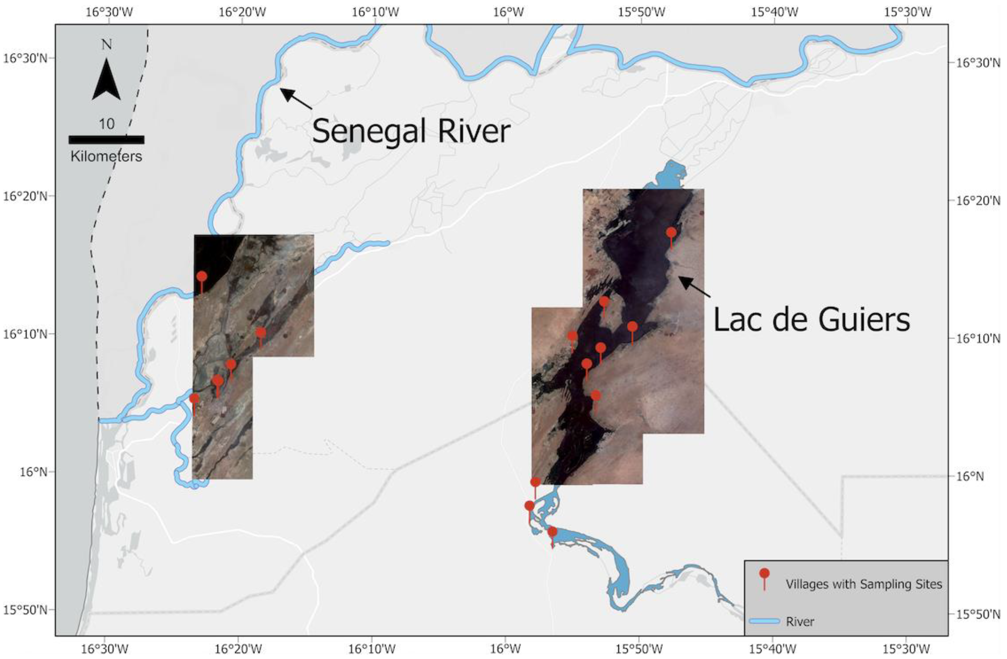
2.1. Study Area

The SRB, located in West Africa, covers 1.6% of the continent and spans four countries, with total basin size of about 337,000 km2. The Senegal River is a 1086-km-long river that forms the border between Senegal and Mauritania; it flows through large expanses of scarce Sahelian vegetation, with seasonally varying water levels [12]. We conducted field missions in the SRB seven times between 2016 and 2019, during which we visited 32 water access sites where human schistosomiasis transmission is known to occur, and collected various ecological and epidemiological data from 16 villages within the geographic coordinates 15.898277–16.317924°N and 15.767996–16.431078°W. Ten water access sites across six villages were located along the Senegal river and connected tributaries near the city of Saint-Louis, while the remaining 22 water access sites across 10 villages were located along the shores of Lac de Guiers, a 170 km2 freshwater lake located about 50 km east of the river sites and which overflows into the Senegal River (Figure 3).

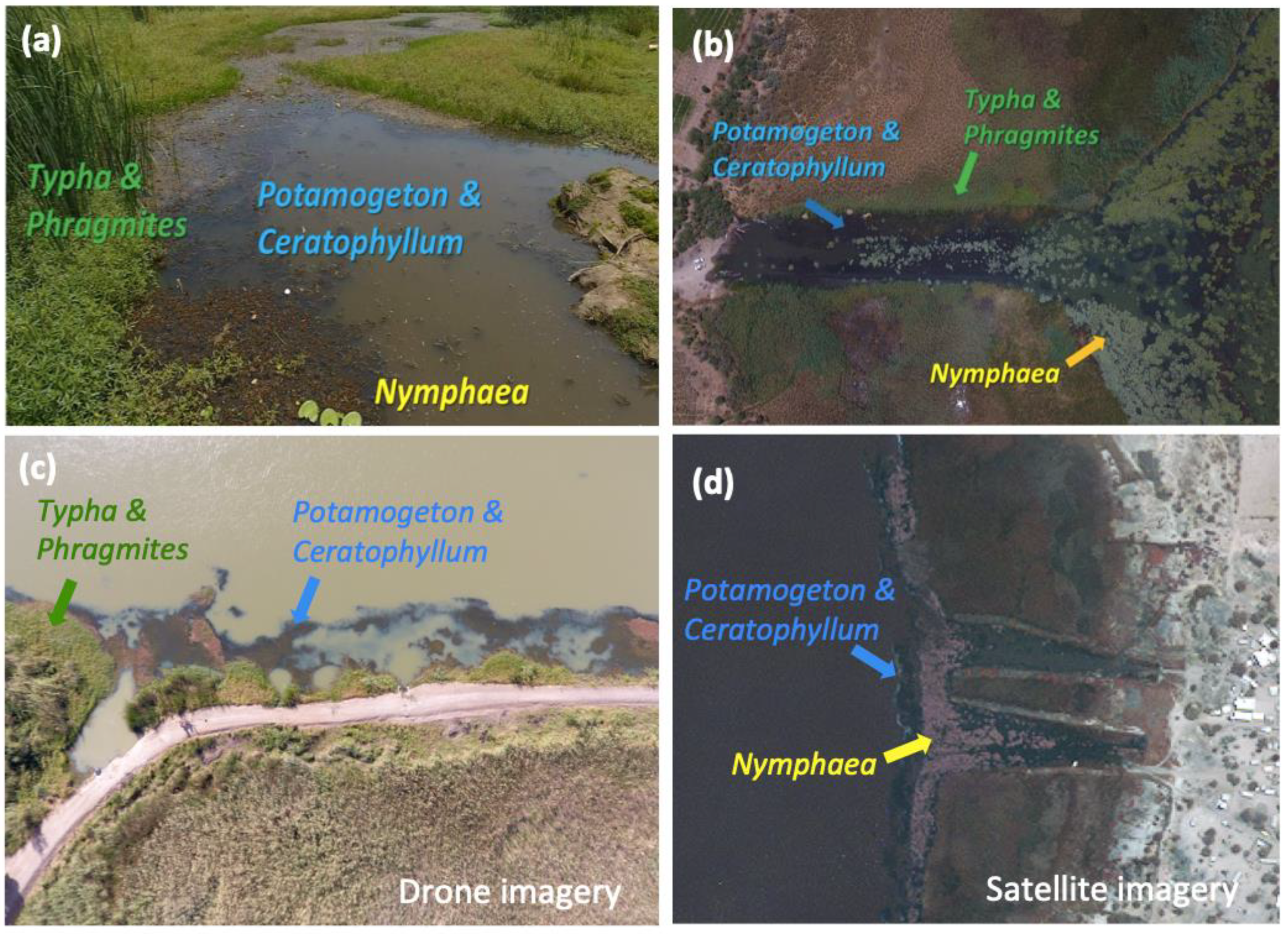
2.2. Remote Sensing Data and Vegetation Types
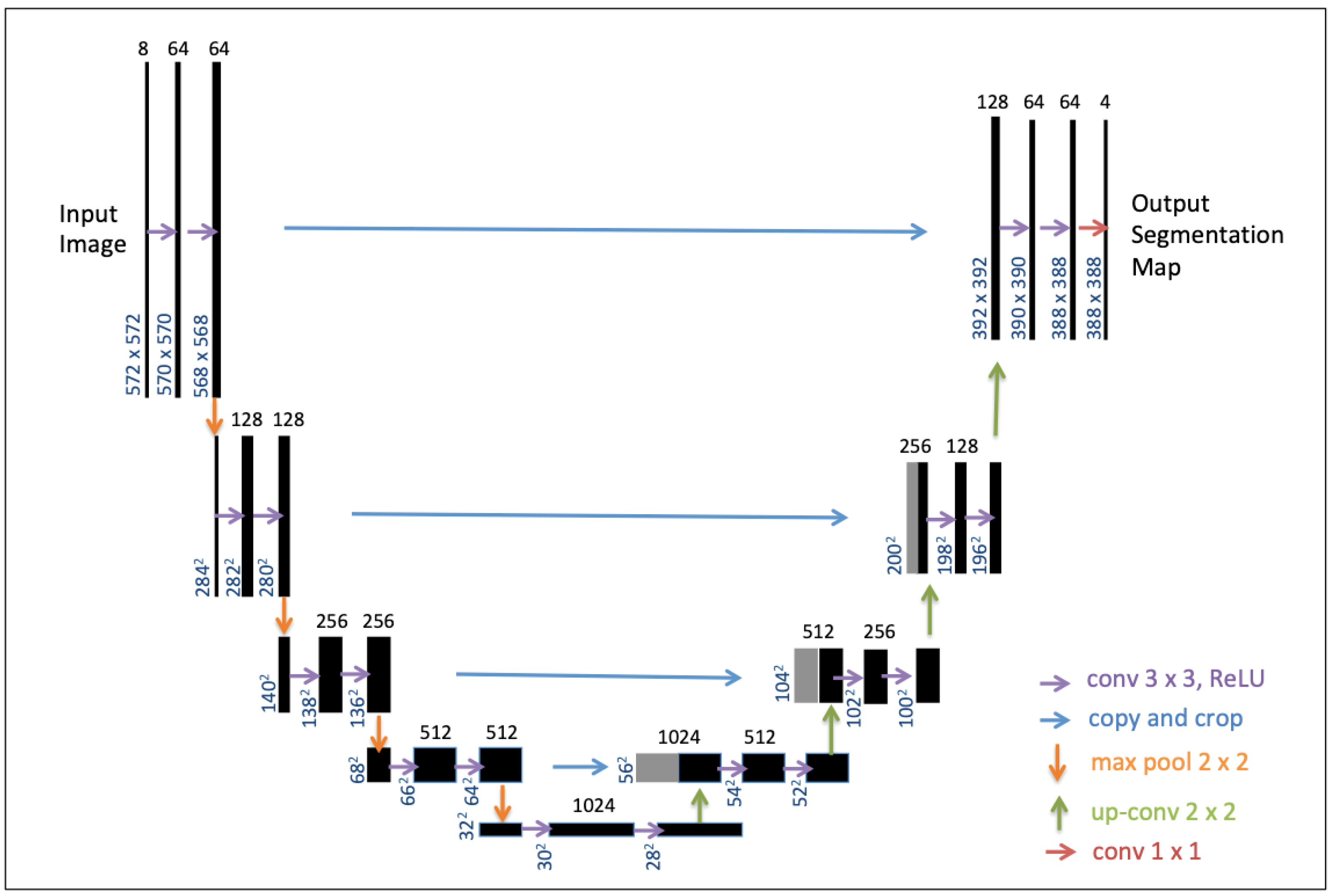
During field missions, we acquired more than 6000 high-resolution drone images using a DJI™ Phantom IV consumer drone equipped with the standard-issue 12.4-megapixel 1/2.3″-inch CMOS sensor. Each image consisted of RGB bands with average ground sample distance (GSD) of 2.31 cm/pixel and an average flight altitude of ~50 m above ground level, covering a total area of 15 km2. From drone images, several types of aquatic vegetation were identified visually: Potamogeton spp., Ceratophyllum spp., Typha spp., Phragmites spp., and Nymphaea spp. (Figure 2a,b). In most cases, Potamogeton spp. and Ceratophyllum spp. are associated with each other and are floating or lightly rooted and partially submerged in the water, while Typha spp. and Phragmites spp. form tall, dense stands of emergent vegetation along the edges of the water. Results from our previously published fieldwork [7] show that Bulinus spp. snails (obligate intermediate hosts for S. haematobium) are strongly associated with floating and lightly rooted aquatic vegetation, specifically the abundant, partially submerged plants Ceratophyllum spp. and Potamogeton spp. (Figure 2b), which appear as dark blue color patches on the water in RGB drone images. Drone imagery revealed sizable patches of suitable snail habitat distributed at great distances from the shore in areas inaccessible to traditional sampling methods. Results from our previous work show that measuring suitable snail habitat is a better predictor for disease risk and transmission than direct snail sampling methods [7]. Exploratory sampling from a boat also confirmed that schistosome-hosting snails were indeed present in offshore floating and submerged vegetation [7].
We used high-resolution drone imagery (Figure 2c) to validate the presence of various types of aquatic vegetation in coarser-resolution satellite images (Figure 2d). WorldView-2 multispectral satellite images were provided by the DigitalGlobe Foundation (now Maxar Technologies Inc., Westminster, CO, USA), including 36 mosaics covering a large area of our field sites in the SRB (Figure 3). These images were acquired between June and October 2016 and contain eight multispectral bands (Table 1) with a 2.0 m pixel spatial resolution. At this resolution, Ceratophyllum spp. and emergent vegetation are visible; however, it is not possible to distinguish Potamogeton spp. from Ceratophyllum spp., and Typha spp. from Phragmites spp. or Nymphaea spp. Therefore, we identify floating patches as the mixture of Potamogeton spp. and Ceratophyllum spp., and emergent patches as the mixture of Typha spp., Phragmites spp., and Nymphaea spp. (Figure 2c). About 90% of the imagery was cloudless. We selected 10 cloud-free mosaics covering our 32 water access points for deep learning training and validation. Images were gathered on 29 June 2016 (for river sites) and 4 July 2016 (for lake sites). Each selected mosaic has dimensions of 4096 × 4096 × 8 pixels. In order to generate our training set, we split each mosaic into 256 sub-images, each of 256 × 256 × 8 pixels.

2.3. Deep Learning

With recent advances in computation and the availability of large datasets, deep learning algorithms have been shown to be comparable with, and even exceed, human performance in image recognition tasks, including applications to diagnose human disease (e.g., [13] for ImageNet challenge, [14] for breast cancer histology images, and [15] for skin cancer images) as well as object detection [16,17], and semantic segmentation [9,18]. Convolutional neural networks (CNNs) learn key features directly from the training images by the optimization of the classification loss function and by interleaving convolutional and pooling layers, (i.e., spatially shrinking the feature maps layer by layer) [8,19]; in other words, CNNs exploit feature representations learned from raw image pixels and have minimal need for a priori knowledge and pre-defined statistical features [14,20]. Several studies have successfully implemented deep learning approaches and CNNs for various vegetation segmentation and classification tasks on satellite imagery and have achieved high accuracy [21,22,23].
A fully convolutional network (FCN) is a deep learning network for image segmentation [24]. Leveraging the advantages of convolutional computation in feature organization and extraction, an FCN establishes a multilayer convolution structure and de-convolution layers to realize pixel-by-pixel segmentation [9,25,26]. Segmentation models, such as FCNs, are effective because the multilayer structure of these models adeptly handles the detail features of images.
U-net—a specific type of FCN—has received a lot of interest for the segmentation of biomedical images using a reduced dataset [11] but has also proven to be very efficient for the pixel-wise classification of satellite images [22,27]. The U-Net architecture (Figure 4) consists of a contracting path to capture context and a symmetric expanding path that enables precise localization. Here, we adapted U-Net for semantic segmentation on aquatic vegetation using multispectral satellite imagery. For the design of our model, we followed the classical U-Net scheme that produced a state-of-the-art CNN encoder–decoder [11]. The workflow of our deep learning approach is presented in the next section.

2.4. Workflow and Model Implementation

The workflow of our deep learning approach of semantic segmentation on aquatic vegetation consisted of the following steps: (1) data preprocessing, (2) making label masks, (3) CNN model (U-Net architecture) training, (4) making predictions on new satellite imagery (i.e., inference) and producing example transmission risk maps for each image. Each step is described in the following sub-sections.

2.4.1. Data Preprocessing
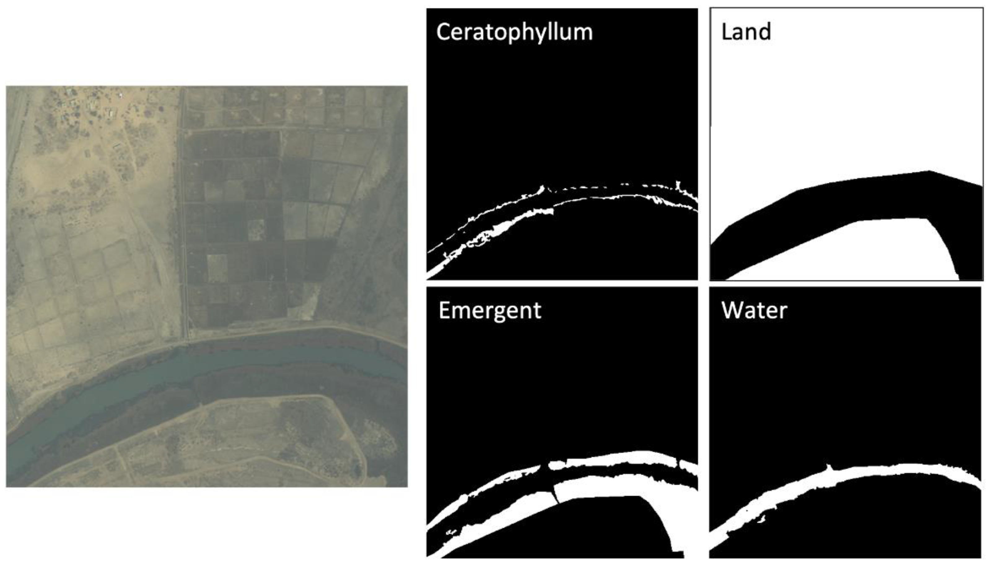
The calibration of multispectral satellite imagery was completed by DigitalGlobe before delivery, including correcting for radiometric and geometric sensor distortions [28]. Radiometric corrections include relative radiometric response between detectors, non-responsive detector fill, and conversion for absolute radiometry. Sensor corrections include corrections for internal detector geometry, optical distortion, scan distortion, line-rate variations, and misregistration of the multispectral bands. Each image had also been projected to UTM zone 28N using the WGS84 datum.
The eight bands of Worldview-2 imagery are Coastal, Blue, Green, Yellow, Red, Red Edge, NIR1, NIR2 (details in Table 1). Each pixel is geo-referenced and encoded as INT2U data type (hence, information is stored as digital numbers spanning 0–65,534). Before making label masks, we split each image mosaic into 16 sub-images of size 256 × 256 × 8, which was chosen as the input size for the U-Net model.

2.4.2. Label Masks

In this study, we defined four classes for the semantic segmentation task, namely floating, emergent, water, and land. As described above, the floating class encompassed most types of floating or lightly rooted and submerged aquatic vegetation, with Ceratophyllum spp. and Potamogeton spp. among others, and the emergent class identified mixed or uniform stands of mostly Typha spp. or Phragmites spp. vegetation, along with shorter emergent vegetation such as grasses and sedges at the water’s edges. The water class was simply areas devoid of either floating or emergent vegetation, with muddy bottom. The land class was non-water habitat and could be farmland, villages, terrestrial vegetation, or bare ground.
Technicians with extensive on-the-ground training and who were working directly with the identification and surveillance of aquatic vegetation at the sampling sites manually annotated 50 sub-images of WorldView-2 satellite imagery to create a binary mask for each class to use as training data. The manual annotation was completed via visual interpretation. The higher-resolution drone imagery was used to confirm the presence of each class on satellite data (Figure 2d) in the training set. Floating vegetation appears distinctly dark blue on drone and satellite imagery, which can help distinguish it from the green color of emergent vegetation. Therefore, for each image, four binary masks representing the four classes described above were produced. For example, a pixel of the floating mask has a value of 1 (white color) if it belongs to the floating class or a value of 0 (black color) if it belongs to any other class (Figure 5). There are no overlaps in the 256 × 256 labeled pixels for each class. Of the 50 × 4 masks, 80% were used as training/test set and 20% as hold-out validation/out-of-bag (OOB) set. Within the training set, 86% of the pixel area was water or land, 4% was floating vegetation, and 10% was emergent vegetation.

2.4.3. U-Net Training and Validation

Here, we followed the classical U-Net architecture (Figure 4), the CNN encoder–decoder [11], for the model design in the training. The network architecture consists of a contracting path (left side) and an expansive path (right side). The contracting path follows the typical architecture of a convolutional network, which is composed of Rectified Linear Units—i.e., the ReLU activation function—to avoid vanishing gradients and to improve the training speed [29], as well as of max-pooling layers. In total, the network has 23 convolutional layers. The final convolutional layer is used to map each 64-component feature vector to the 4 classes of our semantic segmentation task. Readers are referred to [11] for the details of the U-Net architecture.
We up-scaled the 256 × 256 × 8 preprocessed images to 572 × 572 × 8 as input layers in U-Net. The input images and their corresponding segmentation masks were used to train the network. Binary cross-entropy was selected as the loss function to evaluate the model weights of the CNN, and an accuracy metric was applied to measure how close the predicted mask was to the manually annotated masks pixel by pixel, namely:
Pixel accuracy = (TP + TN)/(TP + TN + FP + FN) (%)
where TP is true positive, TN is true negative, FP is false positive, and FN is false negative. The accuracy metric is defined by the number of pixels labeled correctly divided by the total number of pixels. During the training, the loss function was used to evaluate the performance of the U-Net by comparing the input data to the output values predicted. Stochastic gradient descent was implemented to iteratively adjust the weights, allowing the network to best approximate the training data output. At each iteration (i.e., epoch), a backpropagation algorithm estimated the partial derivatives of the loss function with respect to the incremental changes in all the weights to determine the gradient descent directions for the next iteration. The network weights were initialized randomly, and an adaptive learning rate gradient-descent back-propagation algorithm [29] was used to update model weights [8]. The model was trained with 80% of the training set and tested on the remaining images not used for training. Note that the test set was randomly selected for each epoch and was not used in the optimization or backpropagation algorithms. Instead, the loss function was evaluated over the hold-out validation data, and this served as an independent tuning metric of the performance of the U-Net.
Data augmentation and batch normalization were applied in the training. Data augmentation is essential to teach the network the desired invariance and robustness properties, when only a few training samples are available, especially for segmentation tasks [11]. In the model, we generated image transformations by randomly reversing and transposing first and second image dimensions. Dropout layers at the end of the contracting path were used for further implicit data augmentation. In practice, the random transformation allowed us to increase the size of the dataset without deteriorating its quality. Batch normalization is used for addressing internal covariate shift and is widely used in image segmentation [30]. In our model, we applied batch normalization after the convolution and before the activation. Data augmentation and batch normalization used here are expected to further improve the datasets and prediction performance.
We experimented with a set of hyperparameters for the learning algorithm, which included training epoch, batch size, and learning rate. We utilized these parameters to obtain a final accuracy after every run. We conducted a grid search hyperparameter tuning to obtain the optimal set of parameters whose values are used to control the learning process. The search space for the training epoch was {50, 100, 150}, and the batch size was {8, 16, 32, 64}. As for the learning rate, the first search space was {1 × 10⁻⁵, 1 × 10⁻⁴, 1 × 10⁻³, 1 × 10⁻²}, then we narrowed down the search to the best performing power group, for example, 1 × 10⁻⁵ to 9 × 10⁻⁵ with an increment of 1 × 10⁻⁵.
We implemented U-Net model and training in the Python development environment with the Keras package [31], which provides a high-level application programming interface to access Google’s deep learning framework, TensorFlow 2 [32]. Open Source code packages developed in this study can be accessed via the link provided in the Supplementary Materials Section.

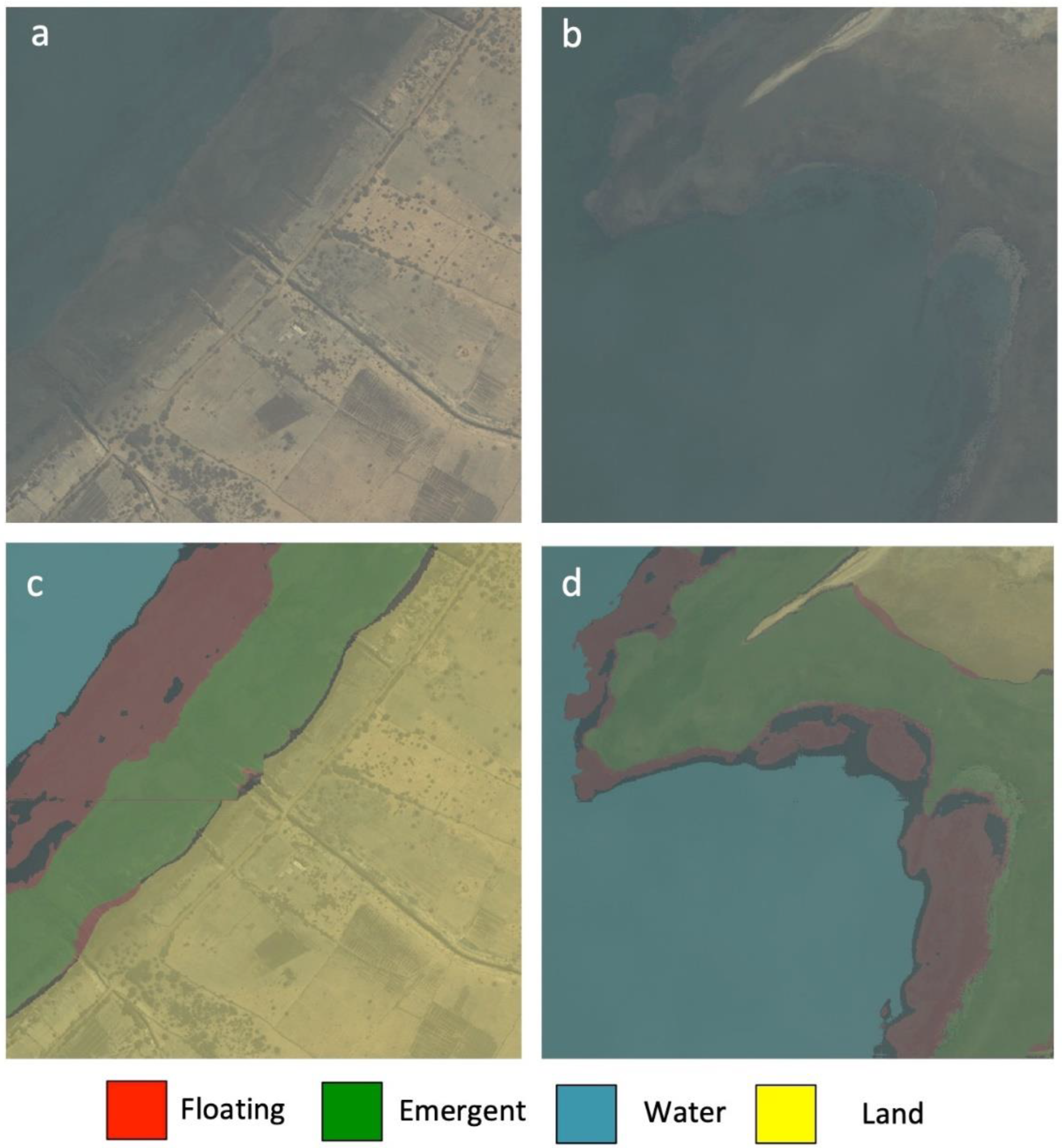
2.4.4. Inference and Heat Maps

After training the U-Net model and fine-tuning the network parameters in an iterative process, the best-performing model and corresponding weights were used to identify the aquatic vegetation on hold-out/OOB satellite data at the pixel level. With new input image feeds, our model outputs four layers of pixel-by-pixel segmentation, including floating vegetation, emergent vegetation, water, and land. Each output pixel prediction is accompanied by a probability of the object belonging to one of the four classes. For visualization purposes, we combined four layers of segmentation and color-coded each layer to form a single inference image. The inference image displaying the spatial distribution of the aquatic floating vegetation identified through field observations as the most suitable snail habitat can then be used for examining disease transmission risk [7].

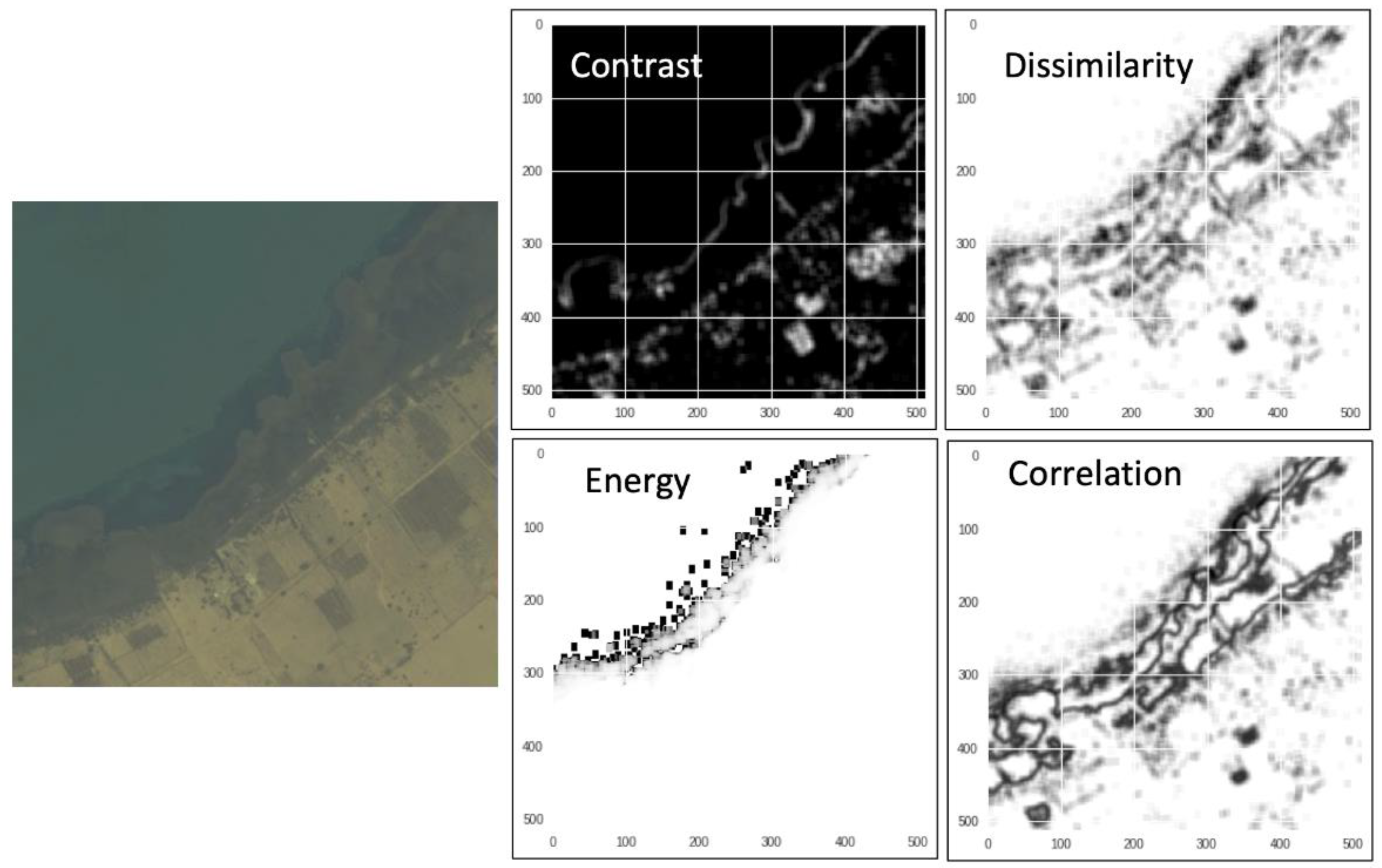
2.5. Benchmarking Deep Learning Performance against Random Forest

Additionally, we benchmarked U-Net formulations against a common modeling approach in the remote sensing community: random forest, a tree-based algorithm. Random forest analysis is a supervised ensemble classifier that generates unpruned classification trees to predict a response. Random forest implements bootstrapping samples of the data and randomized subsets of predictors [33]. Final predictions are ensembled across a forest of trees (n = 100) on the basis of an averaging of the probabilistic prediction of each classifier. No maxima were set for tree depth, number of leaf nodes, or number of features; we did this to favor prediction over interpretability.
Several studies [34,35,36,37,38] showed that random forest is a very efficient approach for land cover and vegetation classification from satellite imagery in environmental applications, especially when combined with a gray-level co-occurrence matrix (GLCM) textural analysis [39], a statistical approach to examine image texture based on the value and spatial relationships of pixels.
Here, we adapted the approach of [35] that combines GLCM with random forest for our segmentation task on aquatic vegetation in the SRB, and compared its prediction performance on the satellite data and on hold-out datasets not incorporated in the training set. With respect to the random forest approach, deep learning exploits feature representations learned exclusively from raw image pixels, without depending on additional statistical features, such as GLCM. However, for the purpose of comparison, we also trained a U-Net model with GLCM layers.
Six GLCM texture features, i.e., contrast, dissimilarity, homogeneity, energy, correlation, and angular second moment (Figure 6; see [40] for texture details), were calculated for each of the eight WorldView-2 multispectral bands by using Python scikit-image package version 0.15 [41]. The same input size (256 × 256 × 8) and the same batch of training and validation data of satellite imagery and corresponding masks were used in the random forest test, in comparison with the U-Net model.

3. Results

We evaluated the deep learning segmentation algorithm’s performance accuracy for the four classes (floating vegetation, emergent vegetation, water, and land) and experimented with multiple learning rates. We found the optimized batch size to be 8, training epoch to be 100, and learning rate to be 4 × 10⁻⁵, which resulted in a segmentation accuracy of 94.5% for the test set and 82.7% for the hold-out validation/OOB set, over all four classes. Color-coded inference maps were produced for visualization (Figure 7). Floating vegetation, which strongly predicts snail abundance and transmission risk in the SRB [7], represents the most important classification target for the problem at hand. When segmentation accuracy is computed only on the floating vegetation class, the U-Net model achieved an accuracy of 96% for the test set and 84% for the hold-out validation set.
Concerning the performance of the random forest model coupled with the six GLCM texture features, segmentation accuracy achieved 96.7% for the test set and 67.8% for the hold-out validation set, over all four classes, while the accuracy for the floating vegetation class was 97% for the test set and 68% for the validation set. When the U-Net model was trained by using the GLCM features, the segmentation accuracy was 96.5% for the test set and 83.1% for the hold-out validation set, over all four classes, while the accuracy for the floating vegetation class was 97.0% for the test set and 84.0% for the validation set. The results are summarized in Table 2.

4. Discussion

Our results demonstrate the ability of a deep learning segmentation approach to automatically identify the aquatic vegetation associated with snail species that act as intermediate hosts for transmission for schistosomiasis to humans in the lower SRB. Using high-resolution satellite imagery, our CNN-based model outperformed a commonly used random forest approach with regard to accuracy on validation data. This new framework applies a cutting-edge AI solution that has the capacity to provide a rapid, accurate, and cost-effective risk assessment for vegetation characteristics that have previously been elusive to quantify at large scales but have recently been shown to be correlated with urinary schistosomiasis transmission hotspots in the lower SRB [7]. This approach can be potentially applied and scaled to other areas subject to endemic schistosomiasis risk, especially where the ecology of local intermediate host snails is linked to the presence and extent of floating aquatic vegetation.
The deep learning workflow we presented here took considerable time for manual annotation (~200 human hours) on targeted vegetation and computing power to properly train the U-Net model. However, once trained and deployed, the deep learning model can analyze a satellite image and provide classification results extremely rapidly (in the scale of minutes). Our finding that the CNN (U-Net) model performed better than random forest approaches in the OOB dataset confirms previous findings that tree-based methods are less generalizable than deep learning segmentation methods [42]. In addition, adding GLCM texture layers to the U-Net model only marginally improved accuracy, which shows that deep learning does not heavily depend on the statistical features of the underlying image. Consequently, the CNN model does not require prior specification of GLCM layers by a domain expert, which makes the model less prone to bias due to researcher-specified inputs otherwise needed for conventional machine learning (e.g., random forest) approaches.
In general, the benefit of deep learning is to reduce the task of developing a new feature extractor for every problem as well as to avoid human biases when solving the problem. However, the limitation with deep learning is its interpretability. Mathematically it is possible to find out which nodes of a deep neural network were activated, but it is difficult to assess what these layers of neurons were doing collectively. On the other hand, conventional machine learning algorithms such as decision trees provide crisp rules on feature selections and decode for feature importance; therefore, it is easier to interpret the reasoning behind the model. In this study, we focus more on model prediction performance and accuracy than the interpretability, so deep learning is the preferred approach in this case.
The model evaluation metric selected here is pixel accuracy, which can sometimes provide misleading results when the class representation is very small within the image (<1%), as the measure will primarily be biased in reporting the model’s ability to identify negative cases (i.e., when the class is not present). This is not the concern for the imagery data used in this study, as the minor class achieved a very high segmentation performance around 97% accuracy. To further analyze the distributions of false positives of the predicted floating vegetation (see the black color pixels in the inference maps; Figure 7c,d), we found that most false positives were located along the edge of floating vegetation patches as well as the boundary with other vegetation, which indicates that more labeled pixels on the vegetation patches are required to improve the pixel accuracy of the model. However, the purpose of this study is to show the capability of generating rapid prediction and generalized mappings of the floating vegetation for the larger area instead of providing small details on how floating vegetation patches are distributed. The latter is more important in analyzing the seasonal changes in the floating vegetation and how it correlates with schistosomiasis transmission. This will be the focus of our follow-up studies.
In this study, the drone imagery was used to validate the presence and identity of aquatic vegetation on satellite imagery that was captured in a similar time period (less than a few months apart). For future studies, the drone imagery could have greater utilization in training deep learning models, e.g., for image super-resolution [43] as well as resolution enhancement [44] for satellite imagery in an adversarial training setting [45], as long as the satellite data is captured at the same time and place, ideally less than a few weeks apart, which would require precise planning and coordination of satellite image capture and drone operation activities. The opportunity to couple synchronous drone and satellite imagery becomes more and more feasible as more high-resolution satellites circle the Earth and create Earth observation data at a faster tempo. For example, the Planet satellite constellation now provides high-resolution satellite imagery with a global extent on a daily basis (https://www.planet.com, accessed on: 8 January 2022).
The segmentation algorithm and resultant aquatic vegetation inference maps presented here demonstrate proof of principle for the utility of a deep learning approach to enable production of aquatic vegetation maps with potential public health relevance for schistosomiasis transmission control. So far, the model has only been trained and validated over a relatively large spatial extent in the lower SRB, one of the most important hotspots for schistosomiasis transmission in the world, but there is strong potential to apply this model to larger spatial extents using remote sensing images from different river and lake systems to build a more generalized model. The next step in the development of this approach is to validate the predictive power of vegetation maps produced by this method for actual snail and human prevalence or incidence data. If indeed vegetation maps derived through the integration of high-definition satellite imagery with deep learning prove accurate in predicting snail presence or abundance and/or human infection risk across large scales, then this tool has the potential to provide unprecedented precision mapping of snail suitable habitat to efficiently target limited resources to control disease in the high-transmission areas. Future studies should thus focus on validating the ability of these vegetation inference maps to correctly predict human disease transmission in the SRB and other regions of Africa where there is endemic schistosomiasis transmission in a similar ecological context.

5. Conclusions

Recent analyses clearly show that area covered by suitable snail habitat (i.e., floating, non-emergent vegetation), percent cover by suitable snail habitat, and size of the water-contact area are more effective environmental proxies of human infection with schistosomiasis in the SRB than snail abundance estimates derived with traditional malacological field sampling [7]. In this work, we translated this ecological knowledge into practical tools for management through a deep learning model (U-Net) that is capable of automatically analyzing high-resolution satellite imagery to produce segmentation maps of aquatic vegetation associated with intermediate host snails, and potentially, with human schistosomiasis transmission. The performance of our deep learning model was more robust to generalization across different river and lake regions in the SRB than the more commonly used machine learning method of random forest and GLCM analysis. We show a proof of principle for how to create aquatic vegetation maps, including estimates of uncertainty, for identifying the possible intermediate host snail habitat hotspots in the SRB. We envision that these maps may allow local governments and health authorities to affordably obtain the most up-to-date spatial distribution of disease transmission at policy-relevant scales that were previously unobtainable, expanding capacity to address schistosomiasis environmental risks in this disease hotspot. This technology can be easily and affordably applied in other resource-poor settings where schistosomiasis is endemic and where identification of hotspots of transmission is desperately needed to target interventions. Our proof of principle shows that deep learning is a powerful tool that may help fill the capacity gap limiting our understanding of the environmental components of transmission for more affordable, efficient, and targeted control of neglected tropical diseases.

Supplementary Materials

Open-Source code packages developed in this study can be accessed via this link (https://github.com/deleo-lab/schisto-vegetation, accessed on: 8 January 2022).

Author Contributions

Z.Y.-C.L., K.T., L.L.L. and A.J.C. built, trained, and validated the U-Net model. A.J.C., I.J.J. and S.H.S. organized the dataset, while L.L.L. and A.J.C. labeled the image masks. A.J.C., I.J.J., S.H.S., G.A.D.L., C.L.W., N.J. and G.R. conducted the field work, while A.K.D. and L.L.L. assisted the field work. A.J.C., I.J.J., S.H.S., E.F.L. and G.A.D.L. conducted preliminary geospatial analysis. K.T. and J.B. further improved the U-Net model and training process. G.A.D.L. conceived the original idea and supervised the project in all perspectives. All the other authors (M.B., C.M.W., R.C., L.M. (Lorenzo Mari), M.G., L.T., J.R.R., L.M. (Lisa Mandle) and G.D.) participated in the project and contributed to finalize the paper. All authors have read and agreed to the published version of the manuscript.

Funding

This work was supported by a grant from the Bill and Melinda Gates Foundation (OPP1114050), an Environmental Ventures Program grant from Stanford University Woods Institute for the Environment, a SEED grant from the Freeman Spogli Institute at Stanford University, a Human Centered Artificial Intelligence (HAI) grant and a Woods Institute for the Environment EVP grant from Stanford University, and from the National Science Foundation (DEB-2011179 and grants ICER-2024383). CLW was supported by the Michigan Society of Fellows at the University of Michigan. JRR was supported by NSF DEB-2109293, DEB-2017785 and a grant for the Indiana Clinical and Translational Sciences Institute.

Institutional Review Board Statement

Not applicable.

Informed Consent Statement

Not applicable.

Data Availability Statement

Open-Source dataset developed in this study can be accessed via this link (https://github.com/deleo-lab/schisto-vegetation, accessed on: 8 January 2022).

Acknowledgments

We thank Paroma Varma, Tim White, Richard Grewelle, Paul Van Eck, and Ton Ngo for their suggestions and comments for this project. We also thank DigitalGlobe Foundation for the WorldView-2 satellite imagery used in this study. The authors are thankful also to Mouhamed Moustapha Fall, AIMS-Senegal, for his support to the present work.

Conflicts of Interest

The authors declare no conflict of interest.

References

  1. Steinmann, P.; Keiser, J.; Bos, R.; Tanner, M.; Utzinger, J. Schistosomiasis and water resources development: Systematic review, meta-analysis, and estimates of people at risk. Lancet Infect. Dis. 2006, 6, 411–425. [Google Scholar] [CrossRef]
  2. Hotez, P.J.; Kamath, A. Neglected tropical diseases in sub-Saharan Africa: Review of their prevalence, distribution, and disease burden. PLoS Negl. Trop. Dis. 2009, 3, e412. [Google Scholar] [CrossRef] [PubMed] [Green Version]
  3. Danso-Appiah, T. Schistosomiasis. In Neglected Tropical Diseases—Sub-Saharan Africa; Gyapong, J., Boatin, B., Eds.; Springer: Cham, Switzerland, 2016. [Google Scholar]
  4. Remais, J.V.; Eisenberg, J.N. Balance between clinical and environmental responses to infectious diseases. Lancet 2012, 379, 1457–1459. [Google Scholar] [CrossRef] [Green Version]
  5. Sokolow, S.H.; Wood, C.L.; Jones, I.J.; Swartz, S.J.; Lopez, M.; Hsieh, M.H.; Lafferty, K.D.; Kuris, A.M.; Rickards, C.; De Leo, G.A. Global assessment of schistosomiasis control over the past century shows targeting the snail intermediate host works best. PLoS Negl. Trop. Dis. 2016, 10, e0004794. [Google Scholar] [CrossRef]
  6. Sokolow, S.H.; Wood, C.L.; Jones, I.J.; Lafferty, K.D.; Kuris, A.M.; Hsieh, M.H.; De Leo, G.A. To reduce the global burden of human schistosomiasis, use ‘old fashioned ‘snail control. Trends Parasitol. 2018, 34, 23–40. [Google Scholar] [CrossRef] [PubMed]
  7. Wood, C.L.; Sokolow, S.H.; Jones, I.J.; Chamberlin, A.J.; Lafferty, K.D.; Juris, A.M.; Jocques, M.; Hopkins, S.; Adams, G.; Schneider, M.; et al. Precision mapping of snail habitat provides a powerful indicator of human schistosomiasis transmission. Proc. Natl. Acad. Sci. USA 2019, 116, 23182–23191. [Google Scholar] [CrossRef] [Green Version]
  8. LeCun, Y.; Bengio, Y.; Hinton, G. Deep learning. Nature 2015, 521, 436. [Google Scholar] [CrossRef] [PubMed]
  9. Long, J.; Shelhamer, E.; Darrell, T. Fully convolutional networks for semantic segmentation. In Proceedings of the IEEE Conference on Computer Vision and Pattern Recognition, Boston, MA, USA, 6–12 June 2015; pp. 3431–3440. [Google Scholar]
  10. Jones, I.J.; Sokolow, S.H.; Chamberlin, A.J.; Lund, A.J.; Jouanard, N.; Bandagny, L.; Ndione, R.; Senghor, S.; Schacht, A.M.; Riveau, G.; et al. Schistosome infection in Senegal is associated with different spatial extents of risk and ecological drivers for Schistosoma haematobium and S. mansoni. PLoS Negl. Trop. Dis. 2021, 15, e0009712. [Google Scholar] [CrossRef] [PubMed]
  11. Ronneberger, O.; Fischer, P.; Brox, T. U-net: Convolutional networks for biomedical image segmentation. In International Conference on Medical Image Computing and Computer-Assisted Intervention; Springer: Cham, Switzerland, 2015; pp. 234–241. [Google Scholar]
  12. Sow, S.; De Vlas, S.J.; Engels, D.; Gryseels, B. Water-related disease patterns before and after the construction of the Diama dam in northern Senegal. Ann. Trop. Med. Parasitol. 2002, 96, 575–586. [Google Scholar] [CrossRef] [PubMed]
  13. Russakovsky, O.; Deng, J.; Su, H.; Krause, J.; Satheesh, S.; Ma, S.; Huang, Z.; Karpathy, A.; Khosla, A.; Bernstein, M.; et al. Imagenet large scale visual recognition challenge. Int. J. Comput. Vis. 2015, 115, 211–252. [Google Scholar] [CrossRef] [Green Version]
  14. Araújo, T.; Aresta, G.; Castro, E.; Rouco, J.; Aguiar, P.; Eloy, C.; Polónia, A.; Campilho, A. Classification of breast cancer histology images using convolutional neural networks. PLoS ONE 2017, 12, e0177544. [Google Scholar] [CrossRef] [PubMed]
  15. Esteva, A.; Kuprel, B.; Novoa, R.A.; Ko, J.; Swetter, S.M.; Blau, H.M.; Thrun, S. Dermatologist-level classification of skin cancer with deep neural networks. Nature 2017, 542, 115–118. [Google Scholar] [CrossRef] [PubMed]
  16. Girshick, R.; Donahue, J.; Darrell, T.; Malik, J. Region-based convolutional networks for accurate object detection and segmentation. IEEE Trans. Pattern Anal. Mach. Intell. 2015, 38, 142–158. [Google Scholar] [CrossRef] [PubMed]
  17. Redmon, J.; Divvala, S.; Girshick, R.; Farhadi, A. You only look once: Unified, real-time object detection. In Proceedings of the IEEE Conference on Computer Vision and Pattern Recognition, Honolulu, HI, USA, 21–26 July 2016; pp. 779–788. [Google Scholar]
  18. Noh, H.; Hong, S.; Han, B. Learning deconvolution network for semantic segmentation. In Proceedings of the IEEE International Conference on Computer Vision, Boston, MA, USA, 6–12 June 2015; pp. 1520–1528. [Google Scholar]
  19. LeCun, Y.; Bengio, Y. Convolutional networks for images, speech, and time series. Handb. Brain Theory Neural Netw. 1995, 3361, 1995. [Google Scholar]
  20. Spanhol, F.A.; Oliveira, L.S.; Petitjean, C.; Heutte, L. Breast cancer histopathological image classification using convolutional neural networks. In Proceedings of the International Joint Conference on Neural Networks (IJCNN), Vancouver, BC, Canada, 24–29 July 2016; pp. 2560–2567. [Google Scholar]
  21. Langford, Z.L.; Kumar, J.; Hoffman, F.M. Convolutional neural network approach for mapping arctic vegetation using multi-sensor remote sensing fusion. In Proceedings of the IEEE International Conference on Data Mining Workshops (ICDMW), New Orleans, LA, USA, 18–21 November 2017; pp. 322–331. [Google Scholar]
  22. Rakhlin, A.; Davydow, A.; Nikolenko, S.I. Land Cover Classification From Satellite Imagery With U-Net and Lovasz-Softmax Loss. In Proceedings of the CVPR Workshops, Salt Lake City, UT, USA, 18–22 June 2018; pp. 262–266. [Google Scholar]
  23. Zhang, P.; Ke, Y.; Zhang, Z.; Wang, M.; Li, P.; Zhang, S. Urban land use and land cover classification using novel deep learning models based on high spatial resolution satellite imagery. Sensors 2018, 18, 3717. [Google Scholar] [CrossRef] [PubMed] [Green Version]
  24. Chen, L.C.; Papandreou, G.; Kokkinos, I.; Murphy, K.; Yuille, A.L. Semantic image segmentation with deep convolutional nets and fully connected crfs. arXiv 2014, arXiv:1412.7062. [Google Scholar]
  25. Fu, G.; Liu, C.; Zhou, R.; Sun, T.; Zhang, Q. Classification for high resolution remote sensing imagery using a fully convolutional network. Remote Sens. 2017, 9, 498. [Google Scholar] [CrossRef] [Green Version]
  26. Dolz, J.; Desrosiers, C.; Ayed, I.B. 3D fully convolutional networks for subcortical segmentation in MRI: A large-scale study. NeuroImage 2018, 170, 456–470. [Google Scholar] [CrossRef] [Green Version]
  27. Iglovikov, V.; Mushinskiy, S.; Osin, V. Satellite imagery feature detection using deep convolutional neural network: A kaggle competition. arXiv 2017, arXiv:1706.06169. [Google Scholar]
  28. Cheng, P.; Chaapel, C. Pan-sharpening and geometric correction: Worldview-2 satellite. GeoInformatics 2010, 13, 30. [Google Scholar]
  29. Nair, V.; Hinton, G.E. Rectified linear units improve restricted boltzmann machines. In Proceedings of the 27th International Conference on Machine Learning (ICML-10), Haifa, Israel, 21–24 June 2010; pp. 807–814. [Google Scholar]
  30. Zhou, X.Y.; Yang, G.Z. Normalization in training U-Net for 2-D biomedical semantic segmentation. IEEE Robot. Autom. Lett. 2009, 4, 1792–1799. [Google Scholar] [CrossRef] [Green Version]
  31. Chollet, F. Keras. GitHub. 2015. Available online: https://github.com/fchollet/keras (accessed on 8 January 2022).
  32. Abadi, M.; Barham, P.; Chen, J.; Chen, Z.; Davis, A.; Dean, J.; Devin, M.; Ghemawat, S.; Irving, G.; Isard, M.; et al. Tensorflow: A system for large-scale machine learning. In Proceedings of the 12th USENIX Symposium on Operating Systems Design and Implementation (OSDI 16), Savannah, GA, USA, 2–4 November 2016; pp. 265–283. [Google Scholar]
  33. Breiman, L. Random forests. Mach. Learn. 2001, 45, 5–32. [Google Scholar] [CrossRef] [Green Version]
  34. Bricher, P.K.; Lucieer, A.; Shaw, J.; Terauds, A.; Bergstrom, D.M. Mapping sub-Antarctic cushion plants using random forests to combine very high resolution satellite imagery and terrain modelling. PLoS ONE 2013, 8, e72093. [Google Scholar] [CrossRef] [PubMed]
  35. Burnett, M.W.; White, T.D.; McCauley, D.J.; De Leo, G.A.; Micheli, F. Quantifying coconut palm extent on Pacific islands using spectral and textural analysis of very high resolution imagery. Int. J. Remote Sens. 2019, 40, 7329–7355. [Google Scholar] [CrossRef]
  36. Kaszta, Ż.; Van De Kerchove, R.; Ramoelo, A.; Cho, M.; Madonsela, S.; Mathieu, R.; Wolff, E. Seasonal separation of African savanna components using worldview-2 imagery: A comparison of pixel-and object-based approaches and selected classification algorithms. Remote Sens. 2016, 8, 763. [Google Scholar] [CrossRef] [Green Version]
  37. Murray, H.; Lucieer, A.; Williams, R. Texture-based classification of sub-Antarctic vegetation communities on Heard Island. Int. J. Appl. Earth Obs. Geoinf. 2010, 12, 138–149. [Google Scholar] [CrossRef]
  38. Wang, T.; Zhang, H.; Lin, H.; Fang, C. Textural–spectral feature-based species classification of mangroves in Mai Po Nature Reserve from Worldview-3 imagery. Remote Sens. 2016, 8, 24. [Google Scholar] [CrossRef] [Green Version]
  39. Haralick, R.M.; Shanmugam, K. Textural features for image classification. IEEE Trans. Syst. Man Cybern. 1973, 6, 610–621. [Google Scholar] [CrossRef] [Green Version]
  40. Hall-Beyer, M. Practical guidelines for choosing GLCM textures to use in landscape classification tasks over a range of moderate spatial scales. Int. J. Remote Sens. 2017, 38, 1312–1338. [Google Scholar] [CrossRef]
  41. Van der Walt, S.; Schönberger, J.L.; Nunez-Iglesias, J.; Boulogne, F.; Warner, J.D.; Yager, N.; Gouillart, E.; Yu, T. Scikit-image: Image processing in Python. PeerJ 2014, 2, e453. [Google Scholar] [CrossRef] [PubMed]
  42. Tang, C.; Garreau, D.; von Luxburg, U. When do random forests fail? Adv. Neural Inf. Process. Syst. 2018, 31, 2983–2993. [Google Scholar]
  43. Yang, W.; Zhang, X.; Tian, Y.; Wang, W.; Xue, J.H.; Liao, Q. Deep learning for single image super-resolution: A brief review. IEEE Trans. Multimed. 2019, 21, 3106–3121. [Google Scholar] [CrossRef] [Green Version]
  44. Sajjadi, M.S.; Scholkopf, B.; Hirsch, M. Enhancenet: Single image super-resolution through automated texture synthesis. In Proceedings of the IEEE International Conference on Computer Vision, Venice, Italy, 22–29 October 2017; pp. 4491–4500. [Google Scholar]
  45. Goodfellow, I.J.; Pouget-Abadie, J.; Mirza, M.; Xu, B.; Warde-Farley, D.; Ozair, S.; Courville, A.; Bengio, Y. Generative adversarial networks. arXiv 2014, arXiv:1406.2661. [Google Scholar] [CrossRef]
Figure 1. (a) The life cycle of Schistosoma spp. parasites. The adult worms live and reproduce sexually within the human host, releasing eggs into the environment that hatch and seek an intermediate freshwater snail host, where the larval stages of the worms develop via asexual reproduction. Cercariae are released from snails and seek human hosts, completing the life cycle. (b) Sampling aquatic environments for infected snails is physically demanding, time-intensive, and limited to accessible areas. Snails are found by sifting through thick vegetation, and later processed in the laboratory for parasitological data.
Remotesensing 14 01345 g001
Figure 2. (a) Typical vegetation types found at water access points in the SRB, as seen from the shoreline (b,c) through drone imagery and (d) satellite imagery (WorldView-2). Specific vegetation types are a key indicator of snail presence and abundance and extend far beyond the area safely sampled by trained technicians, thus limiting accurate estimates for human disease risk.
Remotesensing 14 01345 g002
Figure 3. A mosaic of Maxar Technologies Inc., Westminster, CO, USA (formerly DigitalGlobe) WorldView-2 imagery of our study area, the SRB. Red markers indicate the locations of our 32 sampling sites.
Remotesensing 14 01345 g003
Figure 4. U-net architecture reproduced from [11]. The black boxes correspond to a multi-channel feature map. The number of channels is denoted on top of the box. The x-y-size is provided at the lower left edge of the box. Gray boxes represent copied feature maps. The colored arrows denote the separated operations. The final segmentation layer outputs 4 classes of labels for this study. Details refer to [11].
Remotesensing 14 01345 g004
Figure 5. Example of label masks for a satellite image. The four classes are floating, emergent, water, and land’. Pixels are assigned a value of 1 (white color) if they belong to the assigned class, and a value of 0 (black color) otherwise.
Remotesensing 14 01345 g005
Figure 6. Examples of GLCM texture features: contrast, dissimilarity, energy, and correlation, which are calculated from the raw pixel values of the 8-band multispectral WorldView-2 imagery.
Remotesensing 14 01345 g006
Figure 7. Comparison between satellite images and the corresponding inference maps. (a,b) WorldView-2 satellite imagery, (c,d) inference map (red: floating; green: emergent; blue: water; yellow: land) produced by the trained U-Net model. The black colored pixels on the inference map refer to the false positive values of floating vegetation.
Remotesensing 14 01345 g007
Table 1. WorldView-2’s eight multispectral bands.
Scheme 397Wavelength (nm)
Coastal397–454
Blue445–517
Green507–586
Yellow580–629
Red626–696
Red Edge698–749
Near-IR 1765–899
Near-IR 2857–1039
Table 2. Summary of model results on test set and hold-out validation set.
Model GLCM FeaturesTest Set Accuracy—4 ClassesHold-Out Validation Set Accuracy—4 ClassesTest Set Accuracy—Floating VegetationHold-Out Validation Set Accuracy—Floating Vegetation
Random forest Added96.7%67.8%97.0%68.0%
CNN-based (U-Net) Not94.5%82.7%96.0%84.0%
Added96.5%83.1%97.0%84.0%
Publisher’s Note: MDPI stays neutral with regard to jurisdictional claims in published maps and institutional affiliations.

