Article

A Neural Network Method for Retrieving Sea Surface Wind Speed for C-Band SAR

1
College of Computer and Information Engineering, Xiamen University of Technology, Xiamen 361024, China
2
Key Laboratory of Spatial Data Mining and Information Sharing of Ministry of Education, National Engineering Research Centre of Geo-Spatial Information Technology, Fuzhou University, Fuzhou 350002, China
3
College of Harbour and Coastal Engineering, Jimei University, Xiamen 361021, China
4
Nansen Environmental and Remote Sensing Center and Geophysical Institute, University of Bergen, N-5006 Bergen, Norway
5
Center for Remote Sensing, College of Earth, Ocean and Environment, University of Delaware, Newark, DE 19716, USA
6
Fujian Engineering Research Center for Ocean Remote Sensing Big Data, Xiamen University, Xiamen 361005, China
7
School of Marine Sciences, Sun Yat-sen University, Guangzhou 510080, China
8
Southern Marine Science and Engineering Guangdong Laboratory (Zhuhai), Zhuhai 519000, China
*
Author to whom correspondence should be addressed.
Submission received: 12 February 2022 / Revised: 3 May 2022 / Accepted: 5 May 2022 / Published: 8 May 2022

Abstract

:
Based on the Ocean Projection and Extension neural Network (OPEN) method, a novel approach is proposed to retrieve sea surface wind speed for C-band synthetic aperture radar (SAR). In order to prove the methodology with a robust dataset, five-year normalized radar cross section (NRCS) measurements from the advanced scatterometer (ASCAT), a well-known side-looking radar sensor, are used to train the model. In situ wind data from direct buoy observations, instead of reanalysis wind data or model results, are used as the ground truth in the OPEN model. The model is applied to retrieve sea surface winds from two independent data sets, ASCAT and Sentinel-1 SAR data, and has been well-validated using buoy measurements from the National Oceanic and Atmospheric Administration (NOAA) and China Meteorological Administration (CMA), and the ASCAT coastal wind product. The comparison between the OPEN model and four C-band model (CMOD) versions (CMOD4, CMOD-IFR2, CMOD5.N, and CMOD7) further indicates the good performance of the proposed model for C-band SAR sensors. It is anticipated that the use of high-resolution SAR data together with the new wind speed retrieval method can provide continuous and accurate ocean wind products in the future.

1. Introduction

In the ocean, the surface wind field is one of the most important parameters for a range of activities, both for scientific and application purposes [1]. It is widely used to study sea surface waves [2], wind-driven currents [3], ocean circulation [4], offshore fronts, marine biogeochemistry [5], energy, and material exchange between the ocean and atmosphere for research in oceanography and meteorology. It is also an indispensable factor to provide help for the safety and security of human activities, i.e., oceanographic survey, fisheries, oil spill monitoring, maritime navigation, and other coastal and marine operations.
Traditional means to obtain the ocean surface wind field include irregular ship reports and fixed meteorological stations and buoys [6]. However, the acquisition cost and weather limitation hinder the continuity and availability of wind data by means of cruise observations. Measurements from offshore buoys and meteorological stations are spatially sparse and cannot fully meet the needs of scientific and applied goals in coastal and marine activities [7]. To meet the requirements for wind observations, satellite-borne microwave radar, scatterometers, radiometers, and synthetic aperture radar (SAR), can be used to observe the sea surface wind field in a large spatial scale under all-time and all-weather conditions [8]. Among these sensors, SAR is a unique tool to allow for high-resolution (finer than 1 km) observations of the near-surface wind field, which is more practical in coastal regions [9], with low costs and short revisiting time [10]. The ongoing spaceborne SAR missions have already proven their success on such applications, including Radarsat-2 [11], Sentinel-1 [12], and Gaofen-3 [13]. As small satellites and constellations develop rapidly, the outlook on CubeSat and small satellite SAR-based missions is also economically promising for obtaining ocean winds [14].
Radar sensors are very sensitive to the ocean surface roughness (or normalized radar cross section, denoted by NRCS or σ0) [15,16]. The σ0 measured by SAR systems can be used to provide sea surface wind speed at a 10 m height (U10) using empirical geophysical model functions (GMFs). At present, the C-band model (CMOD) functions, e.g., CMOD4 [17], CMOD-IFR2 [18], CMOD5 [19], and CMOD5.N [20], developed based on NRCS measurements in VV (vertical-vertical) polarization from scatterometers are still commonly used GMFs to retrieve coastal winds for SAR sensors [8]. Similar C-band GMFs have also been developed based on SAR measured backscatter data [21,22]. These C-band GMFs are a function of the sea surface roughness, incidence angle, polarization, and relative azimuth between radar look angle and wind directions. Since the physical relationship between a wind vector and its radar signal is not easy to understand [23], parameters in GMFs should be regressed using different sources of reference winds, such as those from numerical models [17] and buoy data [18,24]. To date, the CMOD functions have been updated to the latest CMOD7 for advanced scatterometer (ASCAT) [25], and the European Space Agency (ESA) is still continuously improving their performance on 10 m-height stress-equivalent winds [26], quality assessment [27], and extreme winds [28].
GMFs are nonlinear transfer functions leading to a complicated inverse problem. Such nonlinear regression problems can be easily solved using the neural network (NN) technique [29,30]. Machine learning methods have also demonstrated their great potential in some ocean remote sensing areas [31]. Some C-band GMFs based on machine learning methods have been proposed to compute wind vectors. Thiria et al. [32] first proposed a quasi-linear multilayer perceptrons (MLP) method to compute wind speeds based on the σ0 triplet of simulated ERS-1 scatterometer data. The accuracy of the retrieved wind vector was then improved by a mixture density network (MDN) with circular normal kernel densities for C-band observations [33,34,35]. As for the SAR retrieval of sea surface wind speed, Horstmann et al. [36] proposed a straightforward method to retrieve wind speeds for uncalibrated SAR data in wave mode from the European Remote Sensing (ERS) satellites ERS-2. The NN-based model was trained using 27 days of ERS-2 SAR data and collocated wind data from the European Centre for Medium-Range Weather Forecast (ECMWF) model data. Shao et al. [37] built a collocated dataset between the ECMWF winds and Gaofen-3 SAR data, and then proposed a wind retrieval model using four NN methods, gradient boosting decision tree, back-propagation (BP), K nearest neighbors, and random forest. Their research confirmed the applicability of NN method for quad-polarization SAR data compared with ASCAT winds. Considering that HH-polarized SAR data have been extensively acquired over the Arctic region for polar monitoring, Qin et al. [38] utilized a GMF-guided NN to retrieve winds using ASCAT winds and Sentinel-1 SAR images in EW mode. The BP NN-based model was further improved with a larger amount of collocated ASCAT and Sentinel-1 data [39].
In previous NN-based studies, most of them used reference winds from numerical models, reanalysis data, or GMFs to train the network. Studies are possible using direct in situ data from long-term buoy observations to train the model. In addition, in our previous work, we found a good generalization capability to combine an MLPs model with a Bayesian Regularization scheme in regression problems [40,41]. This approach is termed the Ocean Projection and Extension neural Network (OPEN) method [41] and has shown its potential and merits in constructing global heat content [42]. Yet, this method has never been applied in the retrieval of remote sensing wind speed.
The purpose of this study is to propose a new wind speed retrieval method for single-antenna SAR sensors, which may help to provide accurate and high-resolution coastal and ocean wind speeds both for scientific and applied purposes. Since co-polarization NRCSs are still the most reliable and easily collected data from ongoing SAR, especially for the freely available Sentinel-1 with relatively high residual noise in cross-polarization data [43,44] and small satellites such as Hisea-1 with only co-polarization measurements [14], the OPEN method is examined to retrieve sea surface wind speeds for VV polarization C-band SAR in this study. To prove the methodology with a robust dataset, a long record of NRCS measurements from ASCAT, which is a well-known C-band radar sensor [25], are used to train the model. In situ wind observations exclusively from buoys are collocated with ASCAT data from 2013 to 2017 and used as the label data for our network. Descriptions of the datasets and methods are presented in Section 2. Section 3 validates and compares the model results using ASCAT, Sentinel-1 SAR, and buoy data. Discussions and conclusions are provided in Section 4 and Section 5.

2. Data and Methods

2.1. Data Sets

2.1.1. ASCAT Data

ASCAT is one of the instruments aboard the Meteorological Operational (MetOp) satellites with an altitude of 817 km, which are operated by the European Organization for the Exploitation of Meteorological Satellites (EUMETSAT). It is a C-band real aperture radar with six beam antennas, providing three σ0 measurements in VV polarization, both to the left and right side along the satellite track. The Royal Netherlands Meteorological Institute (KNMI) (https://scatterometer.knmi.nl/home/ accessed on 1 February 2022) is now responsible for the operational deployment of the ASCAT wind products. Currently, ASCAT can provide wind products with spatial resolutions of 12.5 km and 25 km. Since C-band series scatterometers have been used operationally to produce sea surface wind vectors on a global scale in the past decades based on NRCS measurements [25], it can be considered a robust sensor to provide reliable data for training and validating a GMF for C-band SAR.
In this study, the coastal wind products with a resolution of 12.5 km onboard the MetOp-A and MetOp-B satellites, launched in October 2006 and September 2012, are used to train and validate the model. The individual NRCS observations for the coastal products have been processed by a boxcar spatial filtering by the KNMI to provide more wind vectors close to the coast [45], which is useful for the application of the proposed model in the coastal area. Since SAR can only provide NRCSs from its single antenna, observations from other two poses are abandoned except for the data from the middle beam. Measurements including middle-beam incidence angle, azimuth, and σ0 in decibels (dB) for years from 2013 to 2017 are extracted from the coastal products. These data are in BUFR format and are further handled by the BUFR Reader program developed by KNMI to collocate with the buoy data. Note that the ASCAT NRCS measurements have not been processed by an ocean calibration to keep consistent with SAR data. The wind speeds from ASCAT 12.5 km coastal wind product are also used to validate the derived wind results by the proposed NN model.

2.1.2. Sentinel-1 SAR Data

The Sentinel-1 mission designed by ESA can provide freely available C-band SAR data with side-looking radars. The SAR mission consists of two satellites, Sentinel-1A and Sentinel-1B, which were launched in April 2014 and April 2016. It allows for the observation of ocean surface roughness with a very high spatial resolution (less than 100 m). The Level-1 Ground Range Detected (GRD) SAR images in the VV band with interferometric wide (IW) swath mode are collected to validate the proposed model. These SAR data are processed using the Sentinel Application Platform (SNAP). The processing steps include removal of low-intensity GRD border noise, thermal noise removal, radiometric calibration, and refined lee filtering [46]. The pixel spacing of the SAR imagery is averaged to 1 km × 1 km to suppress the speckle noise. Given such a cell size, the mean radiometric resolution is 0.43 dB [39], which is equal to the absolute accuracy of Sentinel-1 SAR data [47]. The reproduced data also include incidence angle, σ0, and radar look azimuth.

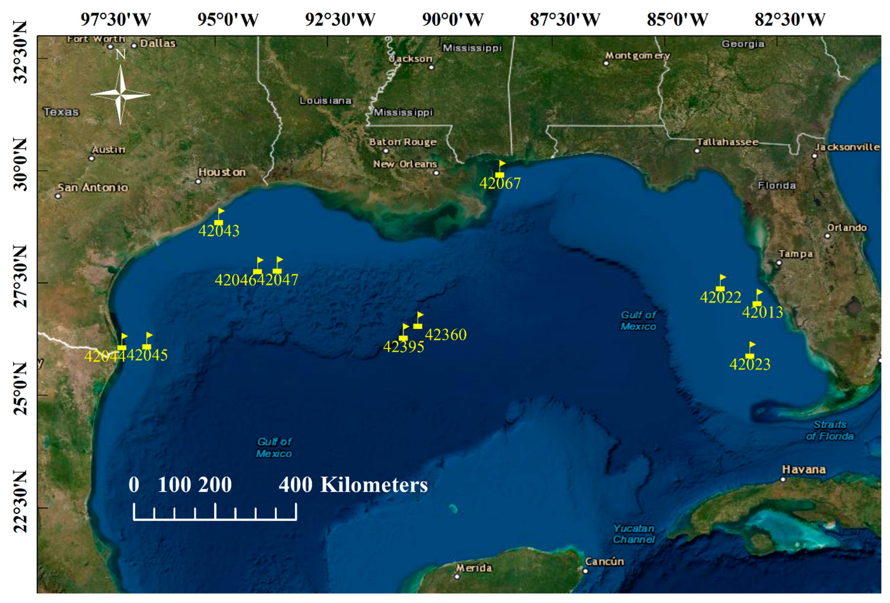
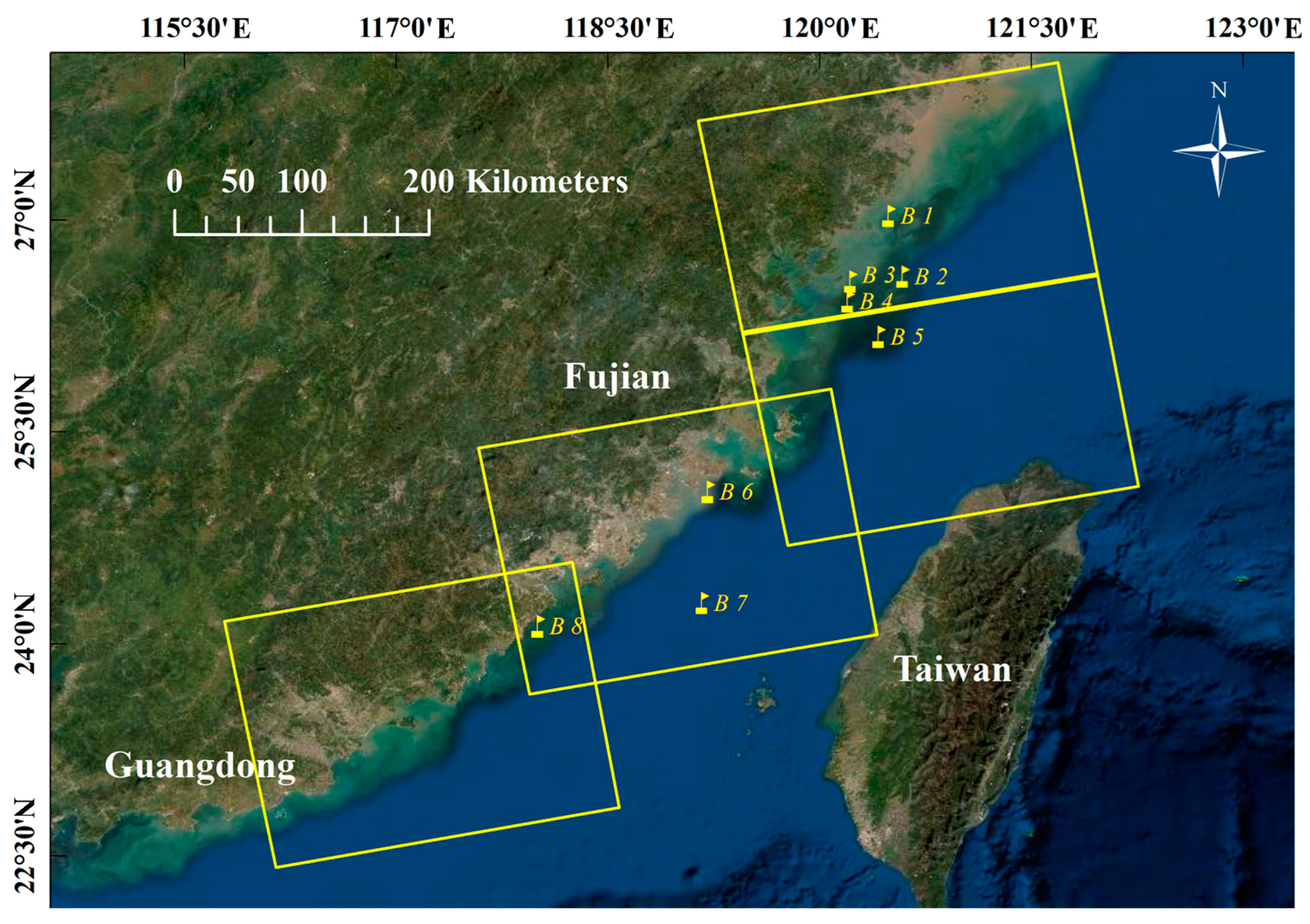
2.1.3. In Situ Buoy Data

Five-year ASCAT measurements and in situ wind data from the National Data Buoy Center (NDBC) buoys provided by National Oceanic and Atmospheric Administration (NOAA) are collocated and used to train the OPEN model. The 11 moored buoys are mainly near the coast and located around the Gulf of Mexico (as shown in Figure 1). The wind data are averaged over a period of 8.5 min [48].
To illustrate the capability of the OPEN method for wind retrieval for distinct sea states and topography, buoy data from October 2019 to April 2020 near the coasts of Fujian Province, in the East China Sea, is used as an independent data set to validate the proposed wind retrieval method. The adjacent sea has a mean water depth of ~60 m [49], an intensified wind jet in winter with wind speed >10 m/s [50], and resultant high sea states. Therefore, it is a question to be answered to what extent the method can be applied in wind retrieval for distinct environments. These data are provided by the Fujian provincial meteorological bureau. Figure 2 shows the location of these buoys and collocated SAR data. The distance from all buoys to the coastal lines is more than 5 km to reduce the influence of land. Table 1 lists the information of buoy data used in this research.
Because buoy anemometers are at different heights above the sea surface, wind speeds have been corrected to a reference level of 10 m for training and comparing with measured satellite data. It should be mentioned that by considering boundary-layer stratifications or not, radar sensors can provide neutral and nonneutral winds. By further accounting for the effects of air mass density, equivalent neutral winds can be corrected to stress-equivalent winds. Recent work has shown that the satellite-derived winds can be improved using stress-equivalent winds accounting for the effects of atmospheric stability [26]. However, calculations of stress-equivalent winds require the information of air mass density (related to the sea surface temperature, sea surface pressure, and humidity), which cannot be simultaneously provided by the buoys used in this study. Therefore, we follow Bidlot et al. [51] to use the steady-state neutral wind profile relation to solve the friction velocity (u*). The wind speed (U, m/s) at a height of z (m) can be given by
U(z) = u*ln(z/z0)/κ
z0 = αu*2/g,
where κ is the von Karman constant of 0.41, α is the constant Charnock parameter, and g is the acceleration of gravity.

2.2. Collocated Satellite Data and Buoy Observations

The ASCAT coastal wind products are spatially and temporally collocated with in situ NDBC buoy measurements within the distance of 12.5 km and the time window of 30 min. Considering that very low wind speeds from C-band radars may not be reliable due to the absence of Bragg waves [52], buoy measurements with wind speeds less than 1 m/s are abandoned in the collocated dataset. The middle-beam sea surface radar backscatter σ0, incidence angle, and radar look azimuth, which are extracted from ASCAT acquisitions, are subsequently collocated with wind vectors from buoys. The incidence angles of collocated ASCAT data range from 26.81° to 52.79°. The histogram using 53,406 collocated data from buoy observations is shown in Figure 3. The wind speeds range from about 1 m/s to 18 m/s. The collocated data sets from ASCAT and NDBC buoy observations are randomly separated into two sets. Among the collocated data, 98% of points are randomly selected as the training set, and the remaining 2% are taken as the test set for assessing the performance of the OPEN model.
To further validate the proposed method using NDBC data against an independent data set from Chinese buoys, a collocated data set is also generated by collocated Sentinel-1 SAR data and buoy observations in the East China Sea. Exclusively, 28 images collected from four repeated orbits are collocated with the buoys near Fujian (locations are shown in Figure 2). The collocated observations between the buoy and SAR occurred within 10 min and a 1 km radius. This process provides a total of 71 collocated points (including the wind speed, wind direction, C-band NRCS in VV polarization, incidence angle, and radar look angle).

2.3. The CMOD Functions

C-band GMFs have been widely used to obtain the sea surface wind field for C-band SAR. It can thus provide another good reference to evaluate the performance of the OPEN method. In this study, CMOD4, CMOD-IFR2, CMOD5.N, and CMOD7 are chosen for the cross-validation. The CMOD model is an empirical function, which can be described as:
σ0 = B0(1 + B1 cos ϕ + B2 cos 2ϕ)p,
where σ0 is the NRCS in VV polarization. B0, B1, and B2 are functions of incidence angle (θ) and U10. ϕ is the relative angle between wind direction (WD) and radar look azimuth (RLA). p is a parameter, which can be chosen as 1.6 to avoid higher order harmonic terms in CMOD4 and CMOD5.N. The formulation of CMOD7 is a look-up table, which can be obtained from the website of KNMI (https://scatterometer.knmi.nl/cmod7/ accessed on 1 February 2022).

2.4. Development of the OPEN Method

The NN-based OPEN method is detailed in [40,41], while here we only present some necessary information. We adopt a NN with 2 hidden layers, each with 30 neurons. The structure of the OPEN model is presented in Figure 4. One may argue that using a deep NN could better capture the nonlinear relationship between the input and output data. However, given the sample size of ~53,400, training a deep NN is an unrealistic practice. For simplifying the calculation, we tend to use a shallow and relatively wide NN for the retrieval. Theoretically, an NN with sufficient neurons can approximate any continuous function, which is known as the universal approximation theorem [53]. Our practice suggested that the Bayesian regularization algorithm can efficiently avoid overfitting by adding some degree of smoothness to the cost function [54]. The input features of the NN model include σ0 in VV polarization (dB), θ (in degree), wind direction (in degree from 0° to 360°), and radar azimuth angle (in degree from 0° to 360°). In practice, wind directions for SAR wind speed retrieval can be typically obtained from external wind inputs, such as atmospheric models [37] or wind-induced streaks [55]. Wind directions from the ECMWF model will be used in the OPEN model to present the distribution of SAR winds in the East China Sea in Section 3.
The root-mean-squared error (RMSE), correlation coefficient (R), mean absolute percentage error (MAPE), and bias are used to evaluate the wind results in this research. Because an explicit cross-validation subset is not required to ensure generalization based on the Bayesian Regularization algorithm, 98% of the collocated data (52,337 points) are randomly selected as the training set. The colormap represents the sample counts. The comparison between the OPEN results and labeled wind data from NDBC buoy measurements can be seen in Figure 5. The relatively small RMSE (less than 1.2 m/s) and bias (less than 0.01 m/s) indicate that the OPEN model fits the label wind data well.

3. Results

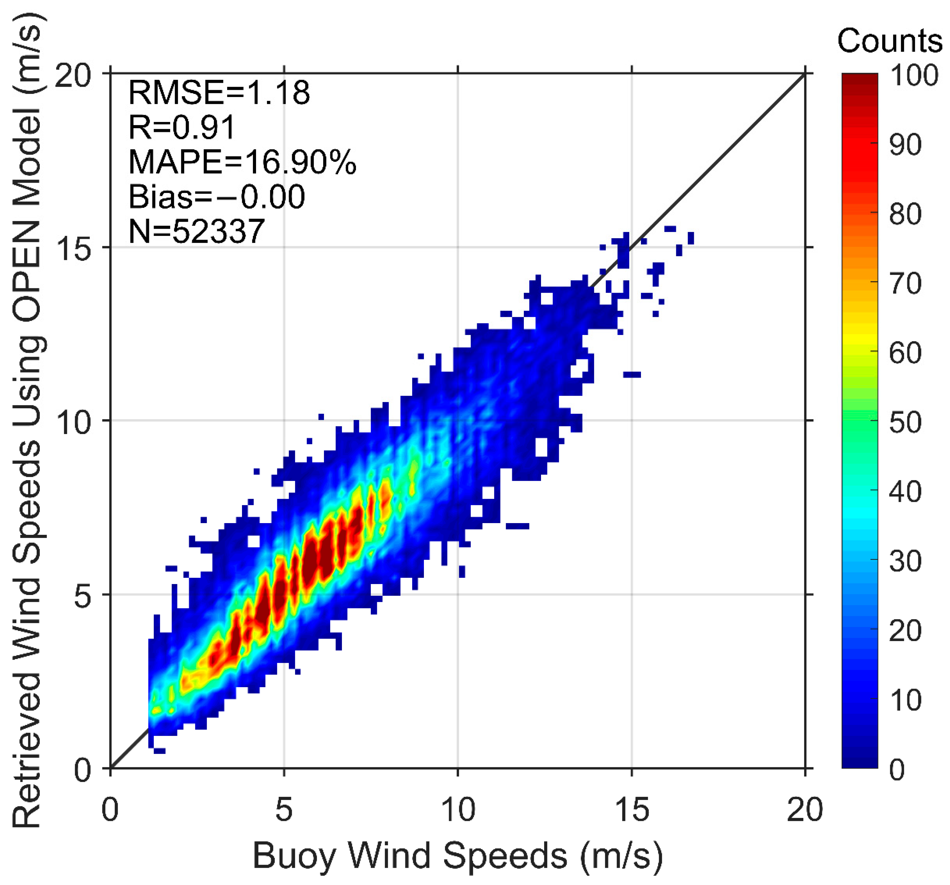
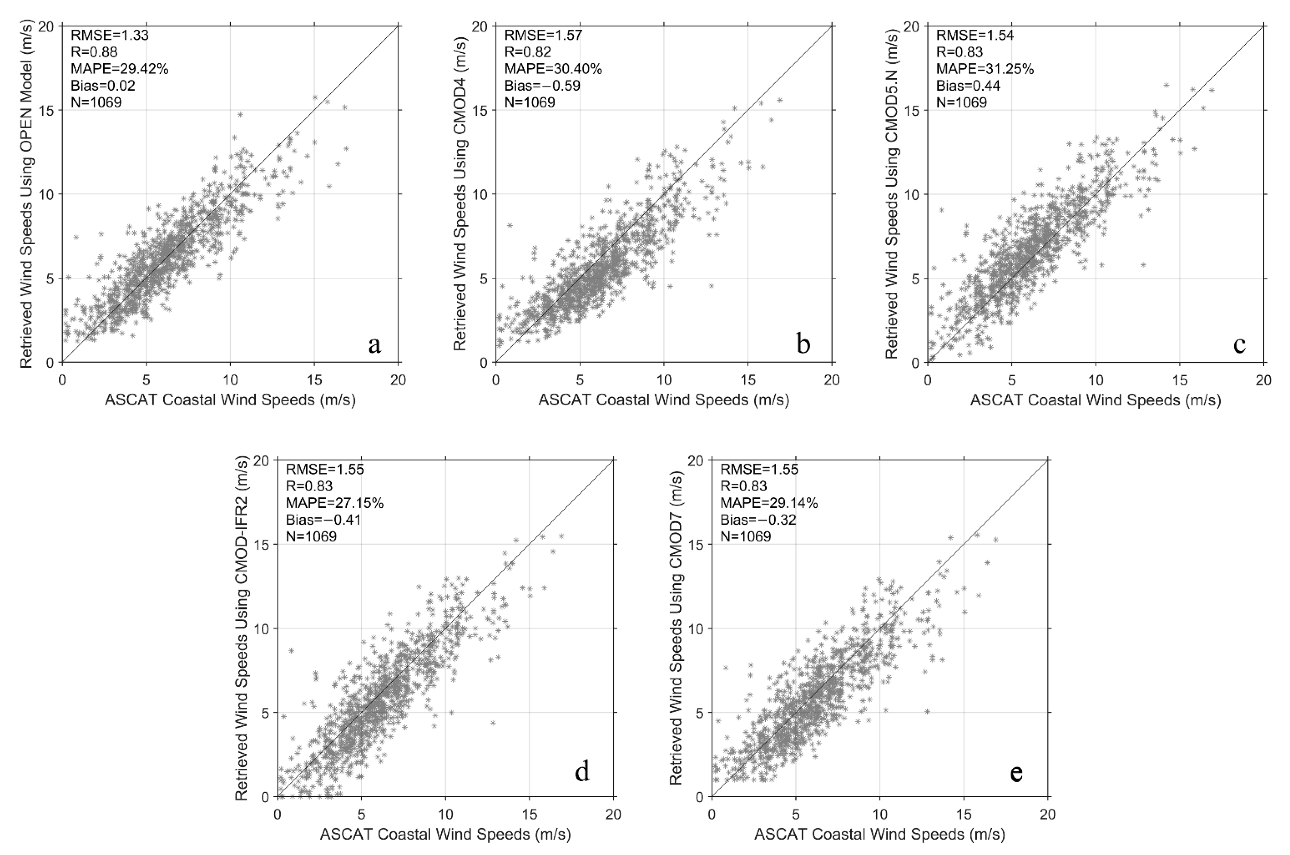
3.1. Evaluation of the Wind Speed Estimation from ASCAT Data

The accuracy of wind retrievals by the OPEN method is first validated by the test data set using the remaining 2% points. The incidence angle, NRCS in VV polarization, radar azimuth angle from ASCAT data, and the actual wind direction from the NDBC buoys are regarded as the input to the NN model to retrieve the sea surface wind speeds. CMOD4, CMOD5.N, CMOD-IFR2, and CMOD7 are used to compare the U10 obtained from the OPEN method. Note that the CMOD4 is tuned for nonneutral wind, while CMOD-IFR2, CMOD5.N, and the OPEN model can provide neutral winds. The latest CMOD7 can provide stress-equivalent winds after a correction of air mass density and stability [26]. The global average neutral wind is slightly larger (~0.2 m/s) than the nonneutral wind [20], which may also influence the model results. The comparison between these model results and collocated buoy measurements can be seen in Figure 6. It shows that the derived wind speed by our NN model is in good agreement with NDBC buoy measurements with an RMSE of 1.15 m/s, a correlation coefficient of 0.91, a MAPE of 17.2%, and a bias of 0.02 m/s in Figure 6a. The CMOD functions perform similarly but share a larger RMSE (approximately 1.5 m/s) and correlation coefficient (around 0.84) compared with NDBC buoys, which is outperformed by the OPEN model.
Since ASCAT wind retrievals are a high scientific level operational product with high quality, it is exploited to assess the accuracy of the proposed model. The statistical validations are also carried out using the test data, which are shown in Figure 7. Compared with ASCAT coastal wind products, the results show that the RMSE and bias of the OPEN model are both the smallest one, while the CMOD7 model can obtain a smaller MAPE and bias than other C-band GMFs as expected because CMOD4 and CMOD5.N are predecessors of CMOD7 for operational ASCAT winds.

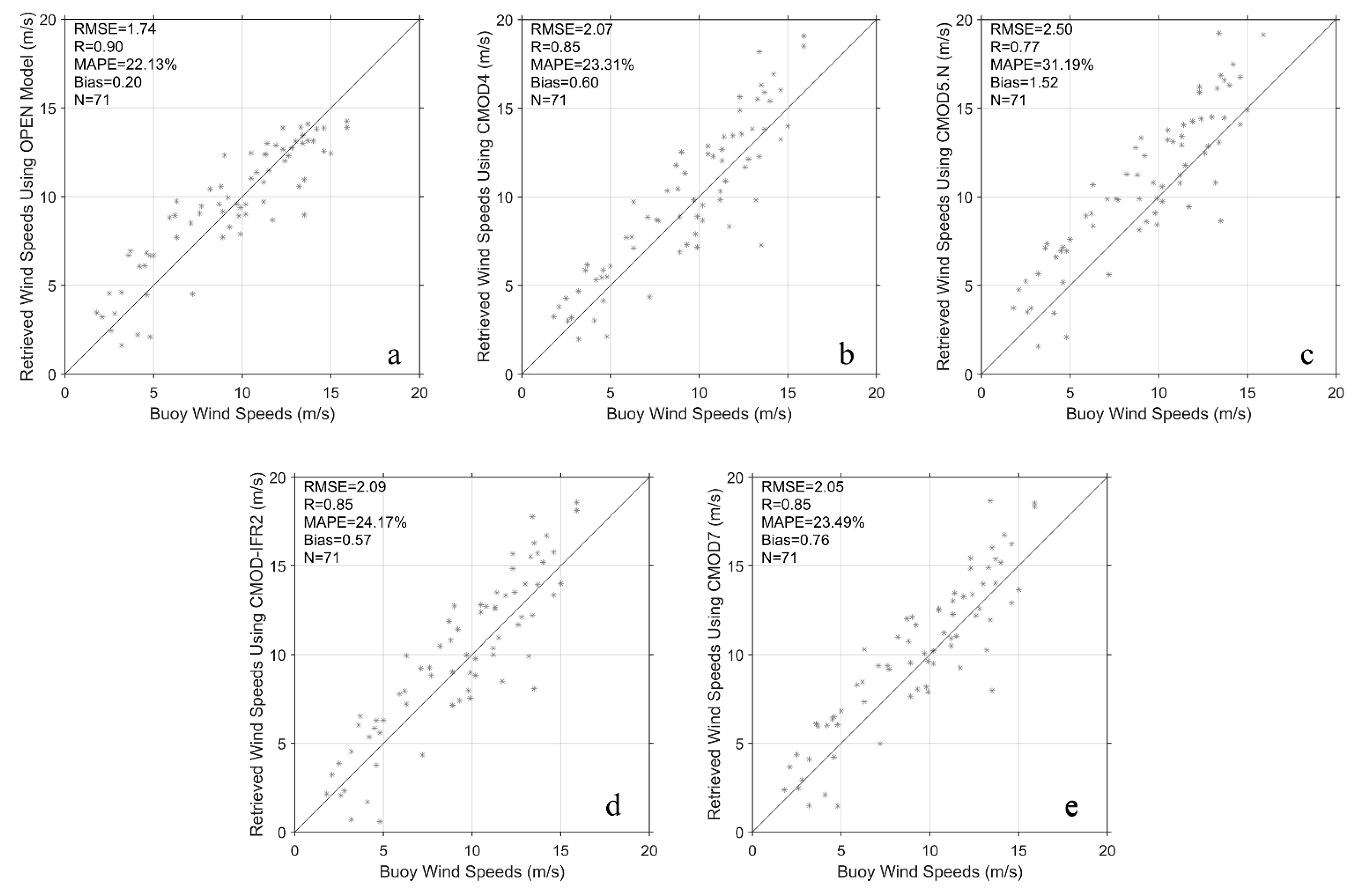
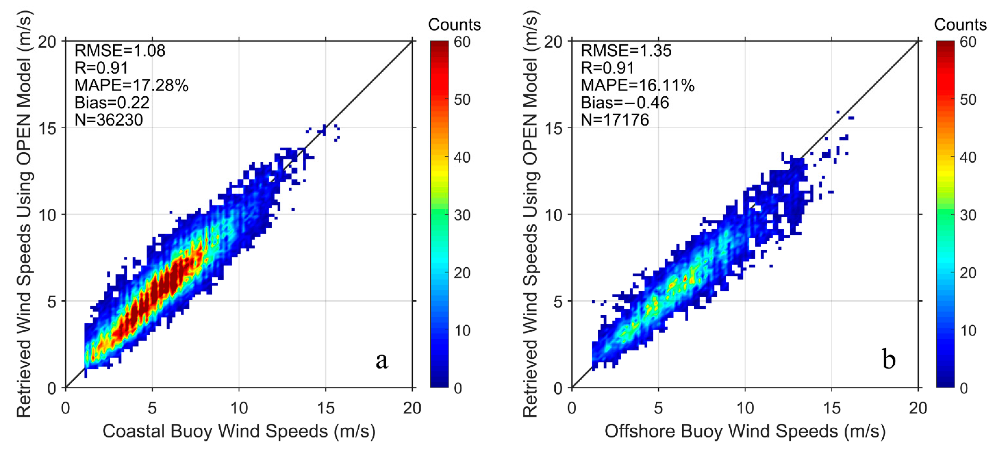
3.2. Evaluation of the Wind Speed Estimation from SAR Data

The performance of the OPEN model is further assessed using C-band Sentinel-1 SAR data and in situ wind measurements from buoys near the coast of Fujian, China (as shown in Figure 2). The σ0, incidence angle, azimuth angle from SAR data together with the wind direction from coastal buoys are used to obtain the sea surface wind speed using the OPEN model, CMOD4, CMOD5.N, CMOD-IFR2, and CMOD7. Figure 8 shows the comparisons of buoy and SAR wind speeds using these five models. Overall, the OPEN model can acquire better results (RMSE and correlation coefficient) compared with the CMOD functions. The accuracy of wind speeds (RMSE) by the NN model (1.74 m/s) is still better than the CMOD functions with 2.07 m/s (CMOD4), 2.5 m/s (CMOD5.N), 2.09 m/s (CMOD-IFR2), and 2.05 m/s (CMOD7). As for the bias, the OPEN model obtains a smaller bias compared with the other four CMOD functions, and the CMOD4, CMOD-IFR2, and CMOD7 functions perform similarly. The CMOD5.N model obviously overestimates the wind speed for ~1.5 m/s.

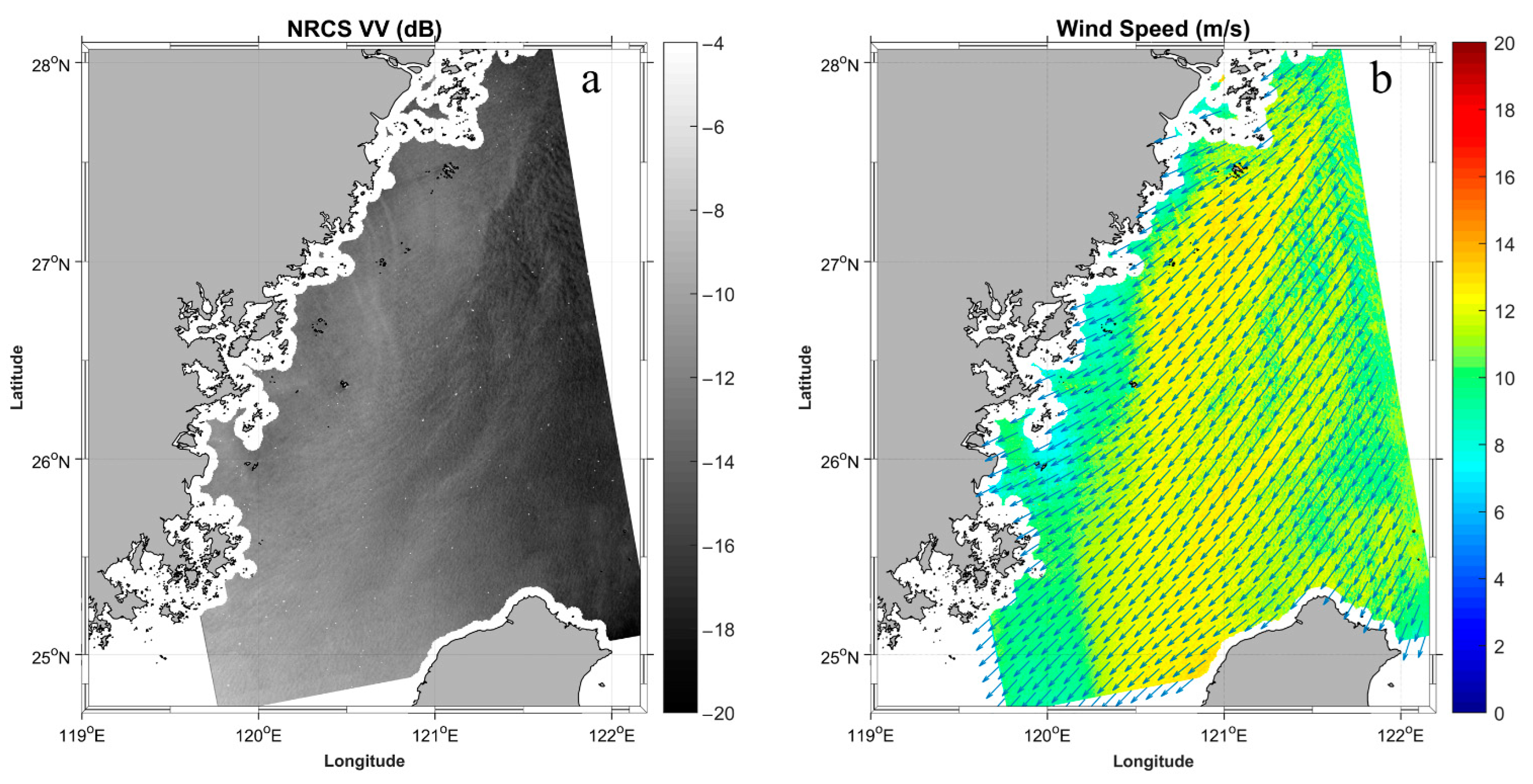
3.3. SAR-Derived Wind Map Using the OPEN Model

As an example, an image showing the near sea surface wind speeds estimated from the proposed model is further analyzed using the SAR image that was obtained from Sentinel-1 on 12 January 2020. Two SAR images (over the same region as shown in the northeast of Figure 2) with a time interval of around 25 s are merged to present a larger coverage area in Figure 9a. The collocated wind speeds retrieved from the OPEN model using SAR parameters and wind directions from the ECMWF forecast model can be seen in Figure 9b. The spatial resolution of the estimated wind speeds is the same as the processed SAR image, with 1 km, while the grid spacing is interpolated to be approximately 9 km for the ECMWF wind directions to provide a better view. The acquired time of the image is in a cold season during the winter monsoon with a mean wind speed of around 11.05 m/s and prevailing winds from the northeast. For this region of the East China Sea in winter, southward Chinese Coastal Currents are often observed, which bring cold water to this area [56]. In response to the cross-shore gradient of the sea surface temperature, several localized air–sea interaction mechanisms [57] have been involved to generate along-shore strips of high wind speeds. Overall, the obtained wind field in Figure 9b is quite smooth, and no outliers are found.

4. Discussion

The complicated nonlinear relationship between observed sea surface radar backscatter and wind vectors is solved using the OPEN method. Instead of using reanalysis wind data or model results, in situ wind observations exclusively from buoys near the coasts are used as the label data for training the NN model based on five-year C-band NRCS measurements. Compared with operational GMFs, the NN-based model does not rely on the empirical cosine-type equation as shown in Equation (3). For instance, ϕ (the relative angle between radar look azimuth and wind direction) does not need to be calculated in this study, and these two direction parameters can be separately input into the OPEN model to obtain wind speeds.
It can be found from Figure 8 that the four CMOD functions do not perform well for the estimates of coastal SAR winds with RMSEs of more than 2 m/s, especially for the CMOD5 model with the bias and RMSE of around 1.5 m/s and 2.5 m/s. Even an absolute NRCS calibration accuracy of about 0.5 dB cannot explain this bias (less than 0.5 m/s for moderate incidence angles and low to moderate wind speeds [52]). The OPEN model can obtain a smaller RMSE of about 1.74 m/s in Figure 8a, but it is worse than the result from the test ASCAT data (around 1.15 m/s in Figure 6a). What are the sources of errors? Apart from radar geometries and NRCS processing, it was reported that the wind direction [58], water depth [18], and other sea state factors [59,60] can influence sea surface wind measurements from SAR satellites, especially in coastal areas. The error from the direction should be small because the input direction in Figure 6 and Figure 8 are obtained from in situ buoy data. However, our analysis in Figure 9 uses external wind directions from the model winds for the SAR wind speed retrieval. Recent research has shown that the real spatial resolution of ECMWF winds is more than 100 km [27], which can bring in representativeness errors obtained from differences in spatial resolution when using model wind directions for SAR wind speed retrieval.
The collocated training and NDBC buoy data are divided into two parts according to water depth. Observations with water depth less than 100 m are regarded as coastal winds with 36,230 points, and the remaining data with 17,176 points are presented as offshore winds shown in Figure 10. The comparisons between the ASCAT 12.5 km coastal wind product and buoy data have indicated that the quality of the coastal winds can be as good as for the offshore winds [45]. Similar results can also be seen by using the OPEN model. Although the RMSE of offshore winds (1.35 m/s) is larger than coastal winds (1.08 m/s), similar MAPEs between OPEN model results and in situ measured data are found with values of 16.11% for offshore winds and 17.28% for coastal winds, which indicates that the proposed model performs similar for coastal and offshore winds in the Gulf of Mexico. However, for the coastal area near Fujian, the overall water depth is much shallower than those of the Gulf of Mexico. The difference in water depth and coastlines could lead to very different sea state factors. In terms of the waves, higher significant wave height can be found in the Taiwan Strait (~1.6–2.1 m) [61] than in the Gulf of Mexico (~1.2 m) [62]. Except for waves, many other factors can result in the deviation in derived winds, e.g., different climates, sea surface temperature, wind conditions, etc. For instance, the proposed model does not remove the effect of air mass density and air mass stability. A correction to the stress-equivalent reference winds has shown its benefit for ASCAT winds using information of the sea surface temperature, sea surface pressure and humidity [26]. After an ocean calibration, the retrieved winds by CMOD models can also be improved [63]. The OPEN model performs better than other models, although this calibration process has not been applied to the training NRCS data to keep consistent with not well-calibrated SAR data.
Yet, the comparisons of MAPE for two validation subsets (22.13% for Fujian coastal buoys vs. 17.19% for the cross-validation set) suggest that the OPEN method performs similarly well. Even with limited observations, OPEN can correctly extract sea surface winds under different sea state conditions without complex processing of the training data. This highlights the potential of such neural network methods in surface wind retrieval with considerable extrapolating capabilities. Surely, much more independent observation would be required. Additional inclusions of the air mass density correction, ocean calibration, and other sea state effects in the NN-based model may also be of high importance to provide accurate wind speed estimates for C-band SAR in future efforts. The input wind direction for the NN model from alternative sources with a spatial resolution comparable to SAR should also be considered to provide more reliable results at a fine scale of less than 1 km.

5. Conclusions

In this research, a novel method based on the NN technique and Bayesian regularization algorithm is proposed to retrieve sea surface wind speed for C-band SAR sensors. In situ wind observations exclusively from buoy data, instead of reanalysis wind data or model results, are used as the reference winds to train the neural network based on five-year collocated data. Through the evaluation of derived wind speeds using ASCAT coastal wind products and coastal buoy data from different sources, the results show that the proposed OPEN model can work well for wind speed estimates.
Overall, the proposed approach based on the OPEN model is promising for single-antenna C-band SAR sensors. The retrieved wind fields with a fine spatial resolution derived from SAR are highly important for scientific and applied purposes. As small satellites and constellations develop rapidly, it is also expected that CubeSat and small satellite SAR-based missions will strengthen the use of high-resolution radar data together with the NN model for providing continuous and accurate ocean wind information.

Author Contributions

Conceptualization, P.Y., J.A.J. and W.L.; methodology, W.X. and W.L.; validation, P.Y., W.X. and X.Z.; formal analysis, X.Z. and Y.H.; investigation, P.Y., X.G. and W.L.; data curation, P.Y.; writing—original draft preparation, P.Y.; writing—review and editing, P.Y., X.Z., J.A.J., X.G. and W.L.; visualization, X.G. and Y.H.; supervision, J.A.J., X.-H.Y. and W.L. All authors have read and agreed to the published version of the manuscript.

Funding

This research was funded by the National Natural Science Foundation of China (grant numbers 41906184 and 41906019); the Natural Science Foundation of Fujian Province (grant numbers 2020J05232 and 2020J01263); the Key Laboratory of Spatial Data Mining & Information Sharing of Ministry of Education, Fuzhou University (2022LSDMIS07); the Fujian Province Construction Technology Research and Development Project (2020-K-60). The study is also supported by the National Key R&D Program of China (2019YFA0606702), the National Natural Science Foundation of China (Grant Numbers‪: 91858202, 41630963, and 41776003‪). X.-H.Y. has been supported by NSF (IIS-2123264) and NASA (80NSSC20M0220). X.G. is supported by Industry-University Cooperation and Collaborative Education Project (202102245034).

Institutional Review Board Statement

Not applicable.

Informed Consent Statement

Not applicable.

Data Availability Statement

Sentinel-1 data are freely available on the Copernicus Open Access Hub at https://scihub.copernicus.eu/ (last access on 1 December 2021). The ASCAT data are available on the website of EUMETSAT at https://data.eumetsat.int/ (last access on 15 November 2021). The buoy data can be downloaded from the website of NDBC at https://www.ndbc.noaa.gov/ (last access on 1 December 2021). Other data presented in this study are available on request from the corresponding author.

Acknowledgments

The authors would like to thank the ESA, EUMETSAT, and NOAA for the provision of Sentinel-1 SAR, ASCAT, and NDBC buoy data. The first author thanks Anton Verhoef from KNMI for his support with ASCAT data processing. Support from the European Space Agency under the ESA-MOST Dragon program is also appreciated.

Conflicts of Interest

The authors declare no conflict of interest.

References

  1. Gerling, T.W. Structure of the surface wind field from the Seasat SAR. J. Geophys. Res. Earth Surf. 1986, 91, 2308–2320. [Google Scholar] [CrossRef]
  2. Allahdadi, M.N.; Gunawan, B.; Lai, J.; He, R.; Neary, V.S. Development and validation of a regional-scale high-resolution unstructured model for wave energy resource characterization along the US East Coast. Renew. Energy 2019, 136, 500–511. [Google Scholar] [CrossRef]
  3. Hegermiller, C.A.; Warner, J.C.; Olabarrieta, M.; Sherwood, C.R. Wave–Current Interaction between Hurricane Matthew Wave Fields and the Gulf Stream. J. Phys. Oceanogr. 2019, 49, 2883–2900. [Google Scholar] [CrossRef]
  4. Lu, W.; Yan, X.-H.; Jiang, Y. Winter bloom and associated upwelling northwest of the Luzon Island: A coupled physical-biological modeling approach. J. Geophys. Res. Oceans 2014, 120, 533–546. [Google Scholar] [CrossRef]
  5. Wang, T.; Yu, P.; Wu, Z.; Lu, W.; Liu, X.; Li, Q.P.; Huang, B. Revisiting the Intraseasonal Variability of Chlorophyll-a in the Adjacent Luzon Strait with a New Gap-Filled Remote Sensing Data Set. IEEE Trans. Geosci. Remote Sens. 2022, 60, 1–11. [Google Scholar] [CrossRef]
  6. Sempreviva, A.M.; Barthelmie, R.J.; Pryor, S.C. Review of Methodologies for Offshore Wind Resource Assessment in European Seas. Surv. Geophys. 2008, 29, 471–497. [Google Scholar] [CrossRef]
  7. Doubrawa, P.; Barthelmie, R.J.; Pryor, S.C.; Hasager, C.B.; Badger, M.; Karagali, I. Satellite winds as a tool for offshore wind resource assessment: The Great Lakes Wind Atlas. Remote Sens. Environ. 2015, 168, 349–359. [Google Scholar] [CrossRef] [Green Version]
  8. Wan, Y.; Guo, S.; Li, L.; Qu, X.; Dai, Y. Data Quality Evaluation of Sentinel-1 and GF-3 SAR for Wind Field Inversion. Remote Sens. 2021, 13, 3723. [Google Scholar] [CrossRef]
  9. Moon, W.M.; Staples, G.; Kim, D.-J.; Park, S.-E.; Park, K.-A. RADARSAT-2 and Coastal Applications: Surface Wind, Waterline, and Intertidal Flat Roughness. Proc. IEEE 2010, 98, 800–815. [Google Scholar] [CrossRef]
  10. Xu, Q.; Li, Y.; Li, X.; Zhang, Z.; Cao, Y.; Cheng, Y. Impact of Ships and Ocean Fronts on Coastal Sea Surface Wind Measure-ments from the Advanced Scatterometer. IEEE J. Sel. Top. Appl. Earth Obs. Remote Sens. 2018, 11, 2162–2169. [Google Scholar] [CrossRef]
  11. Zhang, B.; Perrie, W.; Zhang, J.A.; Uhlhorn, E.W.; He, Y. High-Resolution Hurricane Vector Winds from C-Band Du-al-Polarization SAR Observations. J. Atmos. Ocean. Technol. 2014, 31, 272–286. [Google Scholar] [CrossRef]
  12. Monaldo, F.; Jackson, C.; Li, X.; Pichel, W.G. Preliminary Evaluation of Sentinel-1A Wind Speed Retrievals. IEEE J. Sel. Top. Appl. Earth Obs. Remote Sens. 2016, 9, 2638–2642. [Google Scholar] [CrossRef]
  13. Wang, H.; Yang, J.; Mouche, A.; Shao, W.; Zhu, J.; Ren, L.; Xie, C. GF-3 SAR Ocean Wind Retrieval: The First View and Pre-liminary Assessment. Remote Sens. 2017, 9, 694. [Google Scholar] [CrossRef] [Green Version]
  14. Xue, S.; Geng, X.; Meng, L.; Xie, T.; Huang, L.; Yan, X.-H. HISEA-1: The First C-Band SAR Miniaturized Satellite for Ocean and Coastal Observation. Remote Sens. 2021, 13, 2076. [Google Scholar] [CrossRef]
  15. Stopa, J.E.; Mouche, A.A.; Collard, F.; Chapron, B. Sea State Impacts on Wind Speed Retrievals From C-Band Radars. IEEE J. Sel. Top. Appl. Earth Obs. Remote Sens. 2017, 10, 2147–2155. [Google Scholar] [CrossRef]
  16. Dagestad, K.F.; Horstmann, J.; Mouche, A.; Perrie, W.; Shen, H.; Zhang, B.; Li, X.; Monaldo, F.; Pichel, W.; Lehner, S.; et al. Wind retrieval from synthetic aperture radar—An overview. In Proceedings of the SEASAR 2012, Tromsø, Norway, 18–22 June 2012. [Google Scholar]
  17. Stoffelen, A.; Anderson, D. Scatterometer data interpretation: Estimation and validation of the transfer function CMOD4. J. Geophys. Res. Earth Surf. 1997, 102, 5767–5780. [Google Scholar] [CrossRef]
  18. Quilfen, Y.; Chapron, B.; Elfouhaily, T.; Katsaros, K.; Tournadre, J. Observation of tropical cyclones by high-resolution scat-terometry. J. Geophys. Res. Ocean. 1998, 103, 7767–7786. [Google Scholar] [CrossRef]
  19. Hersbach, H.; Stoffelen, A.; De Haan, S. An improved C-band scatterometer ocean geophysical model function: CMOD5. J. Geophys. Res. Earth Surf. 2007, 112, C03006. [Google Scholar] [CrossRef]
  20. Hersbach, H. Comparison of C-Band Scatterometer CMOD5.N Equivalent Neutral Winds with ECMWF. J. Atmos. Ocean. Technol. 2010, 27, 721–736. [Google Scholar] [CrossRef]
  21. Lu, Y.; Zhang, B.; Perrie, W.; Mouche, A.A.; Li, X.; Wang, H. A C-Band Geophysical Model Function for Determining Coastal Wind Speed Using Synthetic Aperture Radar. IEEE J. Sel. Top. Appl. Earth Obs. Remote Sens. 2018, 11, 2417–2428. [Google Scholar] [CrossRef] [Green Version]
  22. Mouche, A.; Chapron, B. Global C-Band Envisat, RADARSAT-2 and Sentinel-1 SAR measurements in copolarization and cross-polarization. J. Geophys. Res. Ocean. 2015, 120, 7195–7207. [Google Scholar] [CrossRef] [Green Version]
  23. Stiles, B.W.; Dunbar, R.S. A Neural Network Technique for Improving the Accuracy of Scatterometer Winds in Rainy Condi-tions. IEEE Trans. Geosci. Remote Sens. 2010, 48, 3114–3122. [Google Scholar] [CrossRef]
  24. Zhang, B.; Lu, Y.; Perrie, W.; Zhang, G.; Mouche, A. Compact Polarimetry Synthetic Aperture Radar Ocean Wind Retrieval: Model Development and Validation. J. Atmos. Ocean. Technol. 2021, 38, 747–757. [Google Scholar] [CrossRef]
  25. Stoffelen, A.; Verspeek, J.A.; Vogelzang, J.; Verhoef, A. The CMOD7 Geophysical Model Function for ASCAT and ERS Wind Retrievals. IEEE J. Sel. Top. Appl. Earth Obs. Remote Sens. 2017, 10, 2123–2134. [Google Scholar] [CrossRef]
  26. De Kloe, J.; Stoffelen, A.; Verhoef, A. Improved Use of Scatterometer Measurements by Using Stress-Equivalent Reference Winds. IEEE J. Sel. Top. Appl. Earth Obs. Remote Sens. 2017, 10, 2340–2347. [Google Scholar] [CrossRef]
  27. Vogelzang, J.; Stoffelen, A. Quadruple Collocation Analysis of In-Situ, Scatterometer, and NWP Winds. J. Geophys. Res. Ocean. 2021, 126, e2021JC017189. [Google Scholar] [CrossRef]
  28. Polverari, F.; Portabella, M.; Lin, W.; Sapp, J.W.; Stoffelen, A.; Jelenak, Z.; Chang, P.S. On High and Extreme Wind Calibration Using ASCAT. IEEE Trans. Geosci. Remote Sens. 2021, 60, 1–10. [Google Scholar] [CrossRef]
  29. Funahashi, K.-I. On the approximate realization of continuous mappings by neural networks. Neural Netw. 1989, 2, 183–192. [Google Scholar] [CrossRef]
  30. Chen, K.; Tzeng, Y.; Chen, P. Retrieval of ocean winds from satellite scatterometer by a neural network. IEEE Trans. Geosci. Remote Sens. 1999, 37, 247–256. [Google Scholar] [CrossRef]
  31. Li, X.; Liu, B.; Zheng, G.; Ren, Y.; Zhang, S.; Liu, Y.; Gao, L.; Liu, Y.; Zhang, B.; Wang, F. Deep-learning-based information mining from ocean remote-sensing imagery. Natl. Sci. Rev. 2020, 7, 1584–1605. [Google Scholar] [CrossRef]
  32. Thiria, S.; Mejia, C.; Badran, F.; Crépon, M. A neural network approach for modeling nonlinear transfer functions: Application for wind retrieval from spaceborne scatterometer data. J. Geophys. Res. Earth Surf. 1993, 98, 22827–22841. [Google Scholar] [CrossRef]
  33. Cornford, D.; Nabney, I.; Bishop, C.M. Neural Network-Based Wind Vector Retrieval from Satellite Scatterometer Data. Neural Comput. Appl. 1999, 8, 206–217. [Google Scholar] [CrossRef]
  34. Evans, D.J.; Cornford, D.; Nabney, I. Structured neural network modelling of multi-valued functions for wind vector retrieval from satellite scatterometer measurements. Neurocomputing 2000, 30, 23–30. [Google Scholar] [CrossRef] [Green Version]
  35. Lin, M.; Song, X.; Jiang, X. Neural network wind retrieval from ERS-1/2 scatterometer data. Acta Oceanol. Sin. 2006, 25, 35–39. [Google Scholar]
  36. Horstmann, J.; Schiller, H.; Schulz-Stellenfleth, J.; Lehner, S. Global wind speed retrieval from sar. IEEE Trans. Geosci. Remote Sens. 2003, 41, 2277–2286. [Google Scholar] [CrossRef] [Green Version]
  37. Shao, W.; Zhu, S.; Zhang, X.; Gou, S.; Jiao, C.; Yuan, X.; Zhao, L. Intelligent Wind Retrieval from Chinese Gaofen-3 SAR Im-agery in Quad Polarization. J. Atmos. Ocean. Technol. 2019, 36, 2121–2138. [Google Scholar] [CrossRef]
  38. Qin, T.; Jia, T.; Feng, Q.; Li, X. Sea surface wind speed retrieval from Sentinel-1 HH polarization data using conventional and neural network methods. Acta Oceanol. Sin. 2021, 40, 13–21. [Google Scholar] [CrossRef]
  39. Li, X.-M.; Qin, T.; Wu, K. Retrieval of Sea Surface Wind Speed from Spaceborne SAR over the Arctic Marginal Ice Zone with a Neural Network. Remote Sens. 2020, 12, 3291. [Google Scholar] [CrossRef]
  40. Lu, W.; Su, H.; Yang, X.; Yan, X.-H. Subsurface temperature estimation from remote sensing data using a clustering-neural network method. Remote Sens. Environ. 2019, 229, 213–222. [Google Scholar] [CrossRef]
  41. Su, H.; Zhang, H.; Geng, X.; Qin, T.; Lu, W.; Yan, X.-H. OPEN: A New Estimation of Global Ocean Heat Content for Upper 2000 Meters from Remote Sensing Data. Remote Sens. 2020, 12, 2294. [Google Scholar] [CrossRef]
  42. Masson-Delmotte, V.; Zhai, P.; Pirani, A.; Connors, S.L.; Péan, C.; Berger, S.; Caud, N.; Chen, Y.; Goldfarb, L.; Gomis, M.I.; et al. IPCC, Climate Change 2021: The Physical Science Basis; Contribution of Working Group I to the Sixth Assessment Report of the Intergovernmental Panel on Climate Change; Cambridge University Press: Cambridge, UK, 2021. [Google Scholar]
  43. Sun, Y.; Li, X.-M. Denoising Sentinel-1 Extra-Wide Mode Cross-Polarization Images Over Sea Ice. IEEE Trans. Geosci. Remote Sens. 2020, 59, 2116–2131. [Google Scholar] [CrossRef]
  44. Park, J.-W.; Won, J.-S.; Korosov, A.; Babiker, M.; Miranda, N. Textural Noise Correction for Sentinel-1 TOPSAR Cross-Polarization Channel Images. IEEE Trans. Geosci. Remote Sens. 2019, 57, 4040–4049. [Google Scholar] [CrossRef]
  45. Verhoef, A.; Portabella, M.; Stoffelen, A. High-Resolution ASCAT Scatterometer Winds Near the Coast. IEEE Trans. Geosci. Remote Sens. 2012, 50, 2481–2487. [Google Scholar] [CrossRef] [Green Version]
  46. Yu, P.; Johannessen, J.A.; Yan, X.; Geng, X.; Zhong, X.; Zhu, L. A Study of the Intensity of Tropical Cyclone Idai Using Dual-Polarization Sentinel-1 Data. Remote Sens. 2019, 11, 2837. [Google Scholar] [CrossRef] [Green Version]
  47. Schwerdt, M.; Schmidt, K.; Ramon, N.T.; Alfonzo, G.C.; Döring, B.; Zink, M.; Prats-Iraola, P. Independent Verification of the Sentinel-1A System Calibration. IEEE J. Sel. Top. Appl. Earth Obs. Remote Sens. 2015, 9, 994–1007. [Google Scholar] [CrossRef] [Green Version]
  48. Gilhousen, D.B. A Field Evaluation of NDBC Moored Buoy Winds. J. Atmos. Ocean. Technol. 1987, 4, 94–104. [Google Scholar] [CrossRef] [Green Version]
  49. Hong, H.; Chai, F.; Zhang, C.; Huang, B.; Jiang, Y.; Hu, J. An overview of physical and biogeochemical processes and ecosystem dynamics in the Taiwan Strait. Cont. Shelf Res. 2011, 31, S3–S12. [Google Scholar] [CrossRef]
  50. Lu, W.; Wang, J.; Jiang, Y.; Chen, Z.; Wu, W.; Yang, L.; Liu, Y. Data-Driven Method with Numerical Model: A Combining Framework for Predicting Subtropical River Plumes. J. Geophys. Res. Oceans 2022, 127, e2021JC017925. [Google Scholar] [CrossRef]
  51. Bidlot, J.-R.; Holmes, D.J.; Wittmann, P.A.; Lalbeharry, R.; Chen, H.S. Intercomparison of the Performance of Operational Ocean Wave Forecasting Systems with Buoy Data. Weather Forecast. 2002, 17, 287–310. [Google Scholar] [CrossRef]
  52. Yang, X.; Li, X.; Pichel, W.G.; Li, Z. Comparison of Ocean Surface Winds from ENVISAT ASAR, MetOp ASCAT Scatterometer, Buoy Measurements, and NOGAPS Model. IEEE Trans. Geosci. Remote Sens. 2011, 49, 4743–4750. [Google Scholar] [CrossRef]
  53. Hornik, K.; Stinchcombe, M.; White, H. Multilayer feedforward networks are universal approximators. Neural Netw. 1989, 2, 359–366. [Google Scholar] [CrossRef]
  54. Foresee, F.D.; Hagan, M.T. Gauss-Newton approximation to Bayesian learning. In Proceedings of the International Conference on Neural Networks (ICNN’97), Houston, TX, USA, 12 June 1997. [Google Scholar]
  55. Koch, W. Directional analysis of SAR images aiming at wind direction. IEEE Trans. Geosci. Remote Sens. 2004, 42, 702–710. [Google Scholar] [CrossRef]
  56. Liao, E.; Jiang, Y.; Li, L.; Hong, H.; Yan, X. The cause of the 2008 cold disaster in the Taiwan Strait. Ocean Model. 2012, 62, 1–10. [Google Scholar] [CrossRef]
  57. Oey, L.-Y.; Chang, M.-C.; Huang, S.-M.; Lin, Y.-C.; Lee, M.-A. The influence of shelf-sea fronts on winter monsoon over East China Sea. Clim. Dyn. 2015, 45, 2047–2068. [Google Scholar] [CrossRef]
  58. Portabella, M.; Stoffelen, A.; Johannessen, J.A. Toward an optimal inversion method for synthetic aperture radar wind retrieval. J. Geophys. Res. Earth Surf. 2002, 107, 1–13. [Google Scholar] [CrossRef]
  59. Plagge, A.M.; Vandemark, D.; Chapron, B. Examining the Impact of Surface Currents on Satellite Scatterometer and Altimeter Ocean Winds. J. Atmos. Ocean. Technol. 2012, 29, 1776–1793. [Google Scholar] [CrossRef]
  60. Krug, M.; Schilperoort, D.; Collard, F.; Hansen, M.; Rouault, M. Signature of the Agulhas Current in high resolution satellite derived wind fields. Remote Sens. Environ. 2018, 217, 340–351. [Google Scholar] [CrossRef]
  61. Cai, L.; Shang, S.; Wei, G.; He, Z.; Xie, Y.; Liu, K.; Zhou, T.; Chen, J.; Zhang, F.; Li, Y. Assessment of Significant Wave Height in the Taiwan Strait Measured by a Single HF Radar System. J. Atmos. Ocean. Technol. 2019, 36, 1419–1432. [Google Scholar] [CrossRef]
  62. Hwang, P.A.; Teague, W.J.; Jacobs, G.A.; Wang, D.W. A statistical comparison of wind speed, wave height, and wave period derived from satellite altimeters and ocean buoys in the Gulf of Mexico region. J. Geophys. Res. Earth Surf. 1998, 103, 10451–10468. [Google Scholar] [CrossRef] [Green Version]
  63. Rivas, M.B.; Stoffelen, A.; Verspeek, J.; Verhoef, A.; Neyt, X.; Anderson, C. Cone Metrics: A New Tool for the Intercomparison of Scatterometer Records. IEEE J. Sel. Top. Appl. Earth Obs. Remote Sens. 2017, 10, 2195–2204. [Google Scholar] [CrossRef] [Green Version]
Figure 1. Locations of the NDBC buoys for training the OPEN model in this study. The yellow marks indicate the locations of NDBC buoy data.
Remotesensing 14 02269 g001
Figure 2. Locations of the coastal buoys for the validation of SAR winds using the proposed model. The yellow rectangular box shows the locations of collocated SAR scenes, and the yellow marks indicate the locations of buoy data.
Remotesensing 14 02269 g002
Figure 3. Histogram of collocated in situ (a) wind speeds and (b) wind directions from NDBC buoys.
Remotesensing 14 02269 g003
Figure 4. Flowchart of the structure of the OPEN model.
Remotesensing 14 02269 g004
Figure 5. Comparison of OPEN model results and label wind data from buoy measurements.
Remotesensing 14 02269 g005
Figure 6. Comparisons of collocated NDBC buoy winds with retrieved wind speeds from the test data using (a) OPEN model, (b) CMOD4, (c) CMOD5.N, (d) CMOD-IFR2, and (e) CMOD7.
Remotesensing 14 02269 g006
Figure 7. Comparisons of collocated ASCAT coastal wind products with retrieved wind speeds from the test data using (a) OPEN model, (b) CMOD4, (c) CMOD5.N, (d) CMOD-IFR2, and (e) CMOD7.
Remotesensing 14 02269 g007
Figure 8. Comparisons of collocated coastal buoy winds with Sentinel-1 SAR winds using (a) OPEN, (b) CMOD4, (c) CMOD5.N, (d) CMOD-IFR2, and (e) CMOD7.
Remotesensing 14 02269 g008
Figure 9. (a) Sentinel-1 C-band SAR image in VV polarization that was acquired from the ascending pass at 10:02 UTC on 12 January 2020, given by the greyscale values (in dB); (b) wind speeds retrieved by the OPEN model, with the color bar denoting the wind speeds (m/s).
Remotesensing 14 02269 g009
Figure 10. Comparisons of retrieved winds using the OPEN model divided into (a) Coastal and (b) Offshore buoy wind speeds.
Remotesensing 14 02269 g010
Table 1. The information of buoy data used in this research.
Buoys in the Gulf of MexicoBuoys in the East China Sea
Station IDLatitudeLongitudeStation IDLatitudeLongitude
4201327.17°N82.92°WB1 (F3570)27.02°N120.50°E
4202227.50°N83.74°WB2 (58767)26.60°N120.59°E
4202326.01°N83.09°WB3 (F3520)26.56°N120.22°E
4204328.98°N94.90°WB4 (F3914)26.42°N120.21°E
4204426.19°N97.05°WB5 (58951)26.17°N120.42°E
4204526.22°N96.50°WB6 (F4325)25.07°N119.22°E
4204627.89°N94.04°WB7 (F0002)24.29°N119.17°E
4204727.90°N93.60°WB8 (59330)24.12°N118.01°E
4206730.04°N88.65°W
4236026.67°N90.47°W
4239526.40°N90.79°W
Publisher’s Note: MDPI stays neutral with regard to jurisdictional claims in published maps and institutional affiliations.

