
Combining Different Transformations of Ground Hyperspectral Data with Unmanned Aerial Vehicle (UAV) Images for Anthocyanin Estimation in Tree Peony Leaves


Abstract
:
1. Introduction
2. Materials and Methods
2.1. Study Area
2.2. Data Acquisition
2.2.1. Anth Quantification
2.2.2. Hyperspectral Data Acquisition
2.3. Airborne Campaigns
2.4. Pretreatment and Spectral Transformation of Ground-Based Spectrum
2.4.1. Principal Component Analysis (PCA) of Spectra
2.4.2. First-Order Differential (FD) Processing of Spectra
2.4.3. Continuum Removal Processing of Spectra
2.5. Unmanned Aerial Vehicles (UAV) Image Mosaic
2.5.1. RGB (Red-Green-Blue) Gray Vegetation Index Extraction
2.5.2. Texture Parameter Extraction of Unmanned Aerial Vehicle (UAV) Images
2.6. Regression Model Construction
2.7. Evaluation Index
3. Results
3.1. Characteristics of Spectrum
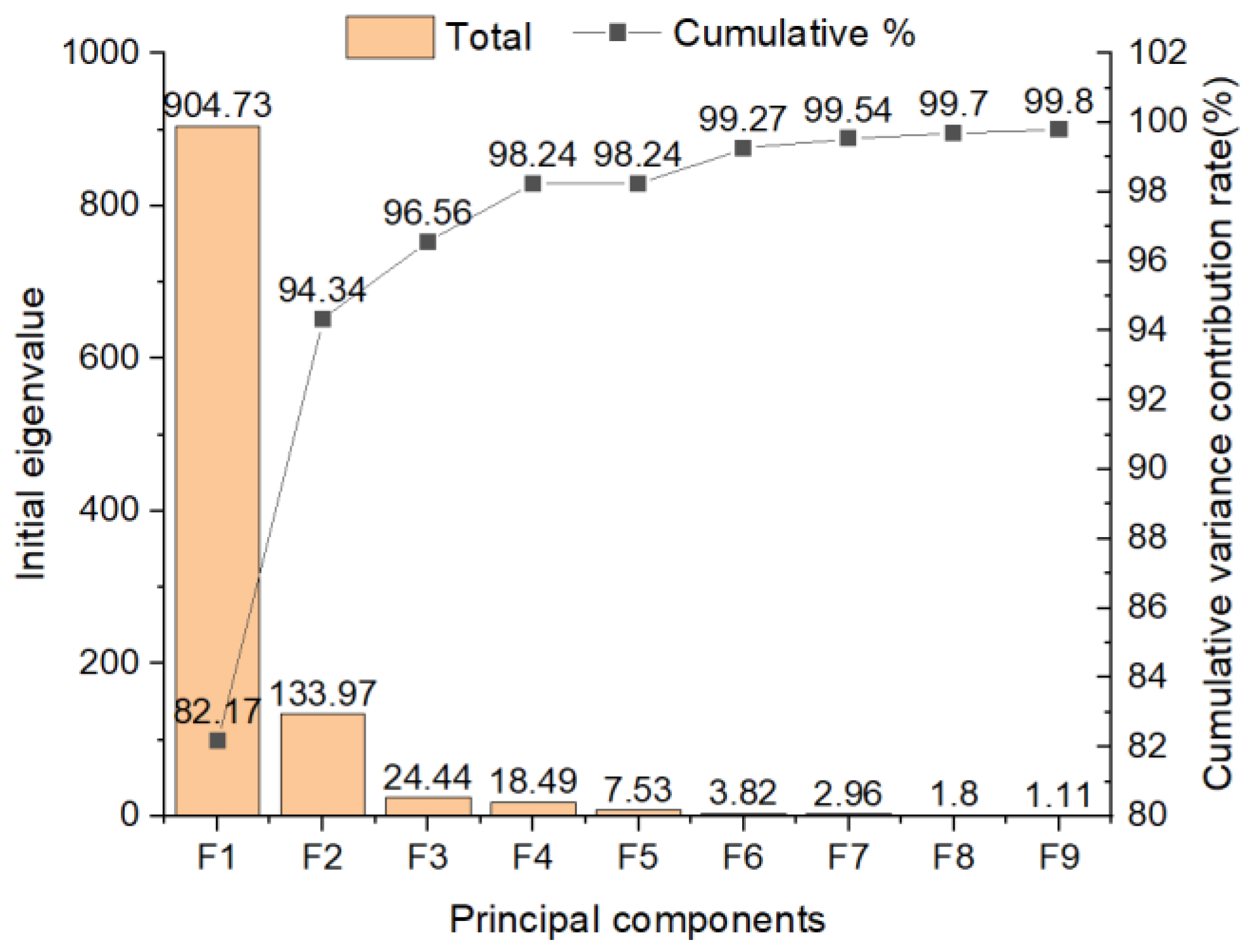
3.2. Principal Components of PCA Spectrum
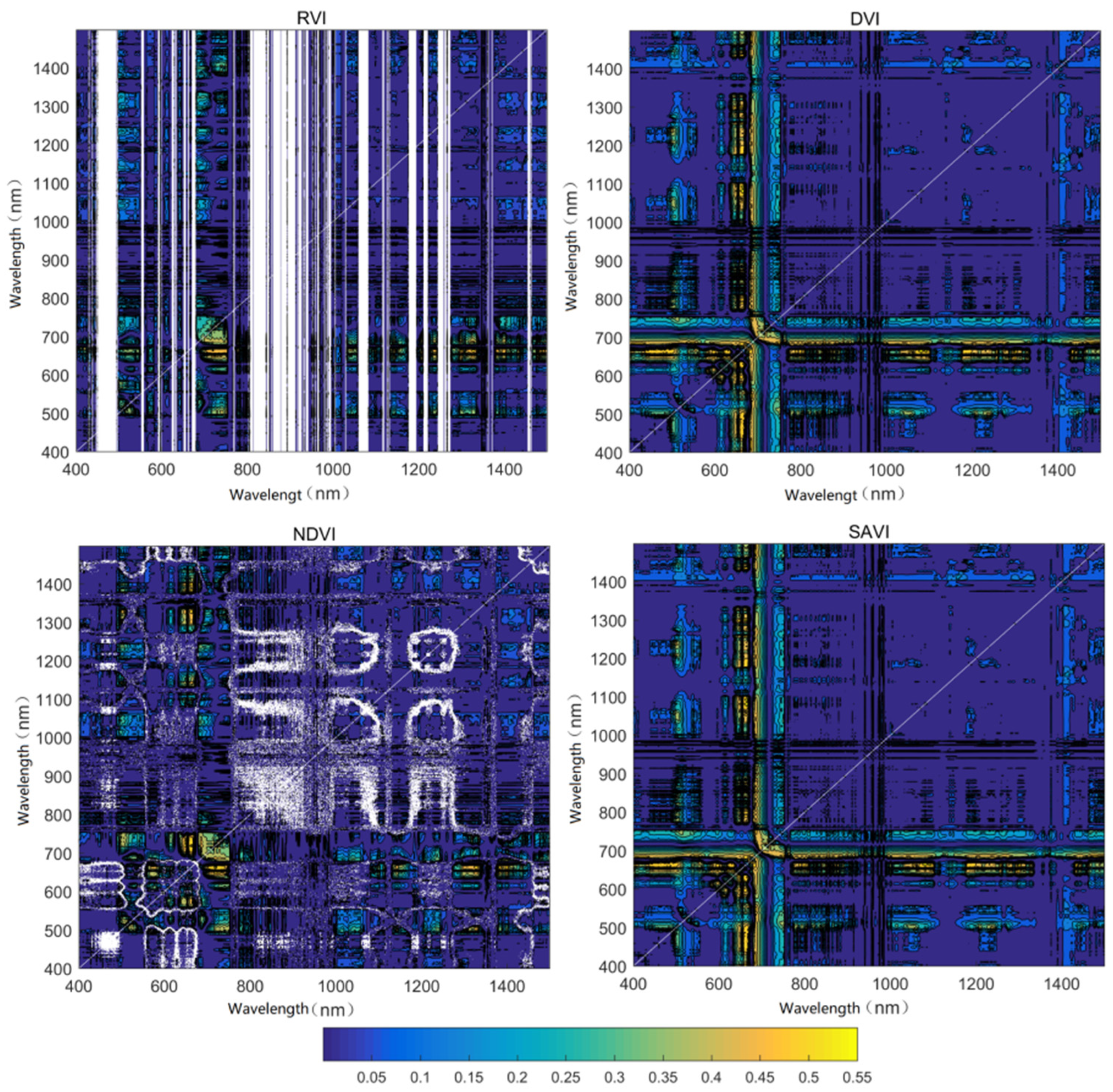
3.3. Vegetation Index of Any Two Bands of FD Spectrum
3.4. Correlation Analysis between Spectral Parameters and Anth
3.5. Correlation Analysis between Unmanned Aerial Vehicle (UAV) Parameters and Anth
3.6. Anth Estimation Based on Hyperspectral (HS) of Different Spectral Transformations
3.7. Anth Estimation Based on Unmanned Aerial Vehicle (UAV) Images
3.8. Anth Estimation Based on Multi-Source Remote Sensing (RS) Data
4. Discussion
4.1. Application of Spectral Information Extraction from Hyperspectral (HS) Data
4.2. Advantages of Ground-Based Spectrum and Unmanned Aerial Vehicle (UAV) Data
4.3. Machine Learning and Plant Growth Monitoring
5. Conclusions
- In the HS Anth estimation models constructed based on the three transformed spectra, the RF model based on “three-edge” parameters and VI of any two bands had the highest fitting accuracy, which can provide a reference for the selection of the spectral transformation method and regression model in crop growth monitoring in the future.
- Compared with the ground hyperspectral model and the visible UAV model, the accuracy of the multi-source RS models greatly improved. The addition of UAV data enriched the RS information used for near-surface estimation, which improved the accuracy of the model.
- Among the multi-source RS models, the RF model based on FD + UAV had the highest modeling and testing accuracy. It can thus be used for high-precision estimation of Anth in tree peony leaves.
Author Contributions
Funding
Data Availability Statement
Acknowledgments
Conflicts of Interest
References
- Landi, M.; Tattini, M.; Gould, K.S. Multiple functional roles of anthocyanins in plant-environment interactions. Environ. Exp. Bot. 2015, 119, 4–17. [Google Scholar] [CrossRef]
- Merzlyak, M.N.; Chivkunova, O.B. Light-stress-induced pigment changes and evidence for anthocyanin photoprotection in apples. J. Photochem. Photobiol. B Biol. 2000, 55, 155–163. [Google Scholar] [CrossRef]
- Gitelson, A.A.; Merzlyak, M.N.; Chivkunova, O.B. Optical properties and nondestructive estimation of anthocyanin content in plant leaves. Photochem. Photobiol. 2001, 74, 38–45. [Google Scholar] [CrossRef]
- Kovaevi, D.B.; Putnik, P.; Dragovi-Uzelac, V.; Pedisi, S.; Jambrak, A.R.; Herceg, Z. Effects of cold atmospheric gas phase plasma on anthocyanins and color in pomegranate juice. Food Chem. 2016, 190, 317–323. [Google Scholar]
- Gales, O.; Rodemann, T.; Jones, J.; Swarts, N. Application of near infrared spectroscopy as an instantaneous and simultaneous prediction tool for anthocyanins and sugar in whole fresh raspberry. J. Sci. Food Agric. 2021, 101, 2449–2454. [Google Scholar] [CrossRef]
- Fernandes, A.M.; Oliveira, P.; Moura, J.P.; Oliveira, A.A.; Falco, V.; Correia, M.J.; Melo-Pinto, P. Determination of anthocyanin concentration in whole grape skins using hyperspectral imaging and adaptive boosting neural networks. J. Food Eng. 2011, 105, 216–226. [Google Scholar] [CrossRef]
- Chen, Z.; Guo, W.; Cao, J.; Lv, F.; Zhang, W.; Qiu, L.; Li, W.; Ji, D.; Zhang, S.; Xia, Z. Endostar in combination with modified FOLFOX6 as an initial therapy in advanced colorectal cancer patients: A phase I clinical trial. Cancer Chemother. Pharmacol. 2015, 75, 547–557. [Google Scholar] [CrossRef]
- Liu, N.; Townsend, P.A.; Naber, M.R.; Bethke, P.C.; Hills, W.B.; Wang, Y. Hyperspectral imagery to monitor crop nutrient status within and across growing seasons. Remote Sens. Environ. 2021, 255, 112303. [Google Scholar] [CrossRef]
- Wu, T.; Zhang, L.; Peng, B.; Zhang, H.; Chen, Z.; Gao, M. (Eds.) Real-time progressive hyperspectral remote sensing detection methods for crop pest and diseases. In Remotely Sensed Data Compression, Communications, and Processing XII; SPIE: Bellingham, WA, USA, 2016. [Google Scholar]
- Fu, Y.; Yang, G.; Li, Z.; Li, H.; Li, Z.; Xu, X.; Song, X.; Zhang, Y.; Duan, D.; Zhao, C. Progress of hyperspectral data processing and modelling for cereal crop nitrogen monitoring. Comput. Electron. Agric. 2020, 172, 105321. [Google Scholar] [CrossRef]
- Zhang, F.; Zhou, G. Estimation of vegetation water content using hyperspectral vegetation indices: A comparison of crop water indicators in response to water stress treatments for summer maize. BMC Ecol. 2019, 19, 18. [Google Scholar] [CrossRef] [Green Version]
- Luo, S.-J.; He, Y.-B.; Duan, D.-D.; Wang, Z.-Z.; Zhang, J.-K.E.; Zhang, Y.-T.; Zhu, Y.-Q.; Yu, J.-K. Analysis of hyperspectral variation of different potato cultivars based on continuum removed spectra. Spectrosc. Spectr. Anal. 2018, 38, 3231–3237. [Google Scholar]
- Li, F.; Chang, Q. Estimation of Winter Wheat Leaf Nitrogen Content Based on Continuum Removed Spectra. Trans. Chin. Soc. Agric. Mach. 2017, 48, 174–179. [Google Scholar]
- Zheng, Y.; Zhao, Y.; Dong, W.; Chen, X.; Li, Y.X.; SO Technology; BF University. Comparison on Hyperspectral Estimation Method of Nitrogen Content in Bamboo Leaf. Trans. Chin. Soc. Agric. Mach. 2018, 49, 393–400. [Google Scholar] [CrossRef]
- Zhang, D.; Zhao, Y.; Qin, K.; Zhao, N.; Yang, Y. Influence of spectral transformation methods on nutrient content inversion accuracy by hyperspectral remote sensing in black soil. Nongye Gongcheng Xuebao/ Trans. Chin. Soc. Agric. Eng. 2018, 34, 141–147. [Google Scholar]
- Chen, P. Applications and trends of unmanned aerial vehicle in agriculture. J. Zhejiang Univ. Sci. (Agric. Life Sci.) 2018, 44, 399–406. [Google Scholar]
- Jiao, Z.M.; Zhang, X.L.; Fa-Ling, L.I.; Shi, K.; Ning, L.L.; Wang, Y.T.; Zhao, M.Y. Impact of Multispectral Bands Texture on Leaf Area Index Using Landsat_8. Geogr. Inf. Sci. 2014, 30, 42–45. [Google Scholar]
- St-Louis, V.; Pidgeon, A.M.; Clayton, M.K.; Locke, B.A.; Bash, D.; Radeloff, V.C. Satellite image texture and a vegetation index predict avian biodiversity in the Chihuahuan Desert of New Mexico. Ecography 2009, 32, 468–480. [Google Scholar] [CrossRef]
- Liu, C.; Yang, G.; Li, Z.; Tang, F.; Wang, J.; Zhang, C.; Zhang, L. Biomass estimation in winter wheat by UAV spectral information and texture information fusion. Sci. Agric. Sin. 2018, 51, 3060–3073. [Google Scholar]
- Chen, P.; Liang, F. Cotton nitrogen nutrition diagnosis based on spectrum and texture feature of images from low altitude unmanned aerial vehicle. Sci. Agric. Sin. 2019, 52, 2220–2229. [Google Scholar]
- Yang, L.; Qian, S.; Hai-kuan, F.; Fu-qin, Y. Estimation of Above-Ground Biomass of Potato Based on Wavelet Analysis. Spectrosc. Spectr. Anal. 2021, 41, 1205–1212. [Google Scholar]
- Goulas, Y.; Cerovic, Z.G.; Cartelat, A.; Moya, I. Dualex: A new instrument for field measurements of epidermal ultraviolet absorbance by chlorophyll fluorescence. Appl. Opt. 2004, 43, 4488–4496. [Google Scholar] [CrossRef] [PubMed]
- Pfündel, E.E.; Ghozlen, N.M.B.; Meyer, S.; Cerovic, Z.G. Investigating UV screening in leaves by two different types of portable UV fluorimeter reveals in vivo screening by anthocyanins and carotenoids. Photosynth. Res. 2007, 93, 205–221. [Google Scholar] [CrossRef] [PubMed]
- Cerovic, Z.; Moise, N.; Agati, G.; Latouche, G.; Ghozlen, N.B.; Meyer, S. New portable optical sensors for the assessment of winegrape phenolic maturity based on berry fluorescence. J. Food Compos. Anal. 2008, 21, 650–654. [Google Scholar] [CrossRef]
- Bro, R.; Smilde, A.K. Principal component analysis. Anal. Methods 2014, 6, 2812–2831. [Google Scholar] [CrossRef] [Green Version]
- Estornell, J.; Martí-Gavilá, J.M.; Sebastiá, M.T.; Mengual, J. Principal component analysis applied to remote sensing. Model. Sci. Educ. Learn. 2013, 6, 83–89. [Google Scholar] [CrossRef] [Green Version]
- Liang, H.; He, J.; Lei, J.-j. Monitoring of Corn Canopy Blight Disease Based on UAV Hyperspectral Method. Spectrosc. Spectr. Anal. 2020, 40, 1965–1972. [Google Scholar]
- She, B.; Huang, J.; Shi, J.; Wei, C. Extracting oilseed rape growing regions based on variation characteristics of red edge position. Trans. Chin. Soc. Agric. Eng. 2013, 29, 145–152. [Google Scholar]
- Zheng, J.; Li, F.; Du, X. Using Red Edge Position Shift to Monitor Grassland Grazing Intensity in Inner Mongolia. J. Indian Soc. Remote Sens. 2018, 46, 81–88. [Google Scholar] [CrossRef]
- Zhang, C.; Cai, H.; Li, Z. Estimation of fraction of absorbed photosynthetically active radiation for winter wheat based on hyperspectral characteristic parameters. Guang Pu Xue Yu Guang Pu Fen Xi Guang Pu 2015, 35, 2644–2649. [Google Scholar]
- Guan, H. Hyperspectral remote sensing for extraction of soil salinization in the northern region of Ningxia. Model. Earth Syst. Environ. 2020, 6, 2487–2493. [Google Scholar]
- Li, Z.-F.; Su, J.-X.; Fei, C.; Li, Y.-Y.; Liu, N.-N.; Dai, Y.-X.; Zhang, K.-X.; Wang, K.-Y.; Fan, H.; Chen, B. Estimation of total nitrogen content in sugarbeet leaves under drip irrigation based on hyperspectral characteristic parameters and vegetation index. Acta Agron. Sin. 2020, 46, 557–570. [Google Scholar]
- Malenovský, Z.; Homolová, L.; Zurita-Milla, R.; Lukeš, P.; Kaplan, V.; Hanuš, J.; Gastellu-Etchegorry, J.-P.; Schaepman, M.E. Retrieval of spruce leaf chlorophyll content from airborne image data using continuum removal and radiative transfer. Remote Sens. Environ. 2013, 131, 85–102. [Google Scholar] [CrossRef] [Green Version]
- Guo, J.; Zhang, J.; Xiong, S.; Zhang, Z.; Wei, Q.; Zhang, W.; Feng, W.; Ma, X. Hyperspectral assessment of leaf nitrogen accumulation for winter wheat using different regression modeling. Precis. Agric. 2021, 22, 1–25. [Google Scholar] [CrossRef]
- Gomez, C.; Lagacherie, P.; Coulouma, G. Continuum removal versus PLSR method for clay and calcium carbonate content estimation from laboratory and airborne hyperspectral measurements. Geoderma 2008, 148, 141–148. [Google Scholar] [CrossRef]
- Jia, P.; Shang, T.; Zhang, J.; Sun, Y. Inversion of soil pH during the dry and wet seasons in the Yinbei region of Ningxia, China, based on multi-source remote sensing data. Geoderma Reg. 2021, 25, e00399. [Google Scholar] [CrossRef]
- Yan, Y.; Liu, X.; Ou, J.; Li, X.; Wen, Y. Assimilating multi-source remotely sensed data into a light use efficiency model for net primary productivity estimation. Int. J. Appl. Earth Obs. Geoinf. 2018, 72, 11–25. [Google Scholar] [CrossRef]
- Van Der Meer, F. Analysis of spectral absorption features in hyperspectral imagery. Int. J. Appl. Earth Obs. Geoinf. 2004, 5, 55–68. [Google Scholar] [CrossRef]
- Curran, P.J.; Dungan, J.L.; Peterson, D.L. Estimating the foliar biochemical concentration of leaves with reflectance spectrometry: Testing the Kokaly and Clark methodologies. Remote Sens. Environ. 2001, 76, 349–359. [Google Scholar] [CrossRef]
- Mutanga, O.; Skidmore, A.K.; Prins, H. Predicting in situ pasture quality in the Kruger National Park, South Africa, using continuum-removed absorption features. Remote Sens. Environ. 2004, 89, 393–408. [Google Scholar] [CrossRef]
- Rhezali, A.; Rabii, M. Evaluation of a digital camera and a smartphone application, using the dark green color index, in assessing maize nitrogen status. Commun. Soil Sci. Plant Anal. 2020, 51, 1946–1959. [Google Scholar] [CrossRef]
- Gitelson, A.A.; Kaufman, Y.J.; Stark, R.; Rundquist, D. Novel algorithms for remote estimation of vegetation fraction. Remote Sens. Environ. 2002, 80, 76–87. [Google Scholar] [CrossRef] [Green Version]
- Adamsen, F.; Pinter, P.J., Jr.; Barnes, E.M.; LaMorte, R.L.; Wall, G.W.; Leavitt, S.W.; Kimball, B.A. Measuring wheat senescence with a digital camera. Crop Sci. 1999, 39, 719–724. [Google Scholar] [CrossRef]
- Kanemasu, E. Seasonal canopy reflectance patterns of wheat, sorghum, and soybean. Remote Sens. Environ. 1974, 3, 43–47. [Google Scholar] [CrossRef]
- Kawashima, S.; Nakatani, M. An algorithm for estimating chlorophyll content in leaves using a video camera. Ann. Bot. 1998, 81, 49–54. [Google Scholar] [CrossRef] [Green Version]
- Karcher, D.E.; Richardson, M.D. Quantifying turfgrass color using digital image analysis. Crop Sci. 2003, 43, 943–951. [Google Scholar] [CrossRef]
- Li, C.; Niu, Q.; Yang, G.; Feng, H.; Liu, J.; Wang, Y. Estimation of leaf area index of soybean breeding materials based on UAV digital images. Trans. Chin. Soc. Agric. Mach. 2017, 48, 147–158. [Google Scholar]
- Gibson, R.; Danaher, T.; Hehir, W.; Collins, L. A remote sensing approach to mapping fire severity in south-eastern Australia using sentinel 2 and random forest. Remote Sens. Environ. 2020, 240, 111702. [Google Scholar] [CrossRef]
- Mantero, P.; Moser, G.; Serpico, S.B. (Eds.) Partially supervised classification of remote sensing images using SVM-based probability density estimation. IEEE Trans. Geosci. Remote Sens. 2005, 43, 559–570. [Google Scholar] [CrossRef]
- Tsai, F.; Philpot, W. Derivative analysis of hyperspectral data. Remote Sens. Environ. 1998, 66, 41–51. [Google Scholar] [CrossRef]
- Kanemasu, E.T.; Demetriades-Shah, T.H.; Su, H.; Lang, A.R.G. Estimating Grassland Biomass Using Remotely Sensed Data. In Applications of Remote Sensing in Agriculture; Butterworths: London, UK, 1990; pp. 185–199. [Google Scholar]
- Guo, T.; Tan, C.; Li, Q.; Cui, G.; Li, H. Estimating leaf chlorophyll content in tobacco based on various canopy hyperspectral parameters. J. Ambient Intell. Humaniz. Comput. 2019, 10, 3239–3247. [Google Scholar] [CrossRef]
- Broge, N.H.; Leblanc, E. Comparing prediction power and stability of broadband and hyperspectral vegetation indices for estimation of green leaf area index and canopy chlorophyll density. Remote Sens. Environ. 2001, 76, 156–172. [Google Scholar] [CrossRef]
- Kelsey, K.C.; Neff, J.C. Estimates of aboveground biomass from texture analysis of Landsat imagery. Remote Sens. 2014, 6, 6407–6422. [Google Scholar] [CrossRef] [Green Version]
- Eckert, S. Improved forest biomass and carbon estimations using texture measures from WorldView-2 satellite data. Remote Sens. 2012, 4, 810–829. [Google Scholar] [CrossRef] [Green Version]
- Zheng, H.; Cheng, T.; Li, D.; Yao, X.; Tian, Y.; Cao, W.; Zhu, Y. Combining unmanned aerial vehicle (UAV)-based multispectral imagery and ground-based hyperspectral data for plant nitrogen concentration estimation in rice. Front. Plant Sci. 2018, 9, 936. [Google Scholar] [CrossRef] [PubMed]
- Zhu, Y.; Liu, K.; Liu, L.; Myint, S.W.; Wang, S.; Liu, H.; He, Z. Exploring the potential of worldview-2 red-edge band-based vegetation indices for estimation of mangrove leaf area index with machine learning algorithms. Remote Sens. 2017, 9, 1060. [Google Scholar] [CrossRef] [Green Version]
- Verrelst, J.; Berger, K.; Rivera-Caicedo, J.P. Intelligent sampling for vegetation nitrogen mapping based on hybrid machine learning algorithms. IEEE Geosci. Remote Sens. Lett. 2020, 18, 2038–2042. [Google Scholar] [CrossRef]
- Lu, B.; He, Y. Evaluating empirical regression, machine learning, and radiative transfer modelling for estimating vegetation chlorophyll content using bi-seasonal hyperspectral images. Remote Sens. 2019, 11, 1979. [Google Scholar] [CrossRef] [Green Version]
- Ali, I.; Greifeneder, F.; Stamenkovic, J.; Neumann, M.; Notarnicola, C. Review of machine learning approaches for biomass and soil moisture retrievals from remote sensing data. Remote Sens. 2015, 7, 16398–16421. [Google Scholar] [CrossRef] [Green Version]
- Wang, J.; Song, X.; Mei, X.; Yang, G.; Li, Z.; Li, H.; Meng, Y. Spatial heterogeneity of estuarine wetland ecosystem health influenced by complex natural and anthropogenic factors. Spectrosc. Spectral Anal. 2021, 41, 1722–1729. [Google Scholar]
- Lv, X. Estimation of Cotton Leaf Area Index (LAI) Based on Spectral Transformation and Vegetation Index. Remote Sens. 2021, 14, 136. [Google Scholar]
- Wang, L.; Wei, Y. Estimating Nitrogen Concentrations in Wetland Reeds Based on Reducing Foliar Water Effect by Hyperspectral Data. Sci. Geogr. Sin. 2016, 36, 135–141. [Google Scholar]
- Chi, Y.; Shi, H.; Zheng, W.; Sun, J. Simulating spatial distribution of coastal soil carbon content using a comprehensive land surface factor system based on remote sensing. Sci. Total Environ. 2018, 628, 384–399. [Google Scholar] [CrossRef] [PubMed]
- Huang, Z.; Turner, B.J.; Dury, S.J.; Wallis, I.R.; Foley, W.J. Estimating foliage nitrogen concentration from HYMAP data using continuum removal analysis. Remote Sens. Environ. 2004, 93, 18–29. [Google Scholar] [CrossRef]
- Chi, Y.; Zheng, W.; Shi, H.; Sun, J.; Fu, Z. Spatial heterogeneity of estuarine wetland ecosystem health influenced by complex natural and anthropogenic factors. Sci. Total Environ. 2018, 634, 1445–1462. [Google Scholar] [CrossRef] [Green Version]


| Type | N | Min (μg/cm2) | Max (μg/cm2) | Mean (μg/cm2) | SD | Variance | CV (%) |
|---|---|---|---|---|---|---|---|
| Calibration set | 40 | 0.051 | 0.171 | 0.101 | 0.028 | 0.001 | 27.722 |
| Test set | 20 | 0.056 | 0.169 | 0.102 | 0.027 | 0.001 | 26.732 |
| Parameters | Defines | Formulas | References |
|---|---|---|---|
| λr | Wavelength corresponding to the maximum reflectivity in the 680–760 nm region of the FD spectral curve | λDr | [29] |
| Dr | Maximum reflectance of FD spectral curve in 680–760 nm region | Max(D680–760) | [29] |
| SDr | Area of FD spectral curve in 680–760 nm region | [29] | |
| λy | Wavelength corresponding to the maximum reflectivity of the 560–640 nm region in the FD spectral curve | λDy | [30] |
| Dy | Maximum reflectance of FD spectral curve in 560–640 nm region | Max(D560–640) | [30] |
| SDy | Area of FD spectral curve in 560–640 nm region | [30] | |
| λb | Wavelength corresponding to the maximum reflectivity of the 490–530 nm region in the FD spectral curve | λDb | [30] |
| Db | Maximum reflectance of FD spectral curve in 490–530 nm region | Max(D490–530) | [30] |
| SDb | Area of FD spectral curve in 490–530 nm region | [30] |
| Parameters | Defines | Formulas | References |
|---|---|---|---|
| TA | Integral of the depth of the band from the beginning to the end of a continuum | [38] | |
| LA | Integral area range from the wavelength corresponding to the maximum absorption depth to the left absorption peak | [38] | |
| RA | Integral area range from the wavelength corresponding to the maximum absorption depth to the absorption peak on the right | [38] | |
| S | Ratio of left area of absorption peak to right area of absorption peak | [38] | |
| NMAD | Ratio of maximum absorption depth to total area of absorption peak | [39] | |
| ADmax | Maximum absorption depth | [40] | |
| P | Wavelength corresponding to the maximum absorption depth | [38] |
| Parameters | Formulas | References |
|---|---|---|
| Visible atmospherically resistant index | [42] | |
| Red–green ratio index | [43] | |
| Green–red vegetation index | [44] | |
| Normalized green–red difference index | [44] | |
| Normalized green index | [45] | |
| Normalized blue index | [45] | |
| Normalized red index | [45] | |
| Dark green color index | [46] |
| Principal Components | Pearson Correlations | “Three-Edge” Parameters | Pearson Correlations | Absorption Parameters | Pearson Correlations | ||
|---|---|---|---|---|---|---|---|
| 400–550 nm | 550–788 nm | 400–788 nm | |||||
| F1 | 0.28 * | λr | −0.50 ** | TA | 0.02 | −0.50 ** | −0.38 ** |
| F2 | 0.28 * | Dr | 0.31 * | LA | 0.06 | −0.46 ** | −0.33 * |
| F3 | −0.15 | SDr | 0.19 | RA | −0.13 | −0.54 ** | −0.54 ** |
| F4 | −0.35 ** | λy | −0.35 ** | S | 0.17 | 0.54 ** | 0.47 ** |
| F5 | −0.35 ** | Dy | 0.08 | NAD | −0.03 | 0.63 ** | 0.37 ** |
| F6 | −0.15 | SDy | 0.13 | BDmax | −0.01 | −0.10 | −0.12 |
| F7 | 0.02 | λb | −0.21 | P | −0.48 ** | −0.01 | 0.15 |
| F8 | 0.37 ** | Db | 0.31 * | - | - | - | - |
| F9 | 0.01 | SDb | 0.39 ** | - | - | - | - |
| RGB VIs | Pearson Correlations | Texture Parameters | Pearson Correlations | ||
|---|---|---|---|---|---|
| R | G | B | |||
| VARI | −0.46 ** | Range | 0.23 | 0.28 * | 0.31 * |
| RGRI | 0.45 ** | Mean | 0.53 ** | 0.29 * | −0.02 |
| GRVI | −0.44 ** | Variance | −0.25 * | 0.25 * | −0.28 * |
| NGRDI | −0.44 ** | Entropy | 0.22 | 0.19 | 0.23 |
| NGI | −0.11 | Skewness | 0.11 | 0.18 | 0.33 ** |
| NBI | −0.20 | - | - | - | - |
| NRI | 0.53 ** | - | - | - | - |
| DGCI | −0.60 ** | - | - | - | - |
| Transform Processing | Models | Variables | Calibration Set | Test Set | ||||
|---|---|---|---|---|---|---|---|---|
| R2c | RMSEc | REPc (%) | R2v | RMSEv | REPv (%) | |||
| PCA | MSR | 8 | 0.45 | 0.03 | 23.41 | 0.21 | 0.04 | 31.72 |
| PLS | 9 | 0.52 | 0.02 | 21.81 | 0.44 | 0.029 | 25.63 | |
| BPNN | - | 0.69 | 0.02 | 15.53 | 0.58 | 0.04 | 39.27 | |
| RF | 7 | 0.91 | 0.01 | 13.53 | 0.46 | 0.03 | 27.07 | |
| FD | MSR | 12 | 0.59 | 0.02 | 20.05 | 0.56 | 0.03 | 22.76 |
| PLS | 11 | 0.53 | 0.02 | 21.71 | 0.56 | 0.02 | 22.31 | |
| BPNN | - | 0.72 | 0.02 | 18.05 | 0.59 | 0.04 | 31.23 | |
| RF | 11 | 0.91 | 0.01 | 10.45 | 0.51 | 0.03 | 25.19 | |
| CR | MSR | 13 | 0.63 | 0.02 | 19.22 | 0.34 | 0.03 | 28.32 |
| PLS | 15 | 0.57 | 0.02 | 20.62 | 0.34 | 0.03 | 27.94 | |
| BPNN | - | 0.59 | 0.02 | 21.07 | 0.27 | 0.03 | 29.47 | |
| RF | 12 | 0.87 | 0.01 | 13.02 | 0.25 | 0.03 | 29.85 | |
| Models | Variables | Calibration Set | Test Set | ||||
|---|---|---|---|---|---|---|---|
| R2c | RMSEc | REPc (%) | R2v | RMSEv | REPv (%) | ||
| UAV-MSR | 15 | 0.60 | 0.02 | 19.87 | 0.27 | 0.03 | 28.73 |
| UAV-PLS | 18 | 0.49 | 0.02 | 22.44 | 0.25 | 0.03 | 28.77 |
| UAV-BPNN | - | 0.62 | 0.02 | 20.05 | 0.29 | 0.03 | 28.54 |
| UAV-RF | 13 | 0.71 | 0.02 | 19.17 | 0.45 | 0.03 | 27.07 |
| Multisource Spectrum | Models | Variables | Calibration Set | Test Set | ||||
|---|---|---|---|---|---|---|---|---|
| R2c | RMSEc | REPc (%) | R2v | RMSEv | REPv (%) | |||
| PCA + UAV | MSR | 22 | 0.73 | 0.02 | 16.35 | 0.34 | 0.04 | 38.64 |
| PLS | 21 | 0.75 | 0.02 | 16.35 | 0.37 | 0.04 | 41.47 | |
| BPNN | - | 0.73 | 0.02 | 16.53 | 0.58 | 0.03 | 23.09 | |
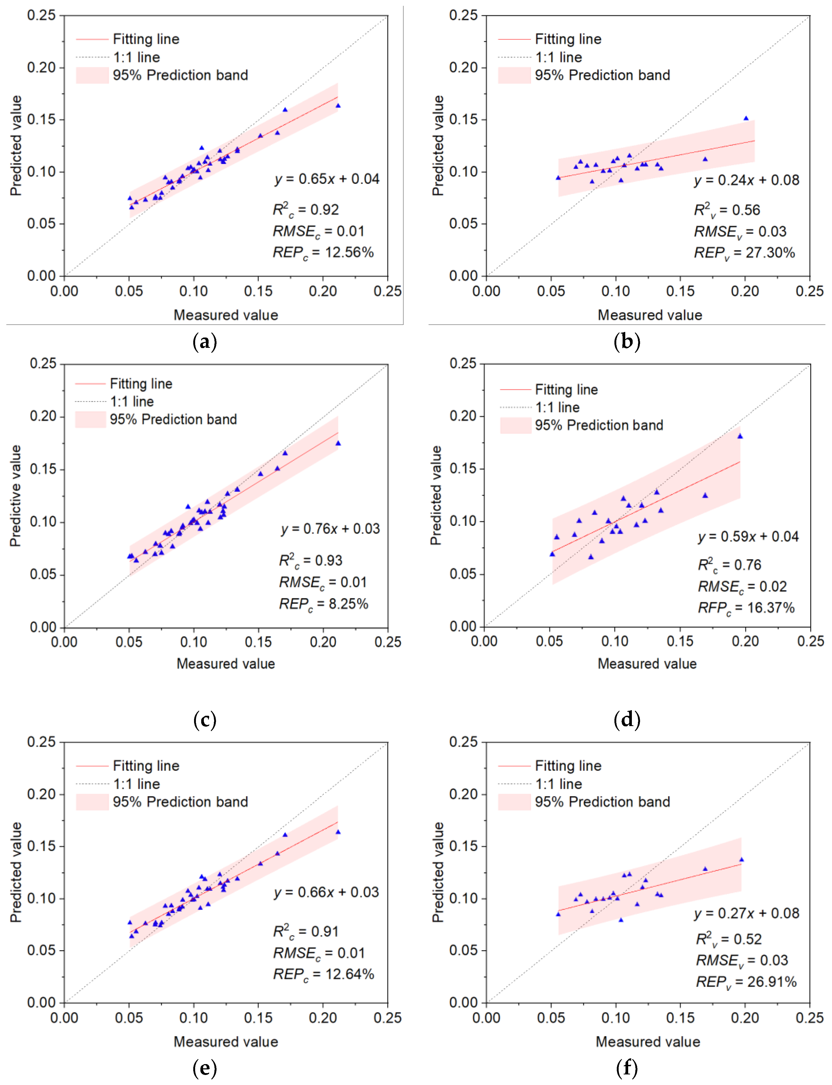
| RF | 16 | 0.92 | 0.01 | 12.64 | 0.56 | 0.03 | 27.30 | |
| FD + UAV | MSR | 23 | 0.83 | 0.01 | 11.02 | 0.65 | 0.02 | 21.48 |
| PLS | 21 | 0.75 | 0.01 | 16.56 | 0.71 | 0.02 | 17.65 | |
| BPNN | - | 0.85 | 0.01 | 11.48 | 0.69 | 0.02 | 19.43 | |
| RF | 17 | 0.93 | 0.01 | 8.25 | 0.76 | 0.02 | 16.37 | |
| CR + UAV | MSR | 24 | 0.87 | 0.01 | 11.57 | 0.35 | 0.03 | 28.99 |
| PLS | 25 | 0.61 | 0.03 | 31.58 | 0.37 | 0.03 | 31.59 | |
| BPNN | - | 0.73 | 0.02 | 17.44 | 0.56 | 0.03 | 24.48 | |
| RF | 15 | 0.91 | 0.01 | 12.64 | 0.52 | 0.03 | 26.91 | |
Publisher’s Note: MDPI stays neutral with regard to jurisdictional claims in published maps and institutional affiliations. |
© 2022 by the authors. Licensee MDPI, Basel, Switzerland. This article is an open access article distributed under the terms and conditions of the Creative Commons Attribution (CC BY) license (https://creativecommons.org/licenses/by/4.0/).
Share and Cite
Luo, L.; Chang, Q.; Gao, Y.; Jiang, D.; Li, F. Combining Different Transformations of Ground Hyperspectral Data with Unmanned Aerial Vehicle (UAV) Images for Anthocyanin Estimation in Tree Peony Leaves. Remote Sens. 2022, 14, 2271. https://0-doi-org.brum.beds.ac.uk/10.3390/rs14092271
Luo L, Chang Q, Gao Y, Jiang D, Li F. Combining Different Transformations of Ground Hyperspectral Data with Unmanned Aerial Vehicle (UAV) Images for Anthocyanin Estimation in Tree Peony Leaves. Remote Sensing. 2022; 14(9):2271. https://0-doi-org.brum.beds.ac.uk/10.3390/rs14092271
Chicago/Turabian StyleLuo, Lili, Qinrui Chang, Yifan Gao, Danyao Jiang, and Fenling Li. 2022. "Combining Different Transformations of Ground Hyperspectral Data with Unmanned Aerial Vehicle (UAV) Images for Anthocyanin Estimation in Tree Peony Leaves" Remote Sensing 14, no. 9: 2271. https://0-doi-org.brum.beds.ac.uk/10.3390/rs14092271