Use of Soil Moisture Variability in Artificial Neural Network Retrieval of Soil Moisture

Abstract

Passive microwave remote sensing is one of the most promising techniques for soil moisture retrieval. However, the inversion of soil moisture from brightness temperature observations is not straightforward, as it is influenced by numerous factors such as surface roughness, vegetation cover, and soil texture. Moreover, the relationship between brightness temperature, soil moisture and the factors mentioned above is highly non-linear and ill-posed. Consequently, Artificial Neural Networks (ANNs) have been used to retrieve soil moisture from microwave data, but with limited success when dealing with data different to that from the training period. In this study, an ANN is tested for its ability to predict soil moisture at 1 km resolution on different dates following training at the same site for a specific date. A novel approach that utilizes information on the variability of soil moisture, in terms of its mean and standard deviation for a (sub) region of spatial dimension up to 40 km, is used to improve the current retrieval accuracy of the ANN method. A comparison between the ANN with and without the use of the variability information showed that this enhancement enables the ANN to achieve an average Root Mean Square Error (RMSE) of around 5.1% v/v when using the variability information, as compared to around 7.5% v/v without it. The accuracy of the soil moisture retrieval was further improved by the division of the target site into smaller regions down to 4 km in size, with the spatial variability of soil moisture calculated from within the smaller region used in the ANN. With the combination of an ANN architecture of a single hidden layer of 20 neurons and the dual-polarized brightness temperatures as input, the proposed use of variability and sub-region methodology achieves an average retrieval accuracy of 3.7% v/v. Although this accuracy is not the lowest as comparing to the research in this field, the main contribution is the ability of ANN in solving the problem of predicting “out-of-range” soil moisture values. However, the applicability of this method is highly dependent on the accuracy of the mean and standard deviation values within the sub-region, potentially limiting its routine application.

1. Introduction

Soil moisture controls several processes at or near the land surface. These processes include: the partitioning of rainfall into infiltration and run-off [1], the partitioning of available energy into latent and sensible heat [2], the drainage to ground water and/or surface water [3], as well as the growth of vegetation [4]. All these processes are highly nonlinear functions of soil moisture [5], and so accurate soil moisture observations are crucial in order to forecast and predict these processes accurately.

Various approaches have been developed over the past two decades to infer near-surface soil moisture from remotely sensed measurements of surface temperature, radar backscatter, and microwave brightness temperature [6]. Among these, microwave radiometry has been the most successful of the remote sensing approaches for soil moisture estimation [7,8], due to its ability to penetrate cloud, its direct relationship with soil moisture through the soil’s dielectric constant, and a reduced sensitivity to land surface roughness and vegetation cover [9,10,11,12]. Consequently, the Soil Moisture and Ocean Salinity (SMOS) mission [13] launched in November 2009 is the first soil moisture dedicated satellite, using a 1.4 GHz 2-D interferometric polar orbiting L-band passive microwave sensor. This satellite will provide data on the 0-5 cm deep soil moisture content with a repeat cycle ranging from one to three days depending on latitude and the expected soil moisture accuracy of 4% v/v. Soil moisture retrieval will be from the L-band Microwave Emission of the Biosphere (L-MEB) model that simulates the microwave emission from a soil-vegetation layer [14]. L-MEB requires a great deal of ancillary information, including vegetation and surface type dependent parameters such as the vegetation opacity, vegetation scattering albedo and roughness, making the global application of this method difficult. While generic parameters have been published for a variety of land cover types [11], they have not been widely tested [14].

To overcome this difficulty, researchers in soil moisture problems have utilized data driven approaches. Artificial Neural Networks (ANNs) are one of the possible alternate approaches that have been used for soil moisture retrieval [15]. Specific examples include the work of Liou et al. [16] and Liu et al. [7], who used an Error Propagation Learning Backpropagation (EPLBP) to retrieve soil moisture (SM) from 1.4 GHz, 6.9 GHz and 10.65 GHz brightness temperature observations. Liou et al. [16] used simulated data from the Land Surface Process/Radiobrightness (LSP/R) model during a two-month dry-down of a prairie grassland having vegetation wet biomass of 3.7 km/m² [17], with 5% of 8,640 simulated Tb-SM pairs randomly chosen to train the ELPBP. Another 5% of the data were randomly chosen for testing. Experiments were then conducted for different combinations of brightness temperature (Tb) frequencies with different viewing angles. The retrieval result was a Root Mean Square Error (RMSE) of less than 1% v/v for all cases tested, and a correlation coefficient of better than 0.9. Conversely, Liu et al. [7] used Tb data obtained by the PORTOS radiometer over a wheat field during its three months growth cycle in 1993 (PORTOS-93) and 1996 (PORTOS-96). The EPLBP was trained with a subset of data from PORTOS-93 and tested on: (i) the remaining subset of PORTOS-93, and (ii) data from PORTOS-96. For both test cases, nearly half of the testing data were used for the validation of the EPLBP. The number of data used for training and testing were less than 10 points for each test case. From their research, the RMSE of retrieval achieved was about 5% v/v for all cases in 1993 and about 4% v/v in 1996. Although the retrieval result was encouraging, providing some confidence for the use of ANN for soil moisture retrieval, the small number of data used for training and testing was questionable. Moreover, the characteristics of the training and testing data in terms of its statistical centrality were not presented and if the data used for testing is similar to the training data, or the testing data is a subset of the training data, it is expected that the ANN would produce overly optimistic results.

For the case of using field data, the potential of ANN application within the context of ESA’s SMOS mission [18] over land has been studied by Angiuli et al. [19]. The standard backpropagation algorithm was trained with simulated data of the land emission model and tested with field data, using L-band radiometric observations of bare soils obtained during two field experiments: T-REX and MOUSE. A total of 2,000 data were simulated with 1,400 used for training and 600 for testing. The input vectors included Tb at different incidence angles, surface temperature and surface roughness, while the output vector was the soil moisture value. It was reported that the maximum RMSE was 7% v/v with the best RMSE obtained being 5% v/v, when applied to the data from one field experiment. For the other field experiment data, it was reported that the ANN tended to underestimate the soil moisture for water content larger than 15%, due to the fact that the ANN was trained using simulation data that in large percentage corresponded to water contents lower than this value. The ANN managed to obtain a RMSE of 4% v/v for soil moisture values lower than 15%. Moreover, the most current research by Lakhankar et al. [20] using active microwave data showed that when the “trained” ANN is tested on the same study areas but for a different date, the RMSE obtained was around 7–8% v/v, with RMSE being 4.4% v/v when it is tested with an independent hold-out sample on the same date and 3.6% v/v on the hold-out sample from the training data. This is a typical problem of ANN models which could not generalized for “out-of-range” data. However, it is crucial to solve this problem in order for ANN to be applicable to soil moisture retrieval. Clearly, the normal approach of ANN for soil moisture mapping fails to capture the natural variability of land surface conditions, leading to unacceptable results in soil moisture retrieval when applied to field data.

Consequently, this paper presents a novel ANN methodology that makes it applicable to a wider range of conditions to those used for training. The methodology utilizes the variability of soil moisture in terms of the mean and standard deviation to capture the land surface variability, and is demonstrated for soil moisture retrieval at 1 km spatial resolution using single incidence angle dual polarized passive microwave data at 1 km resolution. When applied to a study area of 40 km × 40 km, the retrieval process is done over smaller regions (termed “sub-grid” hereafter) to capture the spatial variability. The main assumption is that the variability between adjacent 1 km pixels is more similar than for pixels that are further apart. The mean and standard deviation values are calculated based on the 1 km data which falls inside the predetermined sub-grid size. The results show that using a combination of spatial statistics and sub-region division, the ANN can predict soil moisture evolution over time to a suitable accuracy (less than or equal to 4% v/v, corresponding to that expected from the SMOS mission, termed as “target error” in this paper).

While the requirement for information on the mean and standard deviation of soil moisture at coarse scales is a limitation of the method, one application of this approach may be in soil moisture downscaling. The mean and standard deviation values at a resolution coarser than the desired downscaled resolution can be retrieved from radar or optical sensors and this proposed methodology can then be incorporated with passive microwave data for downscaling purpose.

2. Study Area and Data Sets

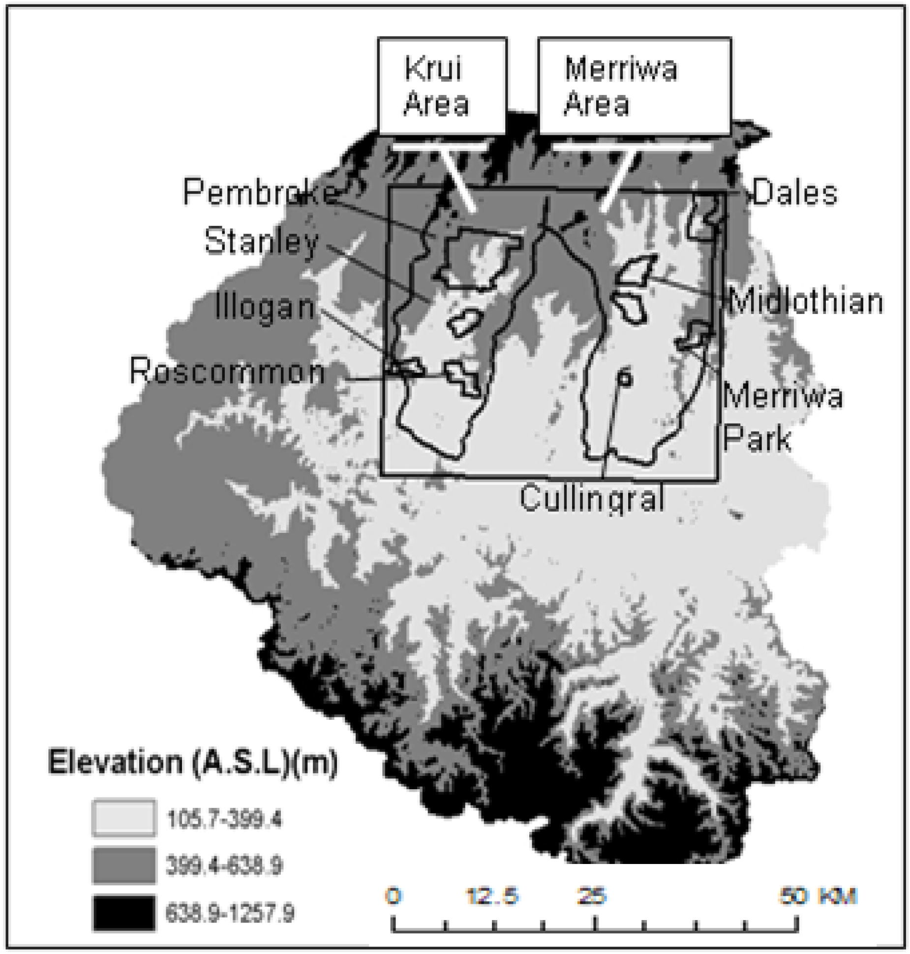
The study area is situated in the northern part of the Goulburn River catchment, located in a semiarid area of south-eastern Australia. This catchment extends from 31°46’S to 32°51’S and 149°40’E to 150°36’E with elevations ranging from 106 m in the floodplains to 1,257 m in the northern and southern mountain ranges (Figure 1). The area monitored during NAFE’05 was an area of approximately 40 km × 40 km, centered in the northern part of the catchment. Much of the original vegetation has been cleared to the north of the Goulburn River, where the dominant land uses are grazing and cropping. The southern part of the catchment is largely uncleared with extensive areas covered by eucalypt forest. Consequently the study area was chosen for its moderate-to-low vegetation cover condition. The area was logistically divided into two sub-areas, the “Merriwa” area in the east and the “Krui” area in the west.

Figure 1. Overview of NAFE’05 focus farms within the Krui and Merriwa areas.

Figure 1. Overview of NAFE’05 focus farms within the Krui and Merriwa areas.

The brightness temperature observations used in this study have been collected during the month-long NAFE field campaign held in November 2005. The campaign included extensive airborne passive microwave observations together with spatially distributed and in situ ground monitoring of soil moisture. For the purpose of this analysis, only pertinent details of the data are presented. A more detailed description of the data can be found in [21].

2.1. Microwave Data

Flights were conducted between October 31 and November 25 2005 using a small aircraft from the Airborne Research Australia national facility carrying the Polarimetric L-band Multi-beam Radiometer (PLMR). The PLMR measured both H and V polarized brightness temperatures (Tb) using a single receiver with polarization switch at incidence angles of +/−7°, +/−21° and +/−38.5° across track.

For the purpose of this study, only the “regional” L-band microwave data is used, providing full coverage across the 40km area with ground resolution of 1 km, resulting in a total of 1600 data points across 4 dates. All flights conducted were centered on the 6 a.m. overpass time of SMOS, and therefore well replicate the SMOS mission of the soil moisture retrieval conditions [22]. Due to the rough terrain, the actual pixel size varied between approximately 860 and 1,070 m, due to flying at a constant altitude above the median elevation of the study area.

In order to effectively use the push-broom radiometer data for soil moisture mapping, it was first necessary to account for the effect of varying beam angles and for the effects of varying soil temperature during the acquisition through a normalization procedure. The soil temperature was corrected by using the daily average of the soil temperatures at the monitoring stations recorded during the regional observation window. Previous studies by [23,24,25] showed that the angle normalization procedures can be developed over mixed land covers, by assuming that the deviation between measurements at different beam positions is due to the Fresnel effect, and that for a given day the Fresnel effect for a particular beam is constant for the range of soil moisture and vegetation present. From the studies mentioned above, it is assumed that by using a daily average for all data in an area at a common angle, errors due to anomalies in a particular beam that are not present in the others (e.g., a small water body) would be minimized. With this assumption, the normalization is applied as follows: (i) the daily average Tb over land targets is computed for each beam, (ii) a correction factor is computed by taking the ratio between the averages of each beam to the average of the reference beam, (iii) all the data for each beam on each day are then corrected using:

$$T{b}_i^N=T{b}_i\times \left(\raisebox{1ex}{$\overline{T{b}_i}$}\!\left/ \!\raisebox{-1ex}{$\overline{T{b}_{ref}}$}\right.\right)$$

(1)

where Tb_i is the individual Tb acquisition to be normalized, $T{b}_i^N$ is the normalized value, and $\overline{T{b}_i}$ and $\overline{T{b}_{ref}}$ are the daily average Tb values of the beam to be normalized and the reference beam respectively.

The regional Tb observations were normalized to the incidence angle of the radiometer outermost beams (±38.5°) using the procedure described above. This choice of angle was motivated by the fact that at close-to-nadir incidence angles, H- and V-polarized Tb values are very similar, while at off nadir, the V-polarized Tb data at higher incidence angle is generally higher than the H-polarized values (the amount of difference varies depending on the land surface conditions). The polarization difference yields information on the polarizing effect of the vegetation canopy when using wider incidence angle [18]. After normalization the Tb data is gridded onto a reference grid with uniform 1 km resolution. By averaging several individual Tb acquisitions into one Tb value for each cell, anomalies in individual readings are eliminated and the signal noise is reduced.

2.2. Soil Moisture Data

The soil moisture data for the 40 km × 40 km study area at 1 km nominal resolution was derived using the L-MEB model. A detailed description of this retrieval can be obtained from [22]. For the purpose of this paper, only pertinent details from [22] are presented.

The soil moisture maps derived from the 1 km airborne data have two major advantages with respect to ground point measurements: (i) they have a larger extent, covering the entire study area and therefore characterize the soil moisture variability within all the coarse-scale pixels, and (ii) each soil moisture observation represents an integrated value over a 1 km area, therefore overcoming the limitation of point data which only provides information for the domain sensed by a ground probe (a few centimeters).

The L-MEB model [26] is based on a simplified zero-order radiative transfer model, called the “tau-omega” approach [27]. The model takes into account the effect of a vegetation cover on soil emission, using ancillary data on land cover, near surface soil moisture and canopy temperature, and soil textural properties. For this study the ancillary data were obtained from either existing databases or derived from satellite imagery. In principle, ground collected data were given priority where possible. In the case where satellite imagery has been used, the dataset with the finest available resolution were chosen. This choice aims at minimizing any errors associated with the ancillary data so that the effects of land surface heterogeneity can be isolated. A summary of the ancillary data is shown in Table 1.

Table 1. Summary of the ancillary data used for the L-MEB model [22].

Ancillary Data	Source	Resolution	Description
Land cover	Landsat 5 Thermatic Mapper	30 m	Supervised classification and defined five land cover types: Native grass (50.7%) Dense forest (24.3%) Bare soil/vegetation with low Leaf Area Index (LAI) (12%) Open woodland (8.5%) Cropped area (4.5%)
Soil Texture	Ground sampling (Malvern Mastersizer 2000)	88 soil samples (7 cm wide, 5 cm deep) on two regional sampling days	Very variable, ranging from the black basalt derived cracking clays in the northern part to the sandstone derived soils in the southern part. An exact inverse distance technique was used to interpolate and upscale soil texture point data to the entire study area.
Soil Temperature	Monitoring stations	2.5 cm and 15 cm depth	Daily average obtained from the monitoring stations was used.
Canopy Temperature	Thermal infrared sensors	4 thermal infrared stations	Sensors were mounted on 2m high towers pointing vertically down towards the vegetation canopy of four different land covers: bare soil, lucerne crop, wheat crop and native grass.

Table 1. Summary of the ancillary data used for the L-MEB model [22].

Ancillary Data	Source	Resolution	Description
Land cover	Landsat 5 Thermatic Mapper	30 m	Supervised classification and defined five land cover types: Native grass (50.7%) Dense forest (24.3%) Bare soil/vegetation with low Leaf Area Index (LAI) (12%) Open woodland (8.5%) Cropped area (4.5%)
Soil Texture	Ground sampling (Malvern Mastersizer 2000)	88 soil samples (7 cm wide, 5 cm deep) on two regional sampling days	Very variable, ranging from the black basalt derived cracking clays in the northern part to the sandstone derived soils in the southern part. An exact inverse distance technique was used to interpolate and upscale soil texture point data to the entire study area.
Soil Temperature	Monitoring stations	2.5 cm and 15 cm depth	Daily average obtained from the monitoring stations was used.
Canopy Temperature	Thermal infrared sensors	4 thermal infrared stations	Sensors were mounted on 2m high towers pointing vertically down towards the vegetation canopy of four different land covers: bare soil, lucerne crop, wheat crop and native grass.

Soil moisture was retrieved by [22] for each cell of the 1 km Tb grid using the L-MEB model together with the ancillary data described in Table 1. The soil moisture output of the L-MEB model was limited to a maximum soil moisture value of 58% v/v, derived from the analysis of the maximum soil moisture achieved at the monitoring stations. Conversely, no lower limit was imposed on the retrieved soil moisture. The average accuracy of soil moisture retrieval at 1 km resolution using L-MEB was 3.8% v/v and in all cases better than 6% v/v over a variety of land surface conditions in the study area [22].

3. Methodology

3.1. Training, Validation, Testing and Verification Data

To find the optimum neural network architecture, the data was divided into: training, validation and testing sets through random sampling. The fully trained ANN is evaluated using the testing set. At this stage, the “trained” ANN is considered to be able to obtain an acceptable error when it is used for other similar situations. To verify that the “trained” ANN is able to maintain a similar result, “verification sets” are used.

The regional data measured on the 31 October 2005, 7 November 2005, 14 November 2005 and 21 November 2005 was the target dataset. As MODIS scenes were available for only three of the four days during NAFE’05, only data on 7, 14 and 21 November 2005 will be considered and discussed in this study. Data was binned into a 1 km reference grid for the whole 40 km $\times$40 km area. On occasions of missing data, i.e., the data from MODIS are not totally cloud free, the Inverse Distance Weighted (IDW) scheme was used to interpolate the values based on the surrounding values. As a result, a total of 1,600 data were obtained for each date. The data on 7 November 2005 were divided into training, validation and testing sets while data of 14 and 21 November 2005 were used for verification purpose.

3.2. Training Algorithm

In earlier work [28], a comparison of different training algorithms of Backpropagation Neural Network was undertaken using data from the same field experiment. It was found that the Broyden-Fletcher-Goldfarb-Shanno (BFGS) optimization method derived from the Newton method obtained the best retrieval results when different training algorithms were trained and tested with the same data set. For this reason, the BFGS method has been chosen for this study. The details of the neural network parameters used are given in Table 2.

Table 2. The training parameters for the BFGS training algorithm.

Performance goal	0.001
Maximum number of epochs to train	200
Minimum performance gradient	1e–10,000
Maximum validation failures	5
Name of line search routine to use	1-D minimization using Charalambous' method

Table 2. The training parameters for the BFGS training algorithm.

Performance goal	0.001
Maximum number of epochs to train	200
Minimum performance gradient	1e–10,000
Maximum validation failures	5
Name of line search routine to use	1-D minimization using Charalambous' method

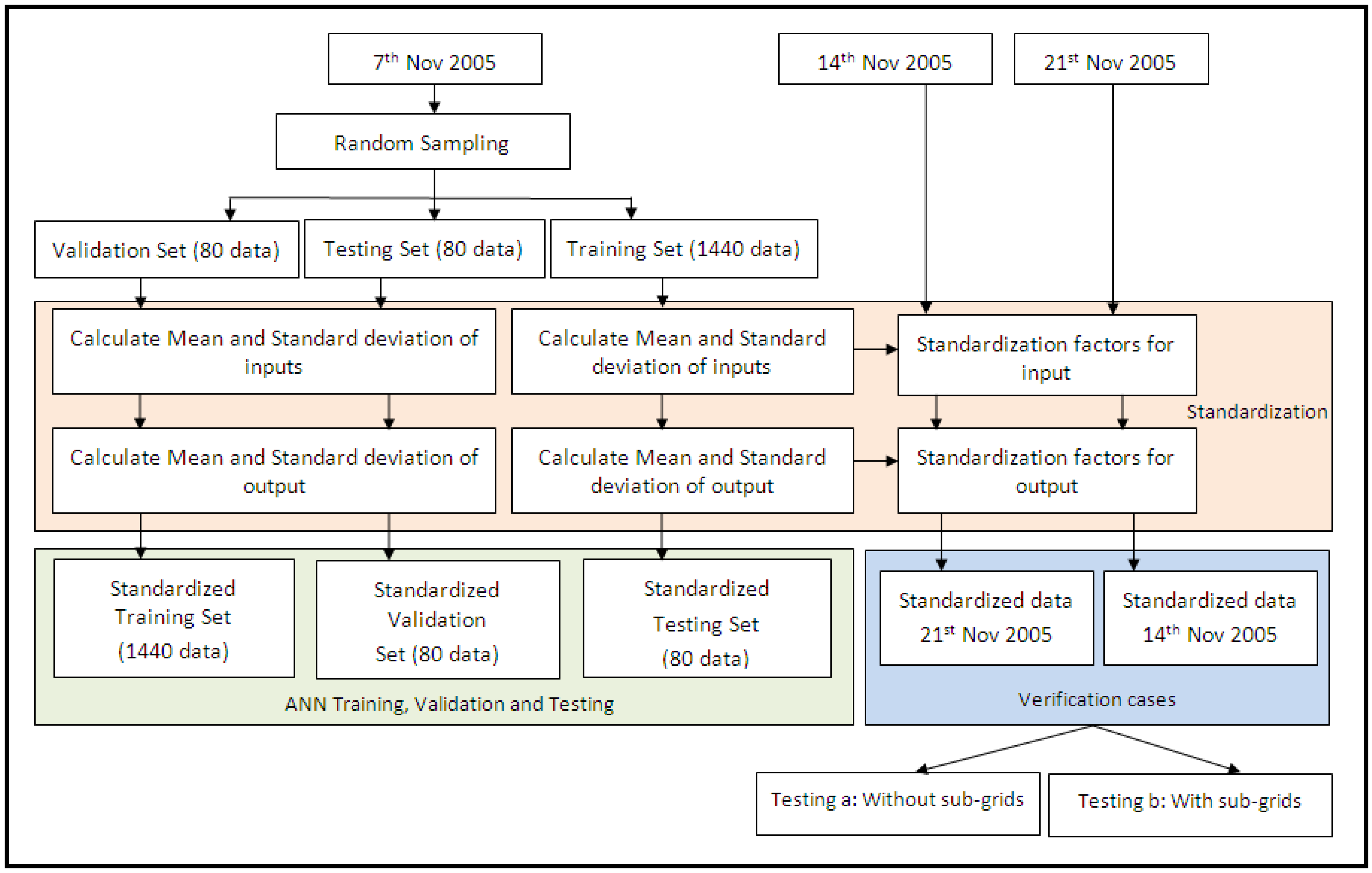
3.3. Pre- and Post-Processing Data for ANN: Standardization

The preprocessing aims to transform the data into a better form for the network to use [29]. This process, normally known as normalization or standardization, speeds up the training process of the ANN and reduces the likelihood of the ANN getting stuck in local minima. The normalization is mainly used to transform the input features to the same range of values in order to minimize the bias within the ANNs for one feature over another [30]. The training time is reduced by starting the training process for each feature within the same scale. This process is especially useful when the inputs of an application are on widely different scales. 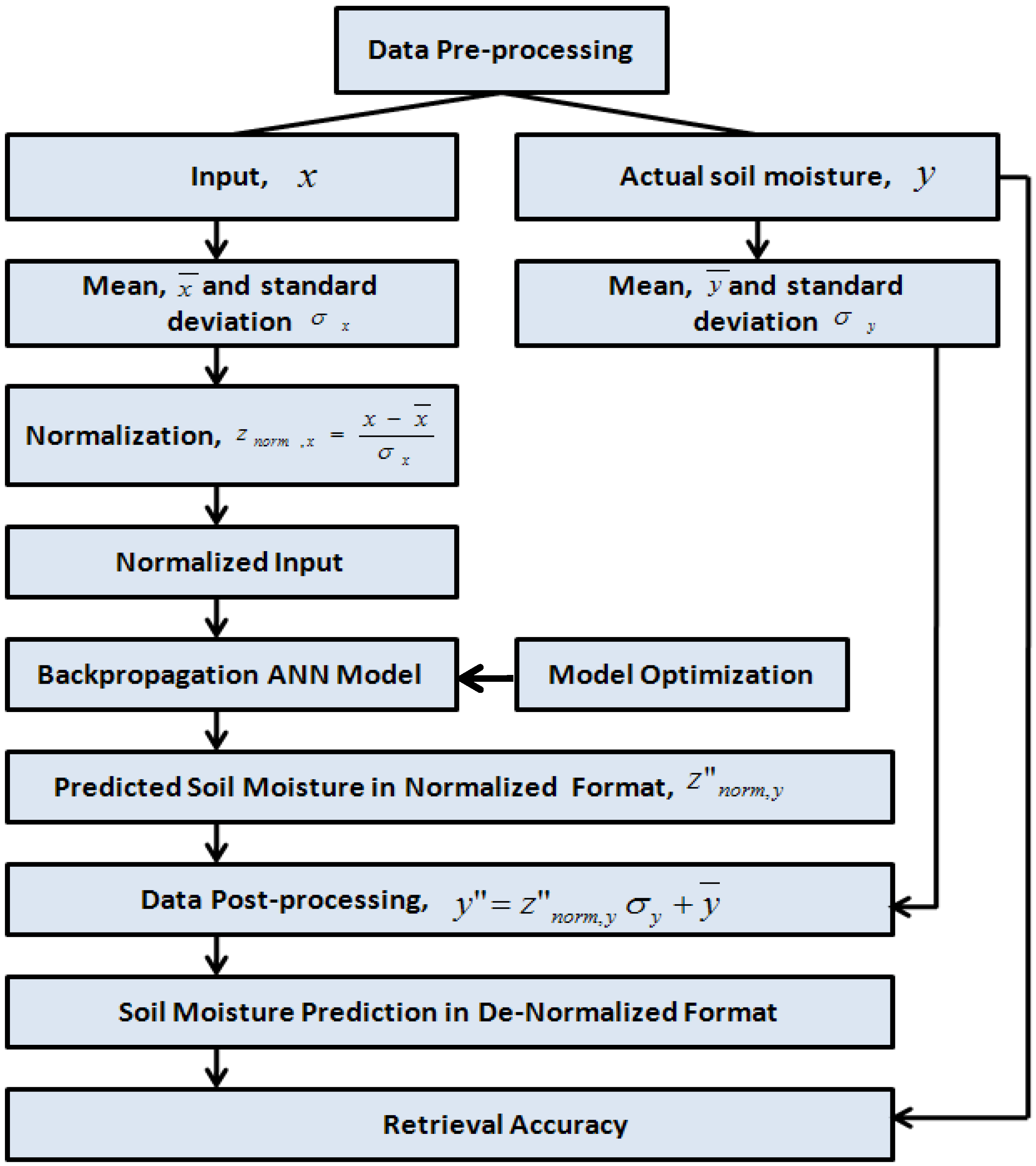One advantage of using the statistical normalization is to reduce the effects of outliers in the data [30]. There are different ways to normalize the data, and one of these is the statistical or Z-score normalization technique, which uses the mean and standard deviation for each feature across a set of training data to normalize each input feature vector. The input data will be normalized so that they have zero mean and unity standard deviation using:x

$$z_{norm}=\left(x-\overline{x}\right)\times \left(\frac{{\sigma }_y}{{\sigma }_x}\right)+\overline{y}$$

(2)

where z_norm is the normalized data, x is the input, $\overline{x}$ is the mean and σ_x is the standard deviation of the input data, the mean output, $\overline{y}$ is equal to 0, and the standard deviation of the output, σ_y is equal to 1. Equation 2 can be simplified and written as:

$$z_{norm}=\frac{x-\overline{x}}{{\sigma }_x}$$

(3)

Using Equation 3, the input data is transformed into normalized data. Besides obtaining the mean and standard deviation of the input of the training data, these statistical values are also obtained for the target of the training data in order to normalize the target data. The data are normalized before the training is commenced. All values leaving the ANNs will be in the standardized format. These values must subsequently be “destandardized” to provide meaningful results. This can be achieved by reversing the standardization algorithm used on the input modes [31]. The de-normalization of the normalized soil moisture is calculated based on Equation 4:

$$y″={z^{″}}_{norm,y}{\sigma }_y+\overline{y}$$

(4)

where y" is the de-normalized soil moisture values, z"_norm,y is the predicted soil moisture values in normalized format, σ_y and y is the standard deviation of mean of the soil moisture.

Figure 2 shows the process for the normalized and de-normalized process to pre- and post-processing the data.

Figure 2. The pre- and post-processing of the data.

Figure 2. The pre- and post-processing of the data.

The usual way of data preprocessing for ANNs is to obtain the standard deviation and mean from the training data [32]. Once the means and standard deviations are computed for each feature over the set of training data, they must be retained for use as weights in the final system design [30], otherwise the performance of the ANN will vary significantly if the ANN is trained using a different data representation than the unnormalized data. The study by Minns and Hall [33] points out the importance of standardizing data, particularly when the ANN fails to extrapolate correctly to out-of-range values. Their research concluded that, in practice, the ANN can only be used in the recall mode with data that it has “seen” before. In their rainfall-runoff model, different standardization factors were applied to the training and verification cases. For the case where they applied the same standardization factor from the training data to the verification data, the result was notably poorer. The results obtained from their research emphasized the care required in choosing the standardization factors. Moreover, previous work by the author of this paper [34] has shown that the performance of the ANN can be improved if the ANN is presented with data having similar statistical mean and standard deviation values.

In this research, the statistical normalization steps are taken to preprocess the data. In contrast to the usual way of using only the mean and standard deviation of the training data, the mean and standard deviation of the soil moisture of the validation, testing and evaluation data are also calculated to normalize the data. The rationale behind this is:

(i) The training is done using data from a single date. The condition of wetness/dryness for each date will almost certainly differ from the training date. From the literature, electromagnetic models that require a lot of ancillary data are often used to cover the variety of conditions required for training of the ANN. However, the spatial and temporal variability captured using the mean and standard deviation of the testing data can help to avoid this.

(ii) Even within a square meter, the surface soil moisture variance can be as large as over a whole field [35]. Therefore, it is crucial to incorporate the variability information in the soil moisture retrieval problem. A statistical approach such as calculating the central tendency (mean or median) and variability (variance or standard deviation) have been used to deal with field-scale variability [36]. In this study, this information is incorporated by standardizing the output with the mean and standard deviation values.

Within the same date, the spatial difference in soil moisture within the 40 km × 40 km target area is large. This is mainly due to the fact that soil moisture is influenced by many factors, making the estimation of its value using remote sensing a challenge. Consequently, the retrieval process of the whole 40 km × 40 km area involves dividing it into smaller regions. The spatial difference of soil moisture within a smaller region is smaller compared to a larger area, so when the spatial area is smaller, the prediction of the soil moisture value is expected to be easier. Selection of the size of this smaller region is explained later in this paper. For the purpose of this research, the mean and standard deviation of the soil moisture which are used for the normalization purpose were calculated based on the soil moisture for the grids that fall within the predetermined smaller region.

3.4. Input Data Selection

Besides the dual polarized brightness temperature, other ancillary data that potentially affects soil moisture retrieval are also assessed. Such ancillary data include the Normalized Difference Vegetation Index (NDVI) and Land Surface Temperature (LST) from the Moderate Resolution Imaging Spectroradiometer (MODIS). NDVI data were calculated from Band 1 and Band 2 of MODIS/Aqua Surface Reflectance Daily L2G Global 250 m data while the LST values are obtained from the MODIS/Aqua Land Surface Temperature and Emissivity Daily L3 Global 1 km data. Both of these ancillary data are gridded to the same 1 km reference grid as used in the processing of the brightness temperature and soil moisture data. The sensitivity of the ANN towards the inputs is measured by the change of Root Mean Square Error (RMSE) when an input is added to the model. The ANN is initialized and trained repeatedly until the global error between the referenced and computed values is driven down to an acceptable level. The ANN is then tested using the testing data which were randomly selected from the training set.

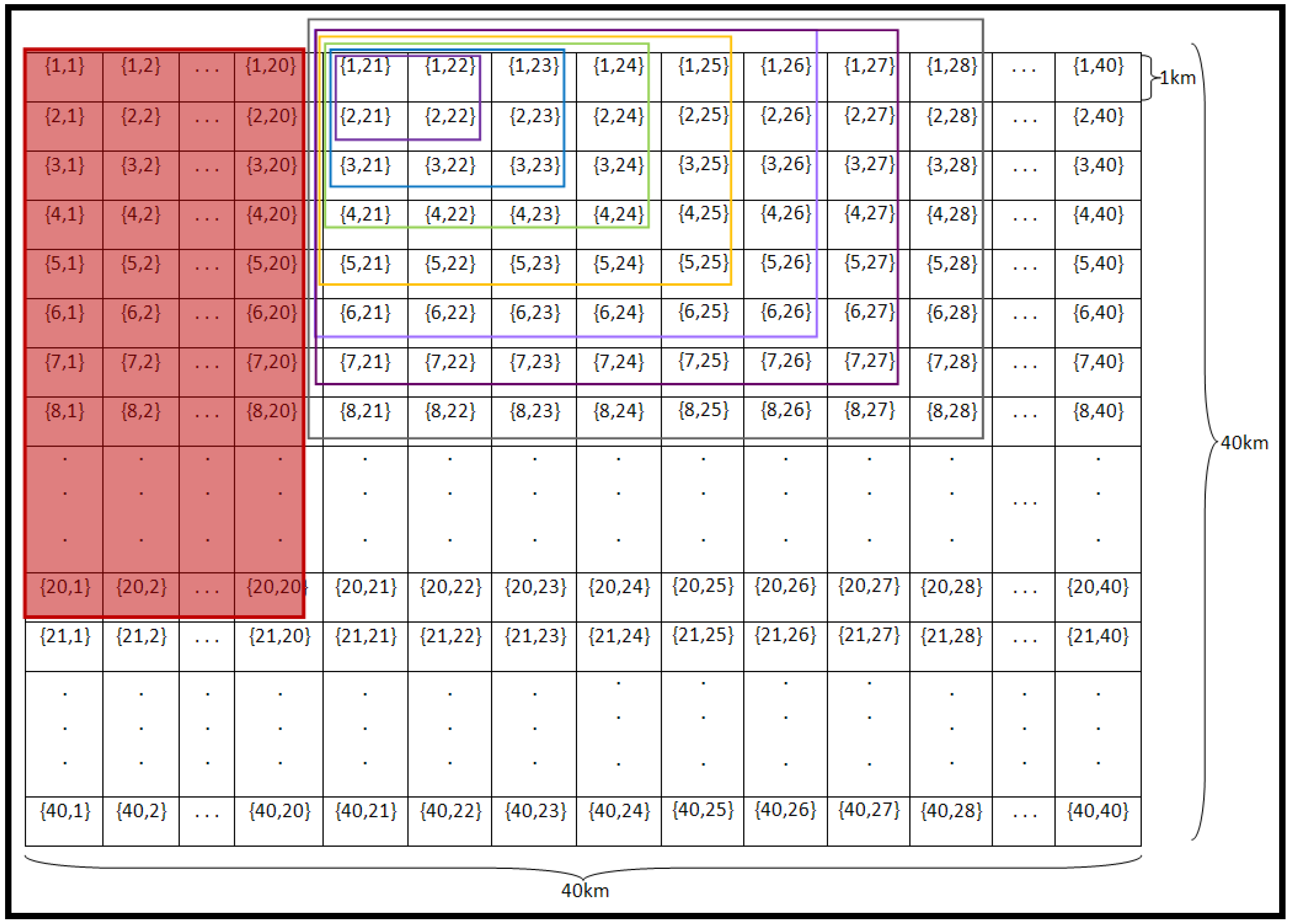
Figure 3. Sub-grid size and ANN determination using data on 7th November 2005. The red-filled data were used for training. The sub-grid sizes used are shown with unfilled boxes.

Figure 3. Sub-grid size and ANN determination using data on 7th November 2005. The red-filled data were used for training. The sub-grid sizes used are shown with unfilled boxes.

3.5. Selection of Sub-grid Size

The evaluation of the ANN was undertaken using data from two different dates, 14 and 21 November 2005, with the training data from 7 November 2005. Consequently, the land surface conditions for the evaluation dates were different from the training date. To account for both the spatial and temporal variability, the method of sub-region division was applied, and hence the optimum sub-region size needed to be determined. To avoid the use of any data from the 14 and 21 November 2005 before the verification process, the selection of sub-grid size and ANN architecture used data only from 7 November 2005. An area of size 20 km × 20 km in the north-west of the study area was arbitrary selected for this purpose. Among these 400 data, 5% (20 data) were randomly selected for each of the validation and testing. Training of the ANN was repeated until the ANN produced an acceptable accuracy. At this stage, the weights and biases of the ANN were retained. This ANN was next used for the selection of the different sub-grid sizes and ANN architecture. Sub-grid sizes of 2 km × 2 km, 3 km × 3 km, 4 km × 4 km, 5 km × 5 km, 6 km × 6 km, 7 km × 7 km and 8 km × 8 km were arbitrary selected from the north-east corner, with each sub-grid a sub-set of the next (Figure 3).

3.6. Neural Network Architecture

The number of input and output nodes is directly linked to the application. The different input combinations assessed include: (i) dual-polarized (H and V) brightness temperatures (TbH, TbV), (ii) TbH, TbV and NDVI, (iii) TbH, TbV and LST, and (iv) TbH, TbV with NDVI and LST. The output node is the soil moisture content.

Besides input and output layers, a decision needs to be made regarding the number of hidden layers and neurons. While ANNs with two hidden layers can represent functions of any shape [37], there is currently no theoretical reason to use neural networks with more than two hidden layers [38]. For this reason, the ANN architecture assessed here uses either one or two hidden layers; using too few or too many hidden neurons may undermine any application. Too few hidden neurons will cause under fitting whereby complicated signals within the data cannot be detected accurately by the ANN. On the other hand, using too many hidden neurons will cause over fitting whereby the neural network has so much information processing capacity that the limited amount of information contained in the training set is not enough to train all of the neurons in the hidden layers. Moreover, if too many hidden neurons are used, the length of training time will increase. The best way to optimize the number of hidden layers and hidden neurons is through trial and error method [39].

4. Results and Discussion

During the selection of the sub-grid size, the use of NDVI and LST as ancillary data for the soil moisture retrieval is also tested. Moreover, experiments were also conducted to determine the optimum ANN architecture. The results are summarized in terms of RMSE (% v/v) and correlation coefficient between the actual and predicted soil moisture values. To evaluate this methodology, the trained ANN was evaluated using the data from the 14 and 21 November 2005. Verification of the importance of combination of the both the standardization factor and the sub-grid method proposed in this paper is also presented. The dependency of the proposed method on the accuracy of the mean and standard deviation values are also shown.

4.1. Sub-grid Size and ANN Architecture

Table 3, Table 4, Table 5 and Table 6 show that the retrieval results deteriorate as the sub-grid size increases. For the purpose of sub-grid size selection, the optimum sub-grid size, i.e., the largest sub-grid size where the ANN can obtain the target error of 4% v/v is first identified. For the combination of TbH and TbV (Table 3), the optimum sub-grid size where the ANN can obtain an error of equal or less than 4% v/v (target error) is at 4 km × 4 km, with the number of hidden neurons being 20, 50 and 100 in the single and two hidden layers (equal number of hidden neurons in each layer). When the input consisted of TbH, TbV and NDVI (Table 4), with a single hidden layer of 20 neurons and two hidden layers of 10 hidden neurons in each layer (10:10), the ANN again achieved the target error at a sub-grid size of 4 km × 4 km. The same optimum sub-grid size was obtained for the case of TbH, TbV and LST (Table 5) and TbH, TbV, NDVI and LST (Table 6). As a result of this, the optimum sub-grid size is taken to be 4 km × 4 km.

Table 3. The impact on RMSE and R² for different numbers of hidden layers, hidden neurons and number of square grid subdivisions when using only TbH and TbV as input.

	Hidden neurons	RMSE (R2) Testing (%v/v)	RMSE (R2) for Different Verification Size (km) (% v/v)
			2 × 2	3 × 3	4 × 4	5 × 5	6 × 6	7 × 7	8 × 8
Single Layer	2	6.69 (0.34)	1.09 (0.77)	3.26 (0.49)	5.66 (0.54)	6.42 (0.42)	7.04 (0.63)	6.69 (0.31)	6.97 (0.38)
	4	6.45 (0.40)	1.14 (0.77)	3.12 (0.55)	5.35 (0.66)	6.07 (0.56)	6.73 (0.35)	6.38 (0.43)	6.71 (0.47)
	6	6.32 (0.34)	1.37 (0.91)	3.25 (0.30)	4.87 (0.56)	5.74 (0.46)	7.11 (0.20)	6.65 (0.26)	6.78 (0.32)
	8	6.34 (0.33)	1.42 (0.94)	3.75 (0.10)	5.31 (0.43)	5.75 (0.46)	6.89 (0.24)	6.52 (0.28)	6.83 (0.31)
	10	6.23 (0.37)	1.23 (0.63)	2.93 (0.56)	4.56 (0.69)	5.60 (0.49)	6.80 (0.26)	6.28 (0.34)	6.42 (0.41)
	20	5.75 (0.45)	1.42 (0.59)	2.44 (0.63)	2.86 (0.88)	4.52 (0.67)	5.75 (0.47)	5.27 (0.53)	5.53 (0.55)
	50	5.4 (0.54)	1.57 (0.62)	2.98 (0.46)	3.57 (0.75)	4.41 (0.68)	5.82 (0.46)	5.23 (0.54)	5.76 (0.51)
	100	5.39 (0.63)	1.44 (0.32)	3.21 (0.40)	3.08 (0.84)	4.51 (0.65)	5.22 (0.58)	4.66 (0.64)	5.21 (0.60)
Two Layers	2:2	7.01 (0.29)	1.05 (0.83)	3.70 (0.12)	6.24 (0.29)	6.82 (0.33)	7.33 (0.19)	7.05 (0.24)	7.38 (0.30)
	4:4	6.59 (0.31)	1.32 (0.91)	3.47 (0.23)	5.28 (0.53)	6.01 (0.46)	7.11 (0.20)	6.75 (0.24)	7.03 (0.29)
	5:5	6.42 (0.36)	1.13 (0.70)	3.52 (0.22)	5.60 (0.47)	6.19 (0.39)	6.95 (0.24)	6.56 (0.30)	6.74 (0.38)
	10:10	6.16 (0.37)	1.44 (0.91)	3.64 (0.13)	4.95 (0.55)	5.48 (0.53)	6.87 (0.25)	6.52 (0.28)	6.66 (0.35)
	20:20	5.86 (0.44)	1.44 (0.71)	2.72 (0.52)	3.63 (0.79)	4.61 (0.69)	5.81 (0.47)	5.57 (0.49)	5.92 (0.49)
	50:50	5.73 (0.47)	1.45 (0.74)	2.90 (0.49)	3.50 (0.78)	5.06 (0.56)	6.58 (0.34)	6.02 (0.41)	6.02 (0.47)
	100:100	5.74 (0.47)	1.50 (0.66)	3.16 (0.37)	3.25 (0.82)	3.93 (0.74)	4.68 (0.68)	4.12 (0.72)	5.16 (0.61)

Table 3. The impact on RMSE and R² for different numbers of hidden layers, hidden neurons and number of square grid subdivisions when using only TbH and TbV as input.

	Hidden neurons	RMSE (R2) Testing (%v/v)	RMSE (R2) for Different Verification Size (km) (% v/v)
			2 × 2	3 × 3	4 × 4	5 × 5	6 × 6	7 × 7	8 × 8
Single Layer	2	6.69 (0.34)	1.09 (0.77)	3.26 (0.49)	5.66 (0.54)	6.42 (0.42)	7.04 (0.63)	6.69 (0.31)	6.97 (0.38)
	4	6.45 (0.40)	1.14 (0.77)	3.12 (0.55)	5.35 (0.66)	6.07 (0.56)	6.73 (0.35)	6.38 (0.43)	6.71 (0.47)
	6	6.32 (0.34)	1.37 (0.91)	3.25 (0.30)	4.87 (0.56)	5.74 (0.46)	7.11 (0.20)	6.65 (0.26)	6.78 (0.32)
	8	6.34 (0.33)	1.42 (0.94)	3.75 (0.10)	5.31 (0.43)	5.75 (0.46)	6.89 (0.24)	6.52 (0.28)	6.83 (0.31)
	10	6.23 (0.37)	1.23 (0.63)	2.93 (0.56)	4.56 (0.69)	5.60 (0.49)	6.80 (0.26)	6.28 (0.34)	6.42 (0.41)
	20	5.75 (0.45)	1.42 (0.59)	2.44 (0.63)	2.86 (0.88)	4.52 (0.67)	5.75 (0.47)	5.27 (0.53)	5.53 (0.55)
	50	5.4 (0.54)	1.57 (0.62)	2.98 (0.46)	3.57 (0.75)	4.41 (0.68)	5.82 (0.46)	5.23 (0.54)	5.76 (0.51)
	100	5.39 (0.63)	1.44 (0.32)	3.21 (0.40)	3.08 (0.84)	4.51 (0.65)	5.22 (0.58)	4.66 (0.64)	5.21 (0.60)
Two Layers	2:2	7.01 (0.29)	1.05 (0.83)	3.70 (0.12)	6.24 (0.29)	6.82 (0.33)	7.33 (0.19)	7.05 (0.24)	7.38 (0.30)
	4:4	6.59 (0.31)	1.32 (0.91)	3.47 (0.23)	5.28 (0.53)	6.01 (0.46)	7.11 (0.20)	6.75 (0.24)	7.03 (0.29)
	5:5	6.42 (0.36)	1.13 (0.70)	3.52 (0.22)	5.60 (0.47)	6.19 (0.39)	6.95 (0.24)	6.56 (0.30)	6.74 (0.38)
	10:10	6.16 (0.37)	1.44 (0.91)	3.64 (0.13)	4.95 (0.55)	5.48 (0.53)	6.87 (0.25)	6.52 (0.28)	6.66 (0.35)
	20:20	5.86 (0.44)	1.44 (0.71)	2.72 (0.52)	3.63 (0.79)	4.61 (0.69)	5.81 (0.47)	5.57 (0.49)	5.92 (0.49)
	50:50	5.73 (0.47)	1.45 (0.74)	2.90 (0.49)	3.50 (0.78)	5.06 (0.56)	6.58 (0.34)	6.02 (0.41)	6.02 (0.47)
	100:100	5.74 (0.47)	1.50 (0.66)	3.16 (0.37)	3.25 (0.82)	3.93 (0.74)	4.68 (0.68)	4.12 (0.72)	5.16 (0.61)

Table 4. As for Table 3 but using TbH, TbV and NDVI as input.

	Hidden neurons	RMSE (R2) Testing (%v/v)	RMSE (R2) for Different Verification Size (km) (%v/v)
			2 × 2	3 × 3	4 × 4	5 × 5	6 × 6	7 × 7	8 × 8
Single Layer	2	6.30 (0.39)	1.29 (0.80)	2.84 (0.55)	4.58 (0.75)	5.78 (0.55)	6.75 (0.30)	6.37 (0.36)	6.64 (0.41)
	4	5.23 (0.63)	1.43 (0.91)	3.1 (0.36)	5.12 (0.46)	5.93 (0.41)	6.22 (0.40)	5.84 (0.45)	5.76 (0.54)
	6	5.34 (0.54)	1.55 (0.95)	3.09 (0.37)	4.53 (0.58)	5.33 (0.53)	6.23 (0.38)	5.84 (0.43)	5.89 (0.49)
	8	5.50 (0.50)	1.64 (0.88)	2.93 (0.43)	4.01 (0.69)	5.13 (0.58)	6.21 (0.40)	5.94 (0.41)	5.99 (0.48)
	10	5.56 (0.51)	1.41 (0.90)	3.04 (0.38)	4.89 (0.53)	5.50 (0.52)	5.41 (0.59)	5.09 (0.62)	5.19 (0.67)
	20	4.82 (0.64)	1.45 (0.71)	2.55 (0.58)	3.59 (0.80)	5.09 (0.58)	5.60 (0.51)	5.25 (0.55)	5.16 (0.63)
	50	5.46 (0.51)	1.60 (0.95)	3.36 (0.36)	4.49 (0.48)	5.92 (0.42)	6.11 (0.44)	5.57 (0.49)	5.46 (0.57)
	100	5.52 (0.49)	1.87 (1.00)	3.11 (0.49)	4.84 (0.52)	4.61 (0.64)	5.01 (0.61)	4.60 (0.65)	5.01 (0.64)
Two Layers	2:2	6.54 (0.39)	1.27 (0.89)	3.34 (0.31)	5.33 (0.63)	6.18 (0.53)	7.04 (0.26)	6.73 (0.30)	7.03 (0.36)
	4:4	5.84 (0.55)	1.32 (0.92)	3.11 (0.39)	5.12 (0.58)	5.86 (0.53)	6.17 (0.50)	5.91 (0.53)	6.12 (0.58)
	5:5	5.53 (0.56)	1.38 (0.86)	2.95 (0.44)	4.74 (0.62)	5.59 (0.52)	5.56 (0.57)	5.30 (0.61)	5.52 (0.65)
	10:10	5.57 (0.50)	1.55 (0.94)	2.60 (0.56)	3.96 (0.76)	5.15 (0.60)	6.46 (0.34)	6.12 (0.38)	6.22 (0.44)
	20:20	5.60 (0.51)	1.46 (0.22)	3.24 (0.31)	5.17 (0.44)	5.59 (0.48)	6.01 (0.43)	5.53 (0.50)	5.50 (0.58)
	50:50	5.27 (0.54)	1.46 (0.72)	2.85 (0.46)	5.27 (0.42)	5.42 (0.50)	5.91 (0.44)	5.44 (0.50)	5.43 (0.57)
	100:100	5.30 (0.54)	1.68 (1.00)	2.72 (0.61)	4.76 (0.53)	4.41 (0.76)	4.90 (0.70)	4.52 (0.71)	4.64 (0.72)

Table 4. As for Table 3 but using TbH, TbV and NDVI as input.

	Hidden neurons	RMSE (R2) Testing (%v/v)	RMSE (R2) for Different Verification Size (km) (%v/v)
			2 × 2	3 × 3	4 × 4	5 × 5	6 × 6	7 × 7	8 × 8
Single Layer	2	6.30 (0.39)	1.29 (0.80)	2.84 (0.55)	4.58 (0.75)	5.78 (0.55)	6.75 (0.30)	6.37 (0.36)	6.64 (0.41)
	4	5.23 (0.63)	1.43 (0.91)	3.1 (0.36)	5.12 (0.46)	5.93 (0.41)	6.22 (0.40)	5.84 (0.45)	5.76 (0.54)
	6	5.34 (0.54)	1.55 (0.95)	3.09 (0.37)	4.53 (0.58)	5.33 (0.53)	6.23 (0.38)	5.84 (0.43)	5.89 (0.49)
	8	5.50 (0.50)	1.64 (0.88)	2.93 (0.43)	4.01 (0.69)	5.13 (0.58)	6.21 (0.40)	5.94 (0.41)	5.99 (0.48)
	10	5.56 (0.51)	1.41 (0.90)	3.04 (0.38)	4.89 (0.53)	5.50 (0.52)	5.41 (0.59)	5.09 (0.62)	5.19 (0.67)
	20	4.82 (0.64)	1.45 (0.71)	2.55 (0.58)	3.59 (0.80)	5.09 (0.58)	5.60 (0.51)	5.25 (0.55)	5.16 (0.63)
	50	5.46 (0.51)	1.60 (0.95)	3.36 (0.36)	4.49 (0.48)	5.92 (0.42)	6.11 (0.44)	5.57 (0.49)	5.46 (0.57)
	100	5.52 (0.49)	1.87 (1.00)	3.11 (0.49)	4.84 (0.52)	4.61 (0.64)	5.01 (0.61)	4.60 (0.65)	5.01 (0.64)
Two Layers	2:2	6.54 (0.39)	1.27 (0.89)	3.34 (0.31)	5.33 (0.63)	6.18 (0.53)	7.04 (0.26)	6.73 (0.30)	7.03 (0.36)
	4:4	5.84 (0.55)	1.32 (0.92)	3.11 (0.39)	5.12 (0.58)	5.86 (0.53)	6.17 (0.50)	5.91 (0.53)	6.12 (0.58)
	5:5	5.53 (0.56)	1.38 (0.86)	2.95 (0.44)	4.74 (0.62)	5.59 (0.52)	5.56 (0.57)	5.30 (0.61)	5.52 (0.65)
	10:10	5.57 (0.50)	1.55 (0.94)	2.60 (0.56)	3.96 (0.76)	5.15 (0.60)	6.46 (0.34)	6.12 (0.38)	6.22 (0.44)
	20:20	5.60 (0.51)	1.46 (0.22)	3.24 (0.31)	5.17 (0.44)	5.59 (0.48)	6.01 (0.43)	5.53 (0.50)	5.50 (0.58)
	50:50	5.27 (0.54)	1.46 (0.72)	2.85 (0.46)	5.27 (0.42)	5.42 (0.50)	5.91 (0.44)	5.44 (0.50)	5.43 (0.57)
	100:100	5.30 (0.54)	1.68 (1.00)	2.72 (0.61)	4.76 (0.53)	4.41 (0.76)	4.90 (0.70)	4.52 (0.71)	4.64 (0.72)

Table 5. As for Table 3 but using TbH, TbV and LST as input.

	Hidden neurons	RMSE (R2) Testing (%v/v)	RMSE (R2) for Different Verification Size (km) (%v/v)
			2 × 2	3 × 3	4 × 4	5 × 5	6 × 6	7 × 7	8 × 8
Single Layer	2	6.51 (0.42)	1.11 (0.56)	2.88 (0.67)	5.22 (0.67)	6.34 (0.46)	7.09 (0.24)	6.54 (0.37)	6.76 (0.45)
	4	5.72 (0.46)	1.43 (0.76)	2.93 (0.43)	4.16 (0.65)	5.27 (0.55)	6.09 (0.42)	5.52 (0.50)	5.60 (0.55)
	6	5.98 (0.43)	1.33 (0.87)	3.20 (0.33)	4.66 (0.64)	5.21 (0.59)	6.04 (0.46)	5.66 (0.52)	5.82 (0.56)
	8	5.84 (0.50)	1.38 (0.94)	2.75 (0.50)	4.27 (0.64)	5.56 (0.48)	6.46 (0.33)	5.67 (0.46)	5.59 (0.55)
	10	5.66 (0.48)	1.36 (0.68)	2.56 (0.59)	3.59 (0.77)	5.36 (0.53)	5.93 (0.46)	5.25 (0.56)	5.25 (0.62)
	20	5.73 (0.47)	1.23 (0.68)	2.59 (0.62)	3.68 (0.76)	5.59 (0.47)	6.06 (0.41)	5.20 (0.56)	4.99 (0.66)
	50	5.27 (0.54)	1.33 (0.87)	2.31 (0.66)	3.62 (0.76)	5.30 (0.52)	6.39 (0.39)	5.65 (0.48)	5.55 (0.55)
	100	4.81 (0.62)	1.33 (0.46)	3.63 (0.32)	4.49 (0.60)	5.58 (0.49)	6.07 (0.42)	5.39 (0.51)	5.82 (0.51)
Two Layers	2:2	6.75 (0.39)	1.13 (0.63)	3.46 (0.25)	5.70 (0.48)	6.73 (0.46)	7.06 (0.29)	6.79 (0.31)	7.14 (0.34)
	4:4	5.85 (0.50)	1.17 (0.75)	2.64 (0.60)	3.95 (0.78)	5.28 (0.61)	5.85 (0.50)	5.31 (0.60)	5.38 (0.51)
	5:5	6.09 (0.50)	1.12 (0.72)	3.04 (0.50)	4.86 (0.72)	5.84 (0.62)	6.16 (0.53)	5.77 (0.61)	5.95 (0.68)
	10:10	5.93 (0.42)	1.46 (0.92)	2.82 (0.50)	3.92 (0.77)	5.52 (0.52)	6.69 (0.29)	6.01 (0.40)	6.07 (0.38)
	20:20	5.59 (0.48)	1.54 (0.91)	3.50 (0.21)	4.75 (0.53)	5.39 (0.51)	6.27 (0.37)	5.66 (0.46)	5.62 (0.55)
	50:50	5.56 (0.49)	1.46 (0.61)	2.49 (0.63)	2.79 (0.84)	4.56 (0.83)	5.29 (0.56)	4.70 (0.63)	4.84 (0.66)
	100:100	5.08 (0.57)	1.54 (0.39)	3.24 (0.34)	4.61 (0.56)	5.41 (0.50)	5.97 (0.44)	4.99 (0.60)	5.24 (0.62)

Table 5. As for Table 3 but using TbH, TbV and LST as input.

	Hidden neurons	RMSE (R2) Testing (%v/v)	RMSE (R2) for Different Verification Size (km) (%v/v)
			2 × 2	3 × 3	4 × 4	5 × 5	6 × 6	7 × 7	8 × 8
Single Layer	2	6.51 (0.42)	1.11 (0.56)	2.88 (0.67)	5.22 (0.67)	6.34 (0.46)	7.09 (0.24)	6.54 (0.37)	6.76 (0.45)
	4	5.72 (0.46)	1.43 (0.76)	2.93 (0.43)	4.16 (0.65)	5.27 (0.55)	6.09 (0.42)	5.52 (0.50)	5.60 (0.55)
	6	5.98 (0.43)	1.33 (0.87)	3.20 (0.33)	4.66 (0.64)	5.21 (0.59)	6.04 (0.46)	5.66 (0.52)	5.82 (0.56)
	8	5.84 (0.50)	1.38 (0.94)	2.75 (0.50)	4.27 (0.64)	5.56 (0.48)	6.46 (0.33)	5.67 (0.46)	5.59 (0.55)
	10	5.66 (0.48)	1.36 (0.68)	2.56 (0.59)	3.59 (0.77)	5.36 (0.53)	5.93 (0.46)	5.25 (0.56)	5.25 (0.62)
	20	5.73 (0.47)	1.23 (0.68)	2.59 (0.62)	3.68 (0.76)	5.59 (0.47)	6.06 (0.41)	5.20 (0.56)	4.99 (0.66)
	50	5.27 (0.54)	1.33 (0.87)	2.31 (0.66)	3.62 (0.76)	5.30 (0.52)	6.39 (0.39)	5.65 (0.48)	5.55 (0.55)
	100	4.81 (0.62)	1.33 (0.46)	3.63 (0.32)	4.49 (0.60)	5.58 (0.49)	6.07 (0.42)	5.39 (0.51)	5.82 (0.51)
Two Layers	2:2	6.75 (0.39)	1.13 (0.63)	3.46 (0.25)	5.70 (0.48)	6.73 (0.46)	7.06 (0.29)	6.79 (0.31)	7.14 (0.34)
	4:4	5.85 (0.50)	1.17 (0.75)	2.64 (0.60)	3.95 (0.78)	5.28 (0.61)	5.85 (0.50)	5.31 (0.60)	5.38 (0.51)
	5:5	6.09 (0.50)	1.12 (0.72)	3.04 (0.50)	4.86 (0.72)	5.84 (0.62)	6.16 (0.53)	5.77 (0.61)	5.95 (0.68)
	10:10	5.93 (0.42)	1.46 (0.92)	2.82 (0.50)	3.92 (0.77)	5.52 (0.52)	6.69 (0.29)	6.01 (0.40)	6.07 (0.38)
	20:20	5.59 (0.48)	1.54 (0.91)	3.50 (0.21)	4.75 (0.53)	5.39 (0.51)	6.27 (0.37)	5.66 (0.46)	5.62 (0.55)
	50:50	5.56 (0.49)	1.46 (0.61)	2.49 (0.63)	2.79 (0.84)	4.56 (0.83)	5.29 (0.56)	4.70 (0.63)	4.84 (0.66)
	100:100	5.08 (0.57)	1.54 (0.39)	3.24 (0.34)	4.61 (0.56)	5.41 (0.50)	5.97 (0.44)	4.99 (0.60)	5.24 (0.62)

Table 6. As for Table 3 but using TbH, TbV, NDVI and LST as input.

	Hidden neurons	RMSE(R2) testing (%v/v)	RMSE (R2) for Different Verification Size (km) (%v/v)
			2 × 2	3 × 3	4 × 4	5 × 5	6 × 6	7 × 7	8 × 8
Single Layer	2	6.45 (0.53)	1.13 (0.35)	3.25 (0.35)	5.86 (0.33)	7.03 (0.17)	7.29 (0.51)	6.71 (0.31)	6.78 (0.47)
	4	5.54 (0.50)	1.51 (0.92)	2.96 (0.41)	4.43 (0.63)	5.53 (0.50)	6.44 (0.34)	6.04 (0.39)	6.08 (0.47)
	6	5.69 (0.60)	1.27 (0.88)	2.81 (0.60)	4.69 (0.77)	5.68 (0.62)	6.34 (0.45)	5.96 (0.52)	6.11 (0.59)
	8	5.78 (0.50)	1.31 (0.91)	2.68 (0.57)	4.01 (0.80)	5.04 (0.71)	5.82 (0.54)	5.52 (0.59)	5.66 (0.63)
	10	5.79 (0.45)	1.41 (0.98)	3.18 (0.33)	4.83 (0.58)	5.71 (0.49)	6.49 (0.33)	6.00 (0.41)	6.03 (0.52)
	20	5.78 (0.46)	1.27 (0.66)	2.97 (0.43)	4.35 (0.68)	5.53 (0.53)	5.88 (0.49)	5.30 (0.58)	5.60 (0.59)
	50	4.96 (0.59)	1.59 (0.95)	3.41 (0.27)	5.21 (0.45)	6.06 (0.38)	6.52 (0.34)	6.05 (0.40)	5.78 (0.51)
	100	4.93 (0.61)	1.54 (0.22)	3.67 (0.22)	3.69 (0.72)	5.47 (0.50)	6.54 (0.35)	5.68 (0.48)	5.62 (0.54)
Two Layers	2:2	6.69 (0.48)	1.15 (0.89)	3.43 (0.31)	5.81 (0.55)	6.57 (0.50)	6.94 (0.45)	6.68 (0.48)	7.03 (0.53)
	4:4	6.04 (0.62)	1.22 (1.00)	3.42 (0.23)	6.06 (0.28)	6.79 (0.25)	7.13 (0.22)	6.66 (0.31)	6.76 (0.43)
	5:5	5.31 (0.60)	1.25 (0.74)	3.05 (0.41)	4.48 (0.67)	5.27 (0.62)	6.04 (0.47)	5.54 (0.54)	5.81 (0.58)
	10:10	5.53 (0.56)	1.30 (0.87)	3.09 (0.41)	4.49 (0.70)	5.24 (0.64)	6.05 (0.47)	5.69 (0.53)	5.81 (0.58)
	20:20	5.70 (0.47)	1.37 (0.61)	2.96 (0.43)	4.12 (0.44)	5.10 (0.59)	6.03 (0.43)	5.51 (0.51)	5.95 (0.49)
	50:50	5.48 (0.51)	1.51 (0.95)	3.23 (0.32)	4.10 (0.67)	5.07 (0.60)	6.00 (0.44)	5.66 (0.47)	5.80 (0.51)
	100:100	4.40 (0.68)	1.72 (0.77)	3.21 (0.34)	4.61 (0.55)	6.70 (0.29)	7.21 (0.24)	5.84 (0.44)	5.47 (0.56)

Table 6. As for Table 3 but using TbH, TbV, NDVI and LST as input.

	Hidden neurons	RMSE(R2) testing (%v/v)	RMSE (R2) for Different Verification Size (km) (%v/v)
			2 × 2	3 × 3	4 × 4	5 × 5	6 × 6	7 × 7	8 × 8
Single Layer	2	6.45 (0.53)	1.13 (0.35)	3.25 (0.35)	5.86 (0.33)	7.03 (0.17)	7.29 (0.51)	6.71 (0.31)	6.78 (0.47)
	4	5.54 (0.50)	1.51 (0.92)	2.96 (0.41)	4.43 (0.63)	5.53 (0.50)	6.44 (0.34)	6.04 (0.39)	6.08 (0.47)
	6	5.69 (0.60)	1.27 (0.88)	2.81 (0.60)	4.69 (0.77)	5.68 (0.62)	6.34 (0.45)	5.96 (0.52)	6.11 (0.59)
	8	5.78 (0.50)	1.31 (0.91)	2.68 (0.57)	4.01 (0.80)	5.04 (0.71)	5.82 (0.54)	5.52 (0.59)	5.66 (0.63)
	10	5.79 (0.45)	1.41 (0.98)	3.18 (0.33)	4.83 (0.58)	5.71 (0.49)	6.49 (0.33)	6.00 (0.41)	6.03 (0.52)
	20	5.78 (0.46)	1.27 (0.66)	2.97 (0.43)	4.35 (0.68)	5.53 (0.53)	5.88 (0.49)	5.30 (0.58)	5.60 (0.59)
	50	4.96 (0.59)	1.59 (0.95)	3.41 (0.27)	5.21 (0.45)	6.06 (0.38)	6.52 (0.34)	6.05 (0.40)	5.78 (0.51)
	100	4.93 (0.61)	1.54 (0.22)	3.67 (0.22)	3.69 (0.72)	5.47 (0.50)	6.54 (0.35)	5.68 (0.48)	5.62 (0.54)
Two Layers	2:2	6.69 (0.48)	1.15 (0.89)	3.43 (0.31)	5.81 (0.55)	6.57 (0.50)	6.94 (0.45)	6.68 (0.48)	7.03 (0.53)
	4:4	6.04 (0.62)	1.22 (1.00)	3.42 (0.23)	6.06 (0.28)	6.79 (0.25)	7.13 (0.22)	6.66 (0.31)	6.76 (0.43)
	5:5	5.31 (0.60)	1.25 (0.74)	3.05 (0.41)	4.48 (0.67)	5.27 (0.62)	6.04 (0.47)	5.54 (0.54)	5.81 (0.58)
	10:10	5.53 (0.56)	1.30 (0.87)	3.09 (0.41)	4.49 (0.70)	5.24 (0.64)	6.05 (0.47)	5.69 (0.53)	5.81 (0.58)
	20:20	5.70 (0.47)	1.37 (0.61)	2.96 (0.43)	4.12 (0.44)	5.10 (0.59)	6.03 (0.43)	5.51 (0.51)	5.95 (0.49)
	50:50	5.48 (0.51)	1.51 (0.95)	3.23 (0.32)	4.10 (0.67)	5.07 (0.60)	6.00 (0.44)	5.66 (0.47)	5.80 (0.51)
	100:100	4.40 (0.68)	1.72 (0.77)	3.21 (0.34)	4.61 (0.55)	6.70 (0.29)	7.21 (0.24)	5.84 (0.44)	5.47 (0.56)

The optimal number of inputs, hidden layers, and neurons was selected from the column of 4 km × 4 km sub-grid size. The lowest RMSE obtained at the sub-grid size of 4 km × 4 km is 2.79% v/v (R² = 0.84) with two hidden layers of 50 neurons in each layer when TbH, TbV and LST were used as the input (Table 5). For the same sub-grid size, the use of only TbH and TbV as input managed to obtain a RMSE of 2.86% v/v (R² = 0.88) using single hidden layer of 20 neurons. Although this RMSE is slightly higher than when LST was included, fewer resources are needed. Moreover, according to Vonk et al. [40] simple neural networks are preferred over complex ones, provided they exhibit similar performances. Therefore a single hidden layer of 20 hidden neurons is preferred compared to two hidden layers of 50 neurons in each layer. 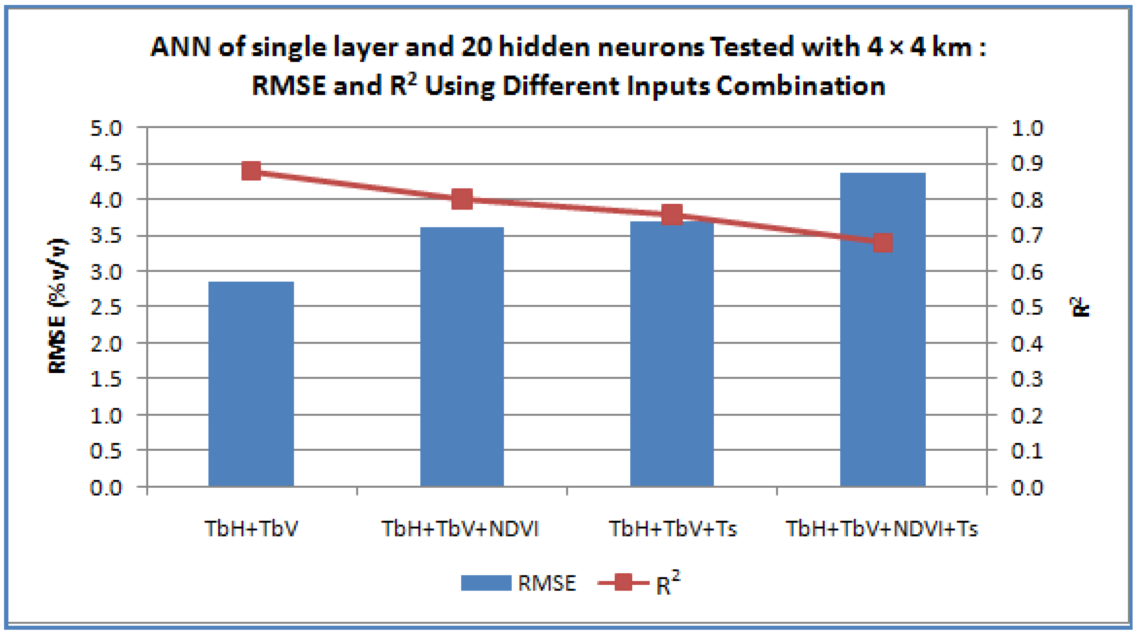Figure 4 shows the graph of RMSE and R² obtained when different combinations of inputs were used with this architecture. From this graph, it is clearly seen that the use of TbH and TbV promises the lowest RMSE value. Therefore the ANN architecture chosen was two inputs (TbH and TbV), a single hidden layer of 20 neurons, and 1 output.

4.2. Testing and Evaluation

Using the determined optimal ANN architecture (two inputs, one hidden layer of 20 neurons and one output), training was undertaken using data from the 7 November 2005. From the 1,600 data of the 7 November 2005, 1,440 data (90%) were randomly selected for training, with the remaining data divided equally (80 data or 5%) for the validation and testing of the ANN. The ANN was then trained to minimize the RMSE between the referenced and retrieved soil moisture values. At this stage, the weights and bias of the ANN, termed as “trained ANN”, were stored for verification using all the data of 14 and 21 November 2005. For each of the verification dates, the retrieval was carried out for each of the 1 km cells within the 4km×4km sub-grid from top-left corner to the right and then down until the lower-right corner of the target area. The statistical mean and standard deviation for each of the 4km×4km sub-grids were calculated to standardize and de-standardize the data.

The statistical mean and standard deviation for each date are given in Table 7, showing that the training data from the 7 November 2005 is wetter compared to the verification cases of the 14 and 21 November 2005. This shows that the spatial condition of the training data is different from the data used for the evaluation cases. Figure 4 shows clearly show that, at the sub-grid size of 4 km × 4 km, the use of ANN with TbH and TbV as the input managed to produce the lowest RMSE and highest R² with TbH and TbV as the combination inputs.

Figure 4. The results obtained for the 4 km × 4 km sub-grid when using the trained ANN of pre-determined ANN architecture with different input combinations.

Figure 4. The results obtained for the 4 km × 4 km sub-grid when using the trained ANN of pre-determined ANN architecture with different input combinations.

Table 7. Statistical means and standard deviations for the dual polarized brightness temperature and soil moisture values for training (7 November) and verification (14 November and 21 November).

Date	TbH (K)		TbV (K)		Soil Moisture (v/v)
	Mean	Standard deviation	Mean	Standard deviation	Mean	Standard deviation
7 November 05	241.5	10.1	261.4	7.8	0.39	0.12
14 November 05	266.0	6.5	279.3	5.4	0.18	0.10
21 November 05	271.3	3.9	282.6	3.1	0.16	0.08

Table 7. Statistical means and standard deviations for the dual polarized brightness temperature and soil moisture values for training (7 November) and verification (14 November and 21 November).

Date	TbH (K)		TbV (K)		Soil Moisture (v/v)
	Mean	Standard deviation	Mean	Standard deviation	Mean	Standard deviation
7 November 05	241.5	10.1	261.4	7.8	0.39	0.12
14 November 05	266.0	6.5	279.3	5.4	0.18	0.10
21 November 05	271.3	3.9	282.6	3.1	0.16	0.08

For the evaluation phase, the target area of 40 km × 40 km is divided into sub-grids of 4 km × 4 km. In other words, the retrieval using the trained ANN is not done for the entire 40 km × 40 km at once, but rather, the retrieval process is divided into 4 km × 4 km sub-grids. The soil moisture values at 1 km resolution are retrieved during each retrieval step at the sub-grids. This process is similar to a “window” that starts from the north-west corner of the target area, moving to the right and down.

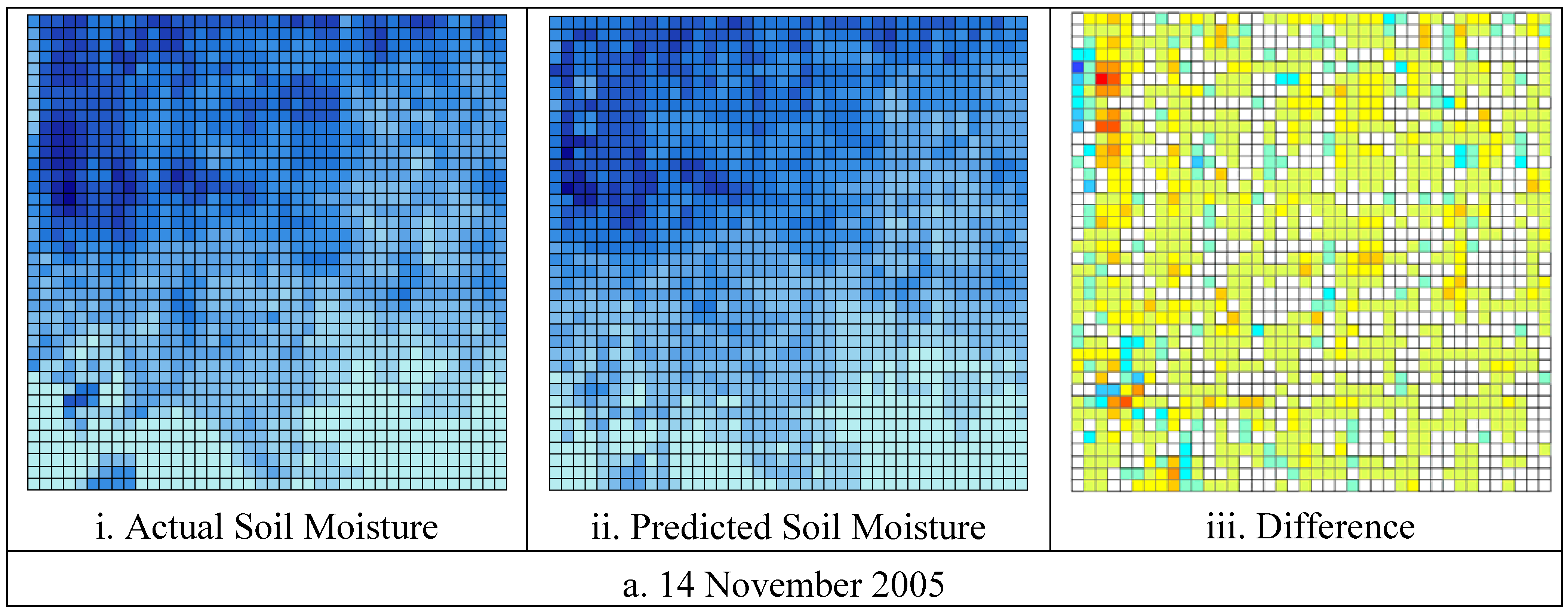
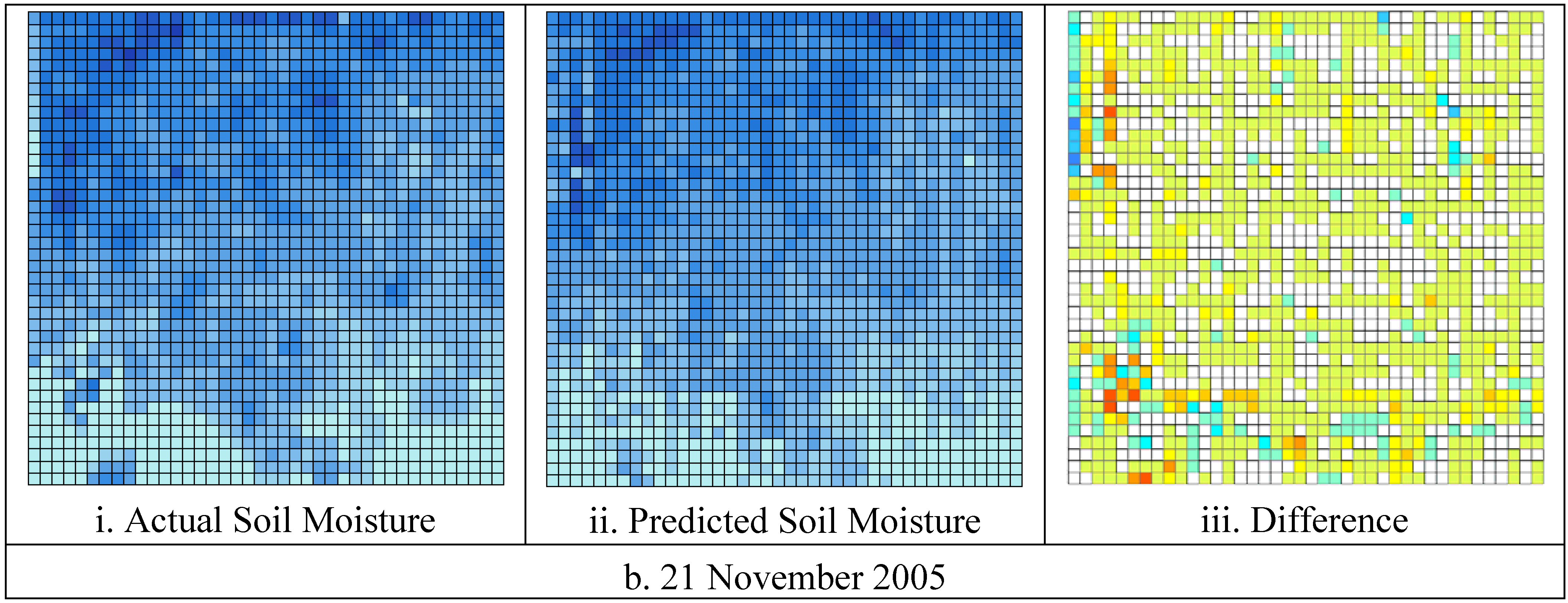
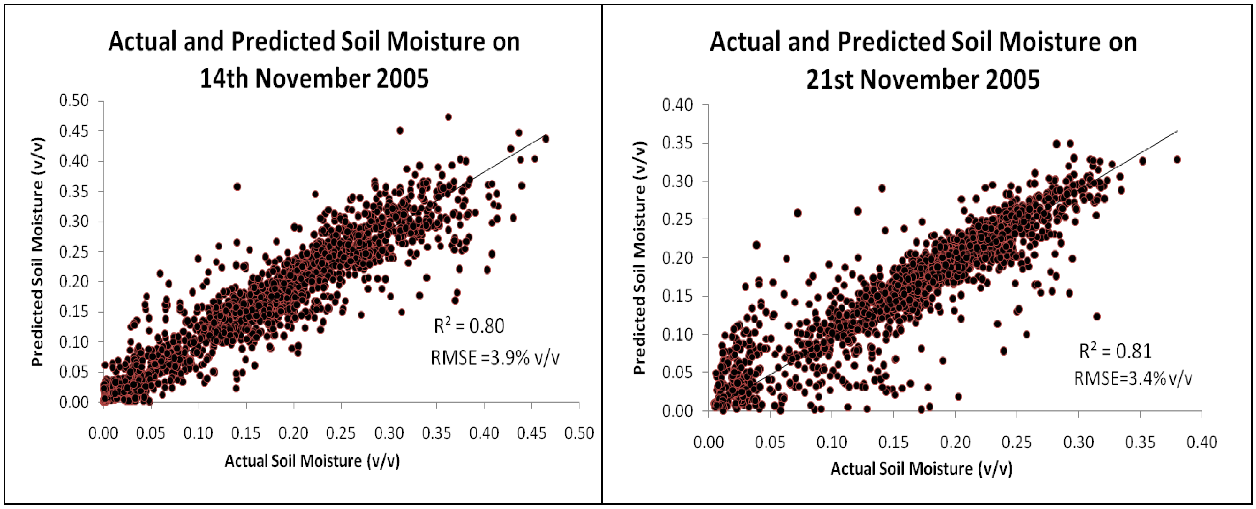
Using this methodology, the RMSE between the actual and predicted values were 3.9% v/v with R² = 0.80 for the 14 November 2005 and 3.4% v/v with R² = 0.88 for the 21 November 2005 respectively. The actual and predicted soil moisture maps are shown in Figure 5, while the correlation relationships are shown using scatter plots in Figure 6. The correlation coefficients chart shows that the predicted and actual soil moisture values are linearly correlated.

Figure 5. Actual and predicted soil moisture map at 1 km resolution on a. 14 November 2005, and b. 21 November 2005.

Figure 5. Actual and predicted soil moisture map at 1 km resolution on a. 14 November 2005, and b. 21 November 2005.

Figure 6. Relationships between referenced and predicted soil moisture value on 14 and 21 November 2005.

Figure 6. Relationships between referenced and predicted soil moisture value on 14 and 21 November 2005.

4.3. Verification: Standardization Factors and Sub-Grid

To verify the use of different standardization factors and sub-grid sizes, a series of experiments were conducted. The ANN of two inputs, one hidden layer of 20 neurons and one output, was trained using data from the 7 November 2005. In contrast to Section 4.2., the standardization factors for the inputs and output of the training data set is reserved to be used for the evaluation cases. This is shown in Figure 7. The trained ANN was then evaluated using the data from the 14 and 21 November 2005, with the evaluation divided into two categories: (i) without sub-grid, and (ii) with sub-grid. The difference between these two categories was that the soil moisture was either retrieved at each of the 1 km cells for the whole target area of 40 km × 40 km (category (i)), or at each of the 1 km cell within the 4 km × 4 km sub-grid. For category (i), the mean and standard deviation values were calculated for the whole 40 km × 40 km area while for category (ii), these statistics values were calculated from each of the 4 km × 4 km sub-grids.

From Table 8, it is clear that with the same standardization factors across the dates, the retrieval accuracies were around 6–9% v/v, which was beyond the acceptable error. Moreover, Table 8 also shows that the use of sub-grid areas does not help to improve the retrieval accuracy when the standardization factors are the same across the dates. The use of the sub-grids is mainly to do with dealing with spatial variation. When the same standardization factors were used, the temporal variation across the dates was not captured. With same standardization factors, i.e., standardization factors obtained from the training data, the retrieval results were the same for both with and without the use of sub-grid. This is as predicted as the de-standardization process was done using the same “scaling factor” from the training data for both with and without sub-grid categories.

Figure 7. The standardization factors from the training data that were used for the verification cases.

Figure 7. The standardization factors from the training data that were used for the verification cases.

Table 8. Results of using same and different standardization factors from the training data for cases of with and without region divisions.

		Same standardization factors		Different standardization factors
		Without sub-grids	With Sub-grids	Without sub-grids	With Sub-grids
14 November	RMSE (%v/v)	6.1	6.1	5.5	3.9
	R2	0.78	0.78	0.72	0.80
21 November	RMSE (%v/v)	8.8	8.8	4.6	3.4
	R2	0.53	0.53	0.65	0.81

Table 8. Results of using same and different standardization factors from the training data for cases of with and without region divisions.

		Same standardization factors		Different standardization factors
		Without sub-grids	With Sub-grids	Without sub-grids	With Sub-grids
14 November	RMSE (%v/v)	6.1	6.1	5.5	3.9
	R2	0.78	0.78	0.72	0.80
21 November	RMSE (%v/v)	8.8	8.8	4.6	3.4
	R2	0.53	0.53	0.65	0.81

A further analysis was carried out using different standardization factors for each evaluation date, but with the retrieval of the 1 km resolution soil moisture undertaken for the whole 40 km × 40 km at once, i.e., without sub-grid division. For this experiment, the temporal variation was captured using the different standardization factors but the spatial variation was neglected (i.e., without the use of sub-grid division). The results of this experiment are in Table 8, showing that the retrieval accuracies were improved (4.6% v/v and 5.5% v/v), but still beyond the acceptable retrieval error. The retrieval results were the best with the use of the proposed methodology of combining the sub-grid and different standardization factor methods.

4.4. Sensitivity: Accuracy of Mean and Standard Deviation Values

A priori information required by this methodology is information about the mean and standard deviation of the soil moisture at each of the sub-grid sizes. While this paper assumed such information was equal to the values calculated from the soil moisture within the sub-grid, such data will not be available in practice, and the mean and standard deviation of sub-grid moisture will need to be estimated from alternative means. Consequently, the sensitivity of results to the accuracy of these values was assessed. Multiple regression method was applied to regress the soil moisture values from TbH, TbV, NDVI and LST values. For each of the dates, 18 data (around 1%) of the data were randomly selected for the regression purpose. The rationale behind the small number of data selected is to simulate a situation where these data were ground-truth data. With more data selected, the regression formula will be more accurate, but at the same time, more sample points will need to be taken if ground sampling is taking place. The RMSE and R² between the actual and regressed soil moisture values are shown in Table 9.

Table 9. RMSE and R² between the regressed and actual soil moisture values.

Date	Linear Regression		With ANN
			Regressed and Predicted		Actual and Predicted
	RMSE (% v/v)	R2	RMSE (% v/v)	R2	RMSE (% v/v)	R2
14 November 2005	8.3	0.77	4.2	0.66	7.8	0.67
21 November 2005	6.0	0.70	1.4	0.92	5.8	0.53

Table 9. RMSE and R² between the regressed and actual soil moisture values.

Date	Linear Regression		With ANN
			Regressed and Predicted		Actual and Predicted
	RMSE (% v/v)	R2	RMSE (% v/v)	R2	RMSE (% v/v)	R2
14 November 2005	8.3	0.77	4.2	0.66	7.8	0.67
21 November 2005	6.0	0.70	1.4	0.92	5.8	0.53

The trained ANN from Section 4.2 is evaluated using the regressed soil moisture values. The results are given in Table 9, showing that the accuracy of the predicted soil moisture with this methodology depends greatly on the mean and standard deviations. The predicted soil moisture values using ANN produce errors that are comparable to the error between the regressed and actual soil moisture values. From this experiment, it is clear that the application of this method depends on the accuracy of the mean and standard deviation values of soil moisture used. Large errors in these spatial statistics will result in large errors in the soil moisture retrieval accuracy when applying this proposed methodology.

5. Conclusions

This paper has presented a methodology which combines variability as the standardization factors together with sub-regional division method, yielding soil moisture retrieval with an acceptable error when testing with field data. The effects of different standardization factors both with and without sub-regional divisions were also shown and discussed. Compared to the usual ANN application to soil moisture retrieval, the combination of these two methods has solved the problem of “out-of-range” conditions when the trained ANN is used for data that is totally new and not previously “seen” by the ANN during the training process. The typical “out-of-range” conditions are mainly due to the inability of the ANN to capture the spatial and temporal variability of the soil moisture. Temporal variability is a common condition in soil moisture retrieval problems when retrieval is needed for dates different from that used in the training process, as it is not easy to cover all the possible conditions during the training. The surface soil moisture variance observed within a square meter (i.e., the spatial variability) can be as large as for a whole field, whereas in this research study, the target area is 40 km × 40 km in size. The methodology proposed in this paper has solved both of these problems. Despite the encouraging results, the main challenge of this method is the accurate estimation of the spatial variability in terms of the mean and standard deviation of the soil moisture as the standardization factors for the ANN. Although the mean and standard deviation within a pre-determined sub-grid size was calculated using the actual soil moisture values in this paper, a sensitivity analysis showed that the methodology depends highly on the accuracy of these two values. Consequently, the proposed approach is highly dependent on the accurate knowledge of the mean and standard deviation of the soil moisture values. Therefore, this method may be more appropriate for soil moisture downscaling.