Seven Years’ Observation of Mid-Upper Tropospheric Methane from Atmospheric Infrared Sounder

 ,
,
Abstract
:1. Introduction
2. Characteristics of CH4 Retrieval from AIRS
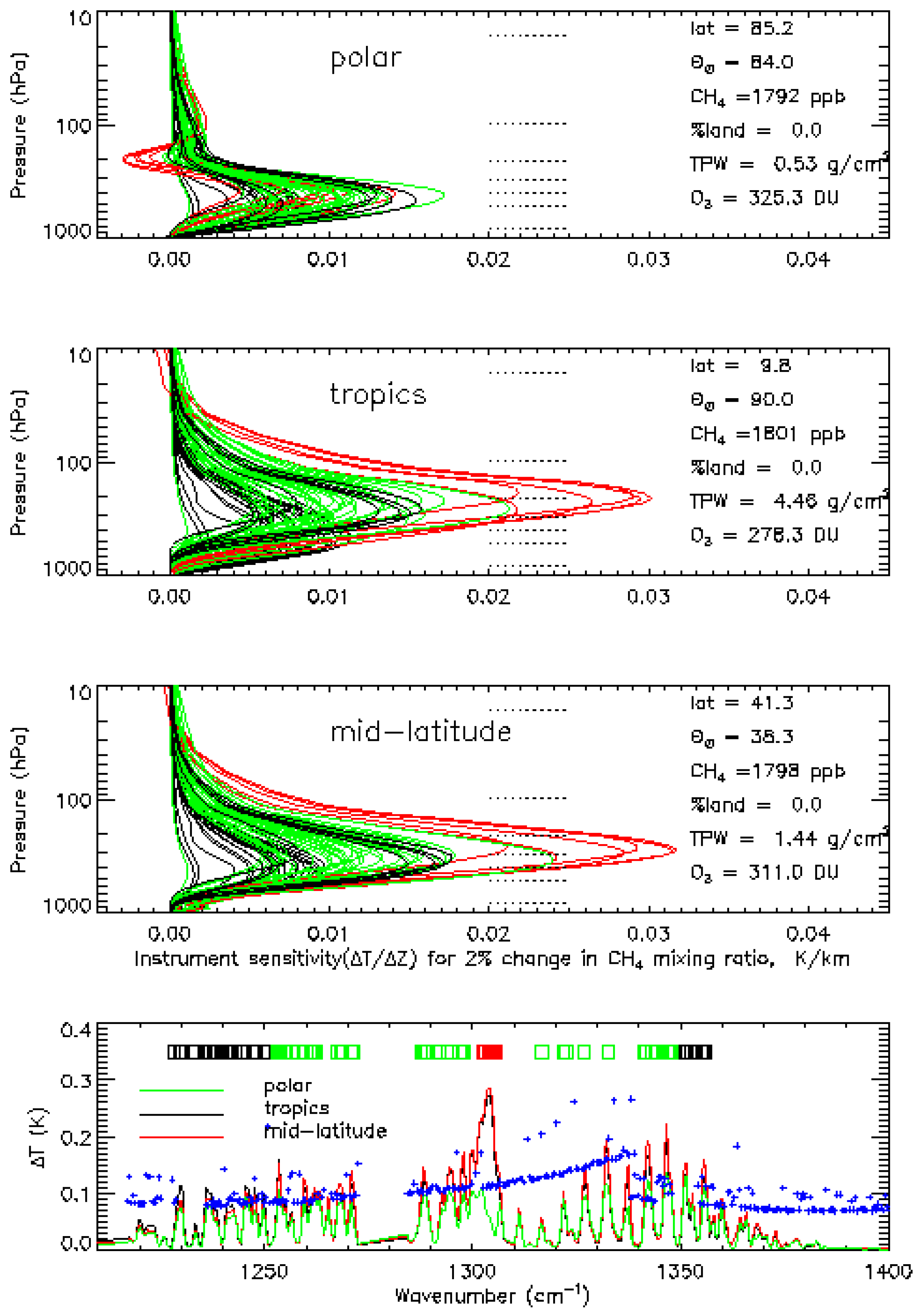
2.1. Sensitivities of AIRS
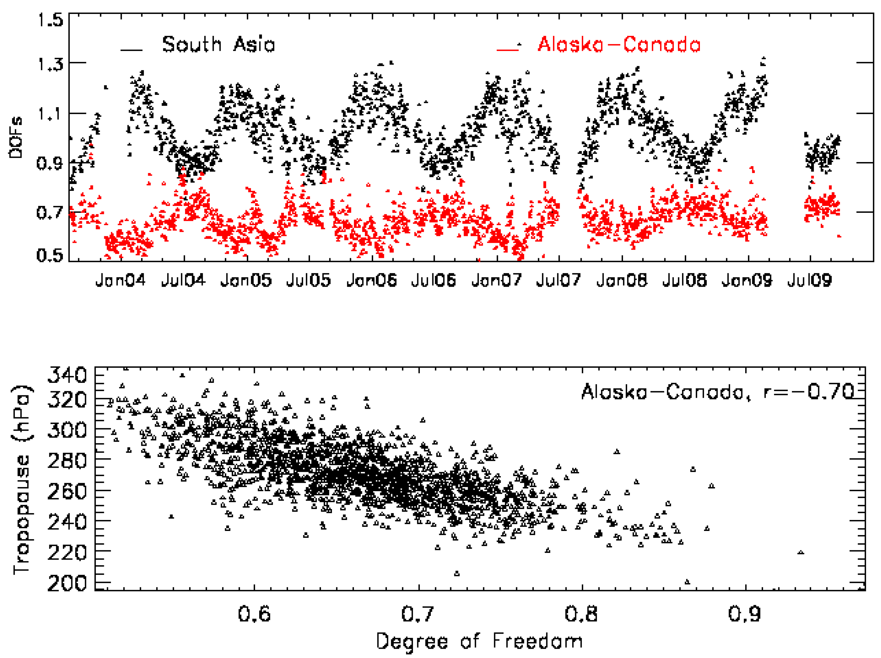
2.2. Variation of Degree of Freedom (DOF)
3. Validation of AIRS CH4
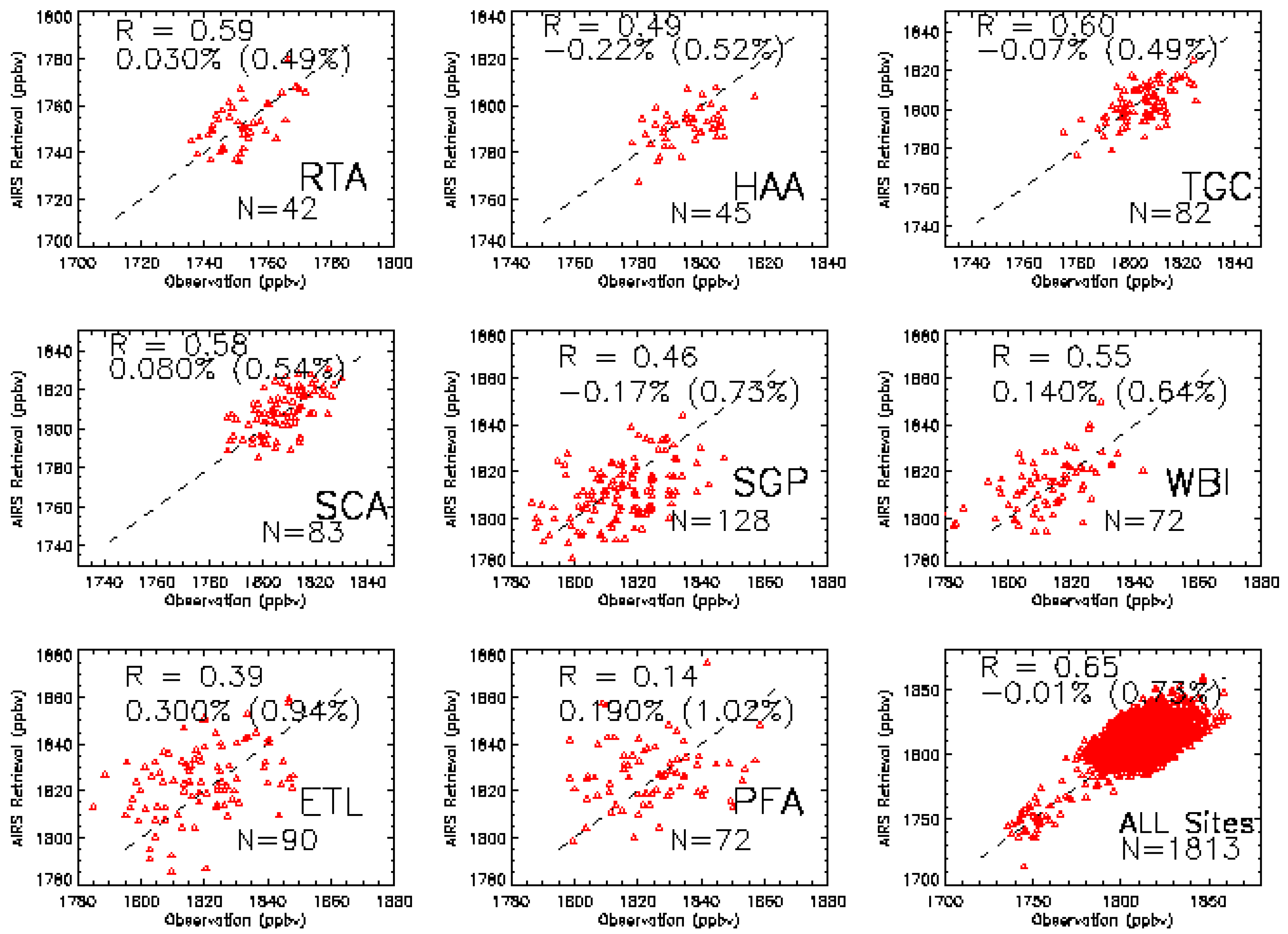
3.1. Validation Data Set
- (1)
- NOAA/ESRL/GMD aircraft measurements: Air samples are collected using turboprop aircraft with maximum altitude limits of 300–350 hPa. Individual flights required about 1.5 hours to complete. Measurements are made by collecting samples of air (approximately 0.7 liter volume at 40 psa) in glass containers. Twelve to twenty flasks are held in a suitcase-sized container, and collection of air in a single flask at a unique altitude allows a sampling vertical resolution of up to 400 m in the boundary layer. After each flight the flask packages are shipped to the NOAA laboratory in Boulder, Colorado for trace gas analysis. Table 1 lists the locations of these sites and their profile number used in validation.
- (2)
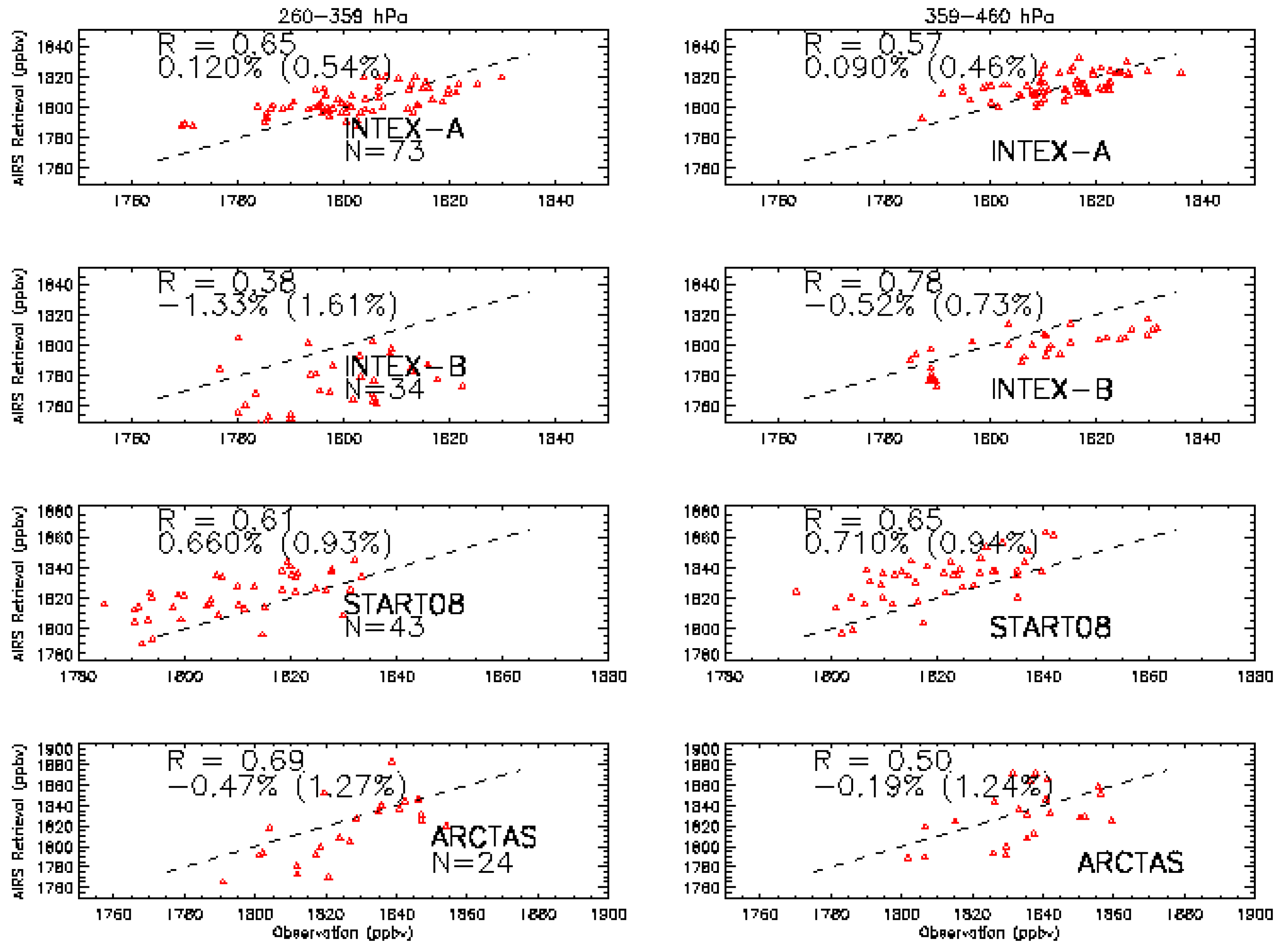
- The INTEX-A field mission was conducted in the summer of 2004 (1 July to 15 August 2004) over North America (NA) and the Atlantic. This effort had a broad scope to investigate the transport and chemistry of long-lived greenhouse gases, oxidants and their precursors, aerosols and their precursors, as well their relationship with radiation and climate. NASA’s DC-8 and J-31 were joined by aircraft from a large number of European and North American partners to explore the composition of the troposphere over NA and the Atlantic as well as radiative properties and effects of clouds and aerosols in a coordinated manner [24]. An air sample is collected in a conditioned, evacuated 2-L stainless steel canister equipped with a bellows valve, and is returned to the UC-Irvine laboratory for CH4 analysis using gas chromatography (GC, HP-5890A) with flame ionization detection. The use of the primary CH4 calibration standards dating back to late 1977 ensures that these measurements are internally consistent. The measurement accuracy is ±1% and the analytical precision at atmospheric mixing ratios is about 1 ppbv [6,25].
- (3)
- INTEX-B was a major NASA led multi-partner atmospheric field campaign completed in the spring of 2006 (http://cloud1.arc.nasa.gov/intex-b/). INTEX-B was performed in two phases. In its first phase (1–21 March), INTEX-B operated as part of the MILAGRO campaign with a focus on observations over Mexico and the Gulf of Mexico. In the second phase (17 April–15 May), the main INTEX-B focus was on trans-Pacific Asian pollution transport. Multiple airborne platforms carrying state of the art chemistry and radiation payloads were flown in concert with satellites and ground stations during the two phases of INTEX-B [26]. The CH4 aircraft measurements in INTEX-B are similar to INTEX-A.
- (4)
- START08 was conducted using the NSF/NCAR Gulfstream V research aircraft during April–June 2008 [27]. START08 was designed to study the chemical transport characteristics of the extratropical upper troposphere and lower stratosphere region. A total of 18 research flights covered a large region of North America (25–65°N in latitude and up to 14.3 km vertical range). Methane was measured in situ by the Unmanned Aircraft Systems Chromatograph for Atmospheric Trace Species. The 2-channel gas chromatograph employed a N2O-doped electron capture detector to measure methane at intervals of 140 s. The measurements were calibrated in-flight using whole air standards.
- (5)
- The ARCTAS mission was conducted in April and June–July 2008 by the Global Tropospheric Chemistry Program and the Radiation Sciences Program of NASA. Its objective was to better understand the factors driving current changes in Arctic atmospheric composition and climate. Three research aircrafts (DC-8, P-3, B-200) were used and a total of 24 research flights had been made. The aircraft were based in Alaska in April (ARCTAS-A) and in western Canada in June–July (ARCTAS-B). The DACOM instrument used is an infrared tunable diode laser absorption spectrometer which makes measurements of CH4 (as well as CO and N2O) at a 1 Hz sample rate. The CH4 accuracy is tied to NOAA/ESRL/GMD carbon cycle group standards and is nominally 1%, and the precision is 0.1% (1 sec, 1 sigma). CH4 observations during ARCTAS-A showed little variability and no indication of significant April emissions from Arctic ecosystems. The July observations in ARCTAS-B over the Hudson Bay Lowlands revealed higher wetland emissions of methane than previously recognized [28].

| CODE | Location | Latitude, Longitude | Profiles used |
|---|---|---|---|
| AAO | Bondville, IL, United States | 40.05, −88.37 | 202 |
| BGI | Bradgate, IA, United States | 42.82, −94.41 | 23 |
| BNE | Beaver Crossing, NE, United States | 40.80, −97.18 | 73 |
| BRM | BERMS, SK, Canada | 54.34, −104.99 | 9 |
| CAR | Briggsdale, CO, United States | 40.37, −104.30 | 124 |
| CMA | Cape May, NJ, United States | 38.83, −74.32 | 87 |
| DND | Dahlen, ND, United States | 48.14 , −97.99 | 76 |
| ESP | Estevan Point, BC, Canada | 49.58, −126.37 | 131 |
| ETL | East Trout Lake, SK, Canada | 54.35, −104.98 | 90 |
| FWI | Fairchild, WI, United States | 44.66, −90.96 | 24 |
| HAA | Molokai Island, HI, United States | 21.23, −158.95 | 45 |
| HFM | Harvard Forest, MA, United States | 42.54, −72.17 | 49 |
| HIL | Homer, IL, United States | 40.07, −87.91 | 85 |
| LEF | Park Falls, WI, United States | 45.93, −90.27 | 122 |
| NHA | Worcester, MA, United States | 42.95, −70.63 | 67 |
| NWR | Niwot Ridge, CO, United States | 40.05, −105.58 | 45 |
| OIL | Oglesby, IL, United States | 41.28, −88.94 | 35 |
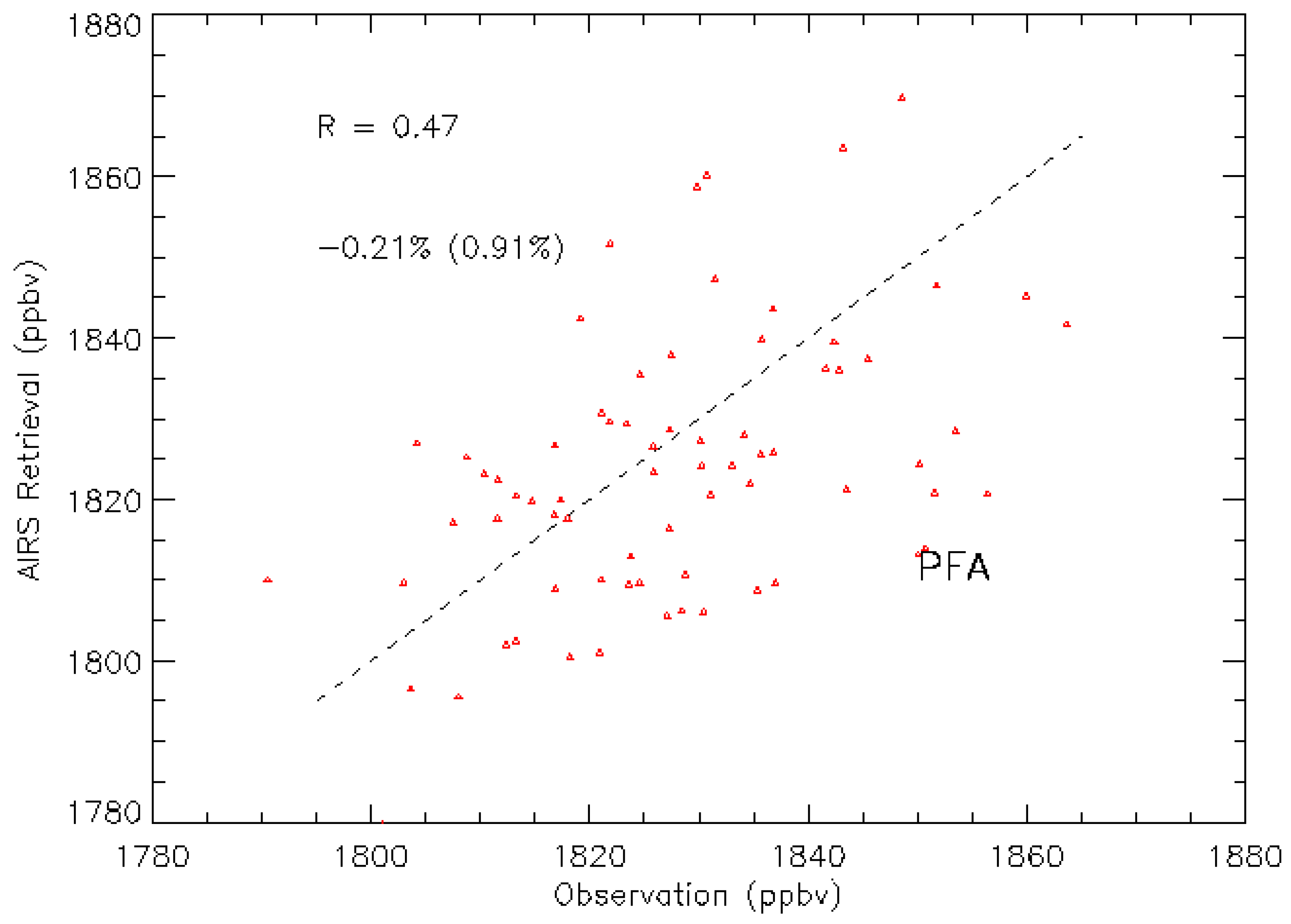
| PFA | Poker Flat, AL, United States | 65.07, −147.29 | 72 |
| RIA | Rowley, IA, United States | 42.40, −91.84 | 26 |
| RTA | Rarotonga, Cook Islands | −21.25, −159.83 | 42 |
| SCA | Charleston, SC, United States | 32.77, −79.55 | 83 |
| SGP | Southern Great Plains, OK, United States | 36.80, −97.50 | 128 |
| TGC | Sinton, TX, United States | 27.73, −96.86 | 82 |
| THD | Trinidad Head, CA, United States | 41.054, −124.151 | 70 |
| VAA | Cartersville, GA, United States | 32.91, −79.36 | 8 |
| WBI | West Branch, IO, United States | 41.725, −91.353 | 72 |
3.2. Validation Results


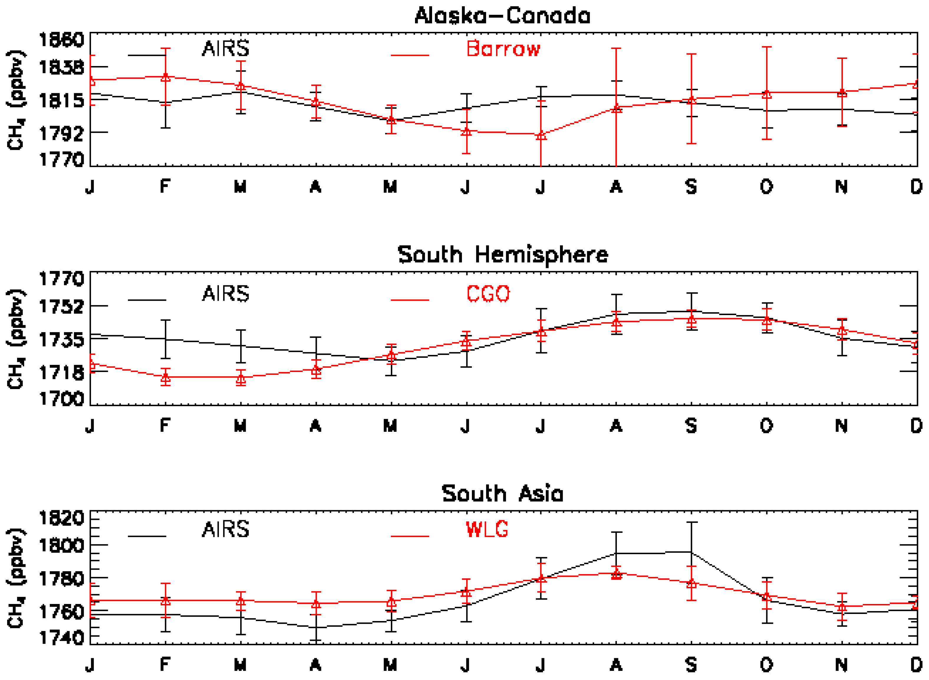
3.3. The Representative Layer in the AIRS Retrieved CH4 Profile for Scientific Analysis in the HNH
4. Multi-Year MUT-CH4 Mixing Ratios from AIRS Observations, Seasonal Cycle and its Increase in 2008–2009
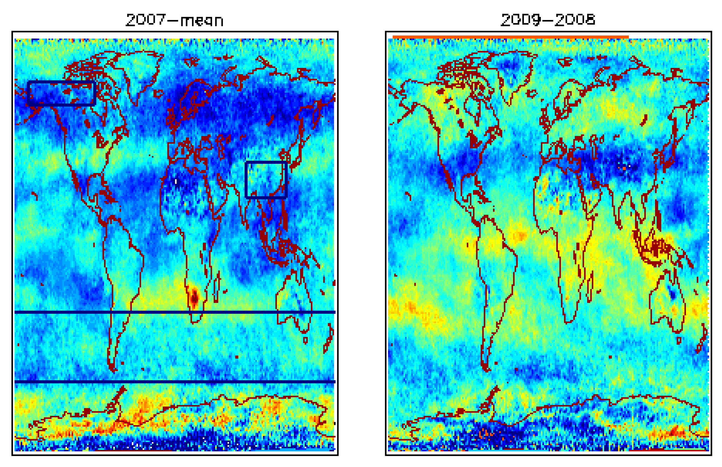
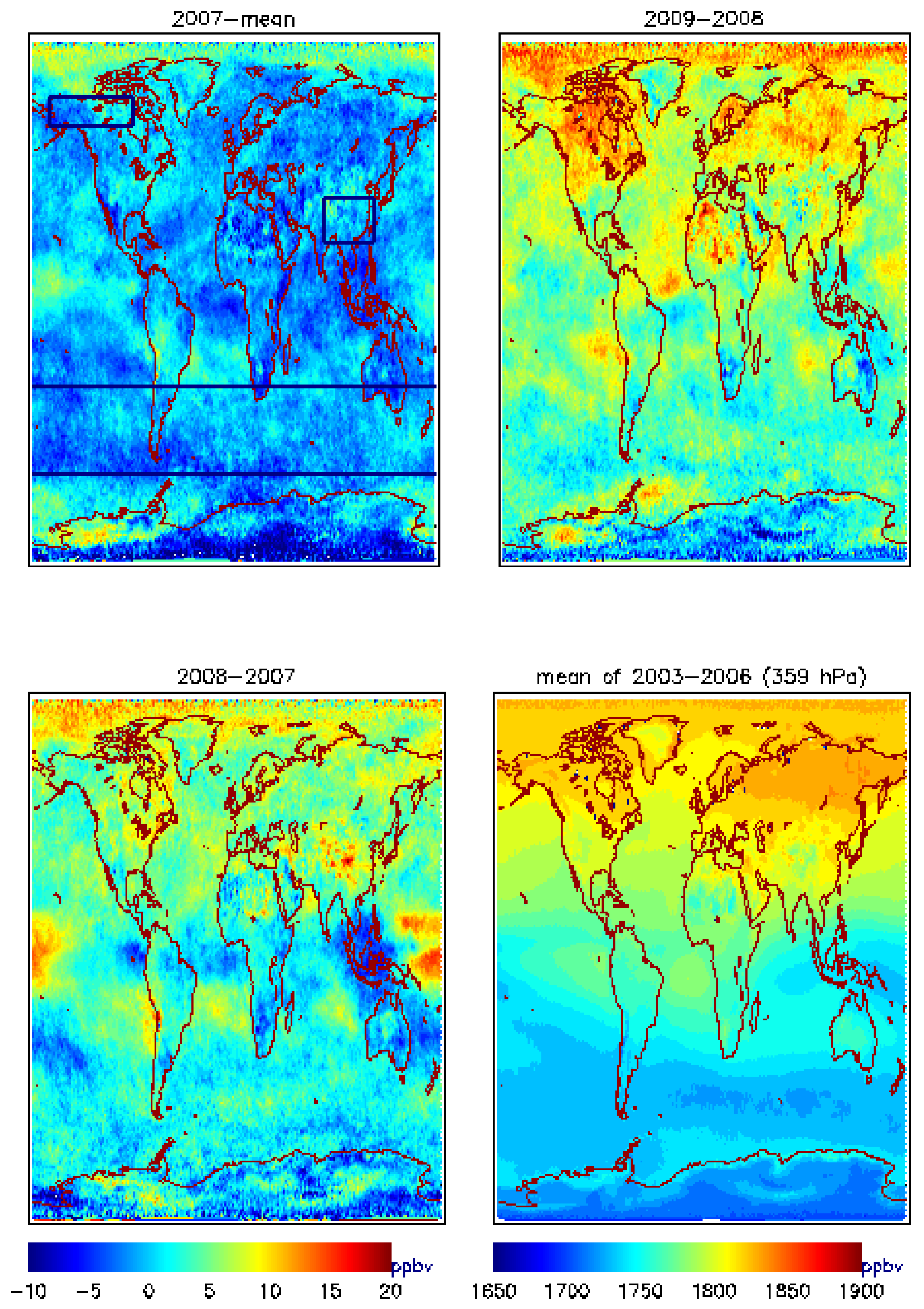
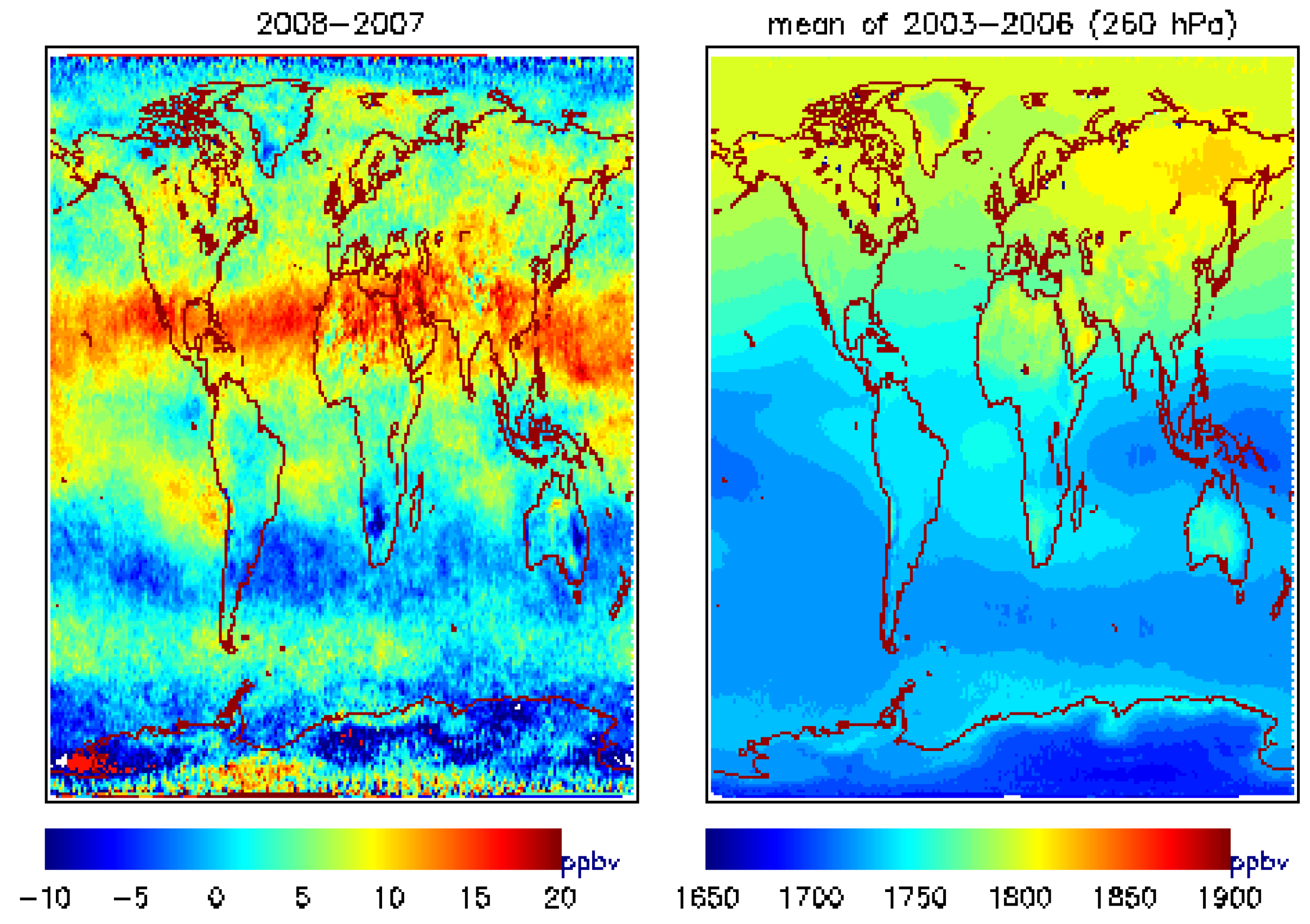
4.1. Global View of MUT-CH4 and Its Increase during 2007–2009
| 2007 | 2008 | 2009 | |
| Alaska-Canada | −0.32(1.06) | 5.42(4.93) | 5.89(5.11) |
| South Asia | −1.58 (0.93) | 12.89(7.0) | −0.29 (0.09) |
| South Hemisphere | −1.63(−0.48) | 1.92(3.06) | 3.53(1.65) |


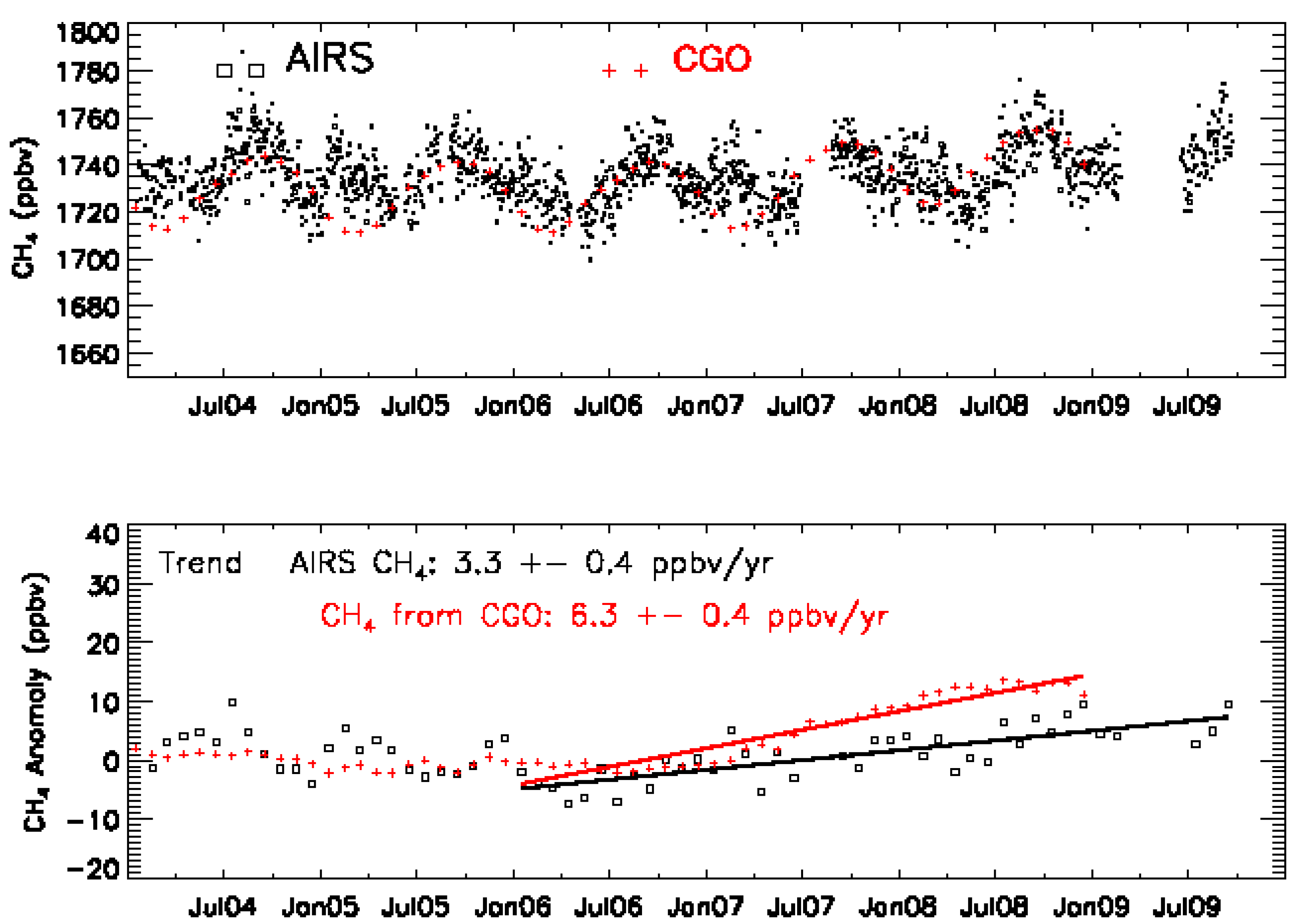
4.2.MUT-CH4 in Southern Hemisphere
4.3. MUT-CH4 in South Asia

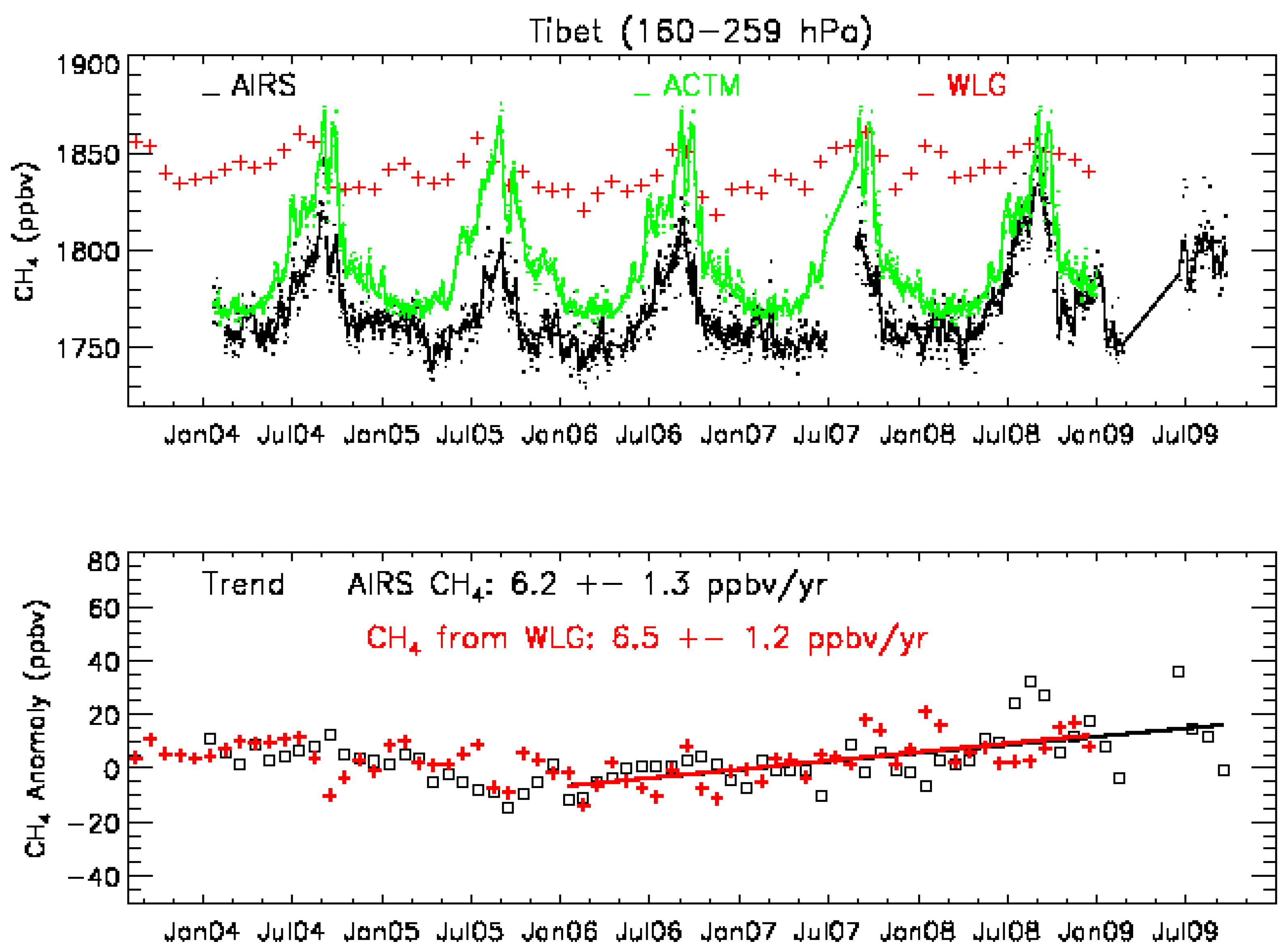
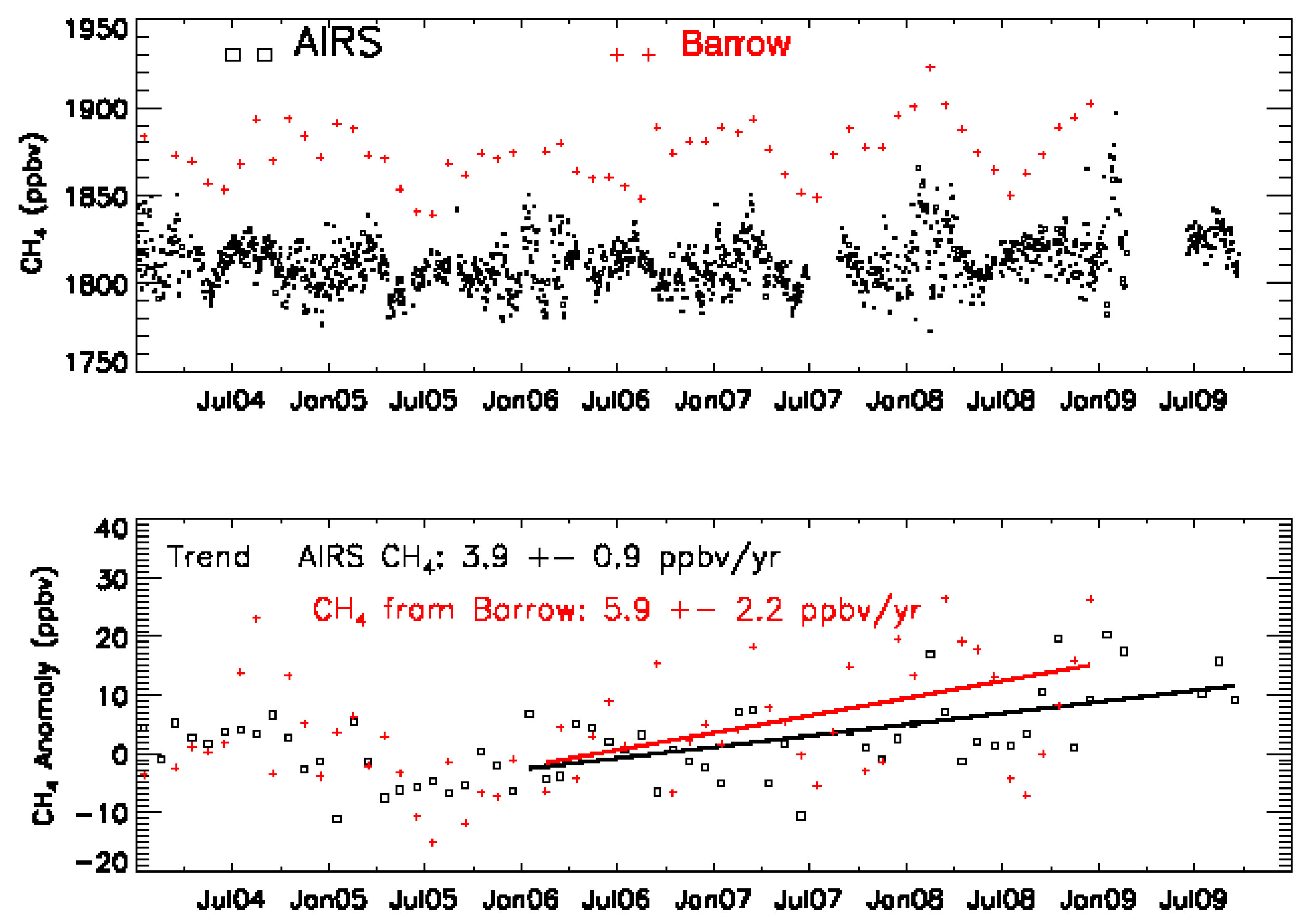
4.4. MUT-CH4 in the HNH

4.5. Seasonal Cycle of MUT-CH4

5. Summary and Conclusions
Acknowledgements
References
- Solomon, S.; Qin, D.; Manning, M.; Chen, Z.; Marquis, M.; Averyt, K.B.; Tignor, M.; Miller, H.L. Climate Change 2007: The Physical Science Basis: Contribution of Working Group I to the Fourth Assessment Report of the Intergovernmental Panel on Climate Change; Cambridge University Press: Cambridge, UK and New York, NY, USA, 2007; p. 996. [Google Scholar]
- Rasmussen, R.A.; Khalil, M.A.K. Atmospheric methane in recent and ancient atmospheres: Concentrations, trends, and interhemispheric gradient. J. Geophys. Res. 1984, 89, 11599–11605. [Google Scholar] [CrossRef]
- Nakazawa, T.; Machida, T.; Tanaka, M.; Fujii, Y.; Aoki, S.; Watanabe, O. Differences of the atmospheric CH4 concentration between the Arctic and Antarctic regions in pre-industrial/pre-agricultural era. Geophys. Res. Lett. 1993, 20, 943–946. [Google Scholar] [CrossRef]
- Dlugokencky, E.J.; Steele, L.P.; Lang, P.M.; Masarie, K.A. The growth rate and distribution of atmospheric methane. J. Geophys. Res. 1994, 99, 17021–17044. [Google Scholar] [CrossRef]
- Dlugokencky, E.J.; Houweling, S.; Bruhwiler, L.; Masarie, K.A.; Lang, P.M.; Miller, J.B.; Tans, P.P. Atmospheric methane levels off: Temporary pause or a new steady-state? Geophys. Res. Lett. 2003, 30. [Google Scholar] [CrossRef]
- Simpson, I.J.; Chen, T.-Y.; Blake, D.R.; Rowland, F.S. Implications of the recent fluctuations in the growth rate of tropospheric methane. Geophys. Res. Lett. 2002, 29. [Google Scholar] [CrossRef]
- Rigby, M.; Prinn, R.G.; Fraser, P.J.; Simmonds, P.G.; Langenfelds, R.L.; Huang, J.; Cunnold, D.M.; Steele, L.P.; Krummel, P.B.; Weiss, R.F.; O’Doherty, S.; Salameh, P.K.; Wang, H.J.; Harth, C.M.; Mühle, J.; Porter, L.W. Renewed growth of atmospheric methane. Geophys. Res. Lett. 2008, 35. [Google Scholar] [CrossRef]
- Dlugokencky, E.J.; Bruhwiler, L.; White, J.W.C.; Emmons, L.K.; Novelli, P.C.; Montzka, S.A.; Masarie, K.A.; Lang, P.M.; Crotwell, A.M.; Miller, J.B.; Gatti, L.V. Observational constraints on recent increases in the atmospheric CH4 burden. Geophys. Res. Lett. 2009, 36. [Google Scholar] [CrossRef]
- Zhuang, Q.; Melack, J.M.; Zimov, S.; Walter, K.M.; Butenhoff, C.L.; Khalil, M.A.K. Global methane emissions from wetlands, rice paddies, and lakes. Eos Trans. AGU 2009, 90. [Google Scholar] [CrossRef]
- Walter, K.M.; Zimov, S.A.; Chanton, J.P.; Verbyla, D.; Chapin, F.S. Methane bubbling from Siberian thaw lakes as a positive feedback to climate warming. Nature 2006, 443, 71–75. [Google Scholar] [CrossRef]
- Shakhova, N.; Semiletov, I.; Salyuk, A.; Yusupov, V.; Kosmach, D.; Gustafsson, Ö. Extensive methane venting to the atmosphere from sediments of the East Siberian arctic shelf. Science 2010, 327, 1246–1250. [Google Scholar] [CrossRef]
- Frankenberg, C.; Bergamaschi, P.; Butz, A.; Houweling, S.; Meirink, J.F.; Notholt, J.; Petersen, A.K.; Schrijver, H.; Warneke, T.; Aben, I. Tropical methane emissions: A revised view from SCIAMACHY onboard ENVISAT. Geophys. Res. Lett. 2008, 35. [Google Scholar] [CrossRef]
- Yokota, T.; Aoki, T.; Eguchi, N.; Ota, Y.; Yoshida, Y.; Oshchepkov, S.; Bril, A.; Desbiens, R.; Morino, I. Data retrieval algorithms of the SWIR bands of the TANSO-FTS sensor aboard GOSAT. J. Remote Sens. Soc. Jpn 2008, 28, 133–142. [Google Scholar]
- Payne, V.H.; Clough, S.A.; Shephard, M.W.; Nassar, R.; Logan, J.A. Information-centered representation of retrievals with limited degrees of freedom for signal: Application to methane from the Tropospheric Emission Spectrometer. J. Geophys. Res. 2009, 114. [Google Scholar] [CrossRef]
- Aumann, H.H.; Chahine, M.T.; Gautier, C.; Goldberg, M.D.; Kalnay, E.; McMillin, L.M.; Revercomb, H.; Rosenkranz, P.W.; Smith, W.L.; Staelin, D.H.; Strow, L.L.; Susskind, J. AIRS/AMSU/HSB on the aqua mission: Design, science objectives, data products, and processing systems. IEEE Trans. Geosci. Remote Sens. 2003, 41, 253–264. [Google Scholar] [CrossRef]
- Crevoisier, C.; Nobileau, D.; Fiore, A.M.; Armante, R.; Chédin, A.; Scott, N.A. Tropospheric methane in the tropics—First year from IASI hyperspectral infrared observations. Atmos. Chem. Phys. 2009, 9, 6337–6350. [Google Scholar] [CrossRef]
- Razavi, A.; Clerbaux, C.; Wespes, C.; Clarisse, L.; Hurtmans, D.; Payan, S.; Camy-Peyret, C.; Coheur, P.F. Characterization of methane retrievals from the IASI space-borne sounder. Atmos. Chem. Phys. 2009, 9, 7889–7899. [Google Scholar] [CrossRef] [Green Version]
- Aumann, H.H.; Pagano, T.S. Using AIRS and IASI data to evaluate absolute radiometric accuracy and stability for climate applications. Proc. SPIE 2008, 7085. [Google Scholar] [CrossRef]
- Xiong, X.; Barnet, C.; Maddy, E.; Sweeney, C.; Liu, X.; Zhou, L.; Goldberg, M. Characterization and validation of methane products from the Atmospheric Infrared Sounder (AIRS). J. Geophys. Res. 2008, 113. [Google Scholar] [CrossRef]
- Strow, L.L.; Hannon, S.E.; De Souza-Machado, S.; Motteler, H.E.; Tobin, D. An overview of the AIRS radiative transfer model. IEEE Trans. Geosci. Remote Sens. 2003, 41, 303–313. [Google Scholar] [CrossRef]
- Xiong, X.; Barnet, C.; Wei, J.; Maddy, E. Information-based mid-upper tropospheric methane derived from Atmospheric Infrared Sounder (AIRS) and its validation. Atmos. Chem. Phys. Discuss. 2009, 9, 16331–16360. [Google Scholar] [CrossRef]
- Xiong, X.; Barnet, C.; Zhuang, Q.; Machida, T.; Sweeney, C.; Patra, P.K. Mid-upper tropospheric methane in the high northern hemisphere: Space-borne observations by AIRS, aircraft measurements and model simulations. J. Geophys. Res. 2010, 115, D19309. [Google Scholar] [CrossRef]
- Maddy, E.S.; Barnet, C.D. Vertical resolution estimates in Version 5 of AIRS operational retrievals. IEEE Trans. Geosci. Remote Sens. 2008, 46, 2375–2384. [Google Scholar] [CrossRef]
- Singh, H.B.; Brune, W.H.; Crawford, J.H.; Jacob, D.J.; Russell, P.B. Overview of the summer 2004 Intercontinental Chemical Transport Experiment-North America (INTEX-A). J. Geophys. Res. 2006, 111. [Google Scholar] [CrossRef]
- Simpson, I.J.; Rowland, F.S.; Meinardi, S.; Blake, D.R. Influence of biomass burning during recent fluctuations in the slow growth of global tropospheric methane. Geophys. Res. Lett. 2006, 33, L22808. [Google Scholar] [CrossRef]
- Singh, H.B.; Brune, W.H.; Crawford, J.H.; Flocke, F.; Jacob, D.J. Chemistry and transport of pollution over the Gulf of Mexico and the Pacific: Spring 2006 INTEX-B campaign overview and first results. Atmos. Chem. Phys. 2009, 9, 2301–2318. [Google Scholar] [CrossRef]
- Pan, L.L.; Bowman, K.P.; Atlas, E.L.; Wofsy, S.C.; Zhang, F.; Bresch, J.F.; Ridley, B.A.; Pittman, J.V.; Homeyer, C.R.; Romashkin, P.; Cooper, W.A. The Stratosphere-Troposphere analyses of Regional Transport 2008 (START08) Experiment. Bull. Amer. Meteor. Soc. 2010, 91, 327–342. [Google Scholar] [CrossRef]
- Jacob, D.J.; Crawford, J.H.; Maring, H.; Clarke, A.D.; Dibb, J.E.; Ferrare, R.A.; Hostetler, C.A.; Russell, P.B.; Singh, H.B.; Thompson, A.M.; Shaw, G.E.; McCauley, E.; Pederson, J.R.; Fisher, J.A. The ARCTAS aircraft mission: design and execution. Atmos. Chem. Phys. Discuss. 2009, 9, 17073–17123. [Google Scholar] [CrossRef]
- Patra, P.K.; Takigawa, M.; Ishijima, K.; Choi, B.-C.; Cunnold, D.; Dlugokencky, E.J.; Fraser, P.; Gomez-Pelaez, A.J.; Goo, T.-Y.; Kim, J.-S.; Krummel, P.; Langenfelds, R.; Meinhardt, F.; Mukai, H.; O’Doherty, S.; Prinn, R.G.; Simmonds, P.; Steele, P.; Tohjima, Y.; Tsuboi, K.; Uhse, K.; Weiss, R.; Worthy, D.; Nakazawa, T. Growth rate, seasonal, synoptic, diurnal variations and budget of methane in lower atmosphere. J. Meteorol. Soc. Jpn. 2009, 87, 635–663. [Google Scholar] [CrossRef]
- GLOBALVIEW-CH4: Cooperative Atmospheric Data Integration Project—Methane; [CD-ROM], NOAA ESRL: Boulder, CO, USA, 2009.
- Xiong, X.; Houweling, S.; Wei, J.; Maddy, E.; Sun, F.; Barnet, C. Methane plume over south Asia during the monsoon season: Satellite observation and model simulation. Atmos. Chem. Phys. 2009, 9, 783–794. [Google Scholar] [CrossRef]
- Schuck, T.J.; Brenninkmeijer, C.A.M.; Baker, A.K.; Slemr, F.; von Velthoven, P.F.J.; Zahn, A. Greenhouse gas relationships in the Indian summer monsoon plume measured by the CARIBIC passenger aircraft. Atmos. Chem. Phys. 2010, 10, 3965–3984. [Google Scholar] [CrossRef]
© 2010 by the authors; licensee MDPI, Basel, Switzerland. This article is an open access article distributed under the terms and conditions of the Creative Commons Attribution license (http://creativecommons.org/licenses/by/3.0/).
Share and Cite
Xiong, X.; Barnet, C.; Maddy, E.; Wei, J.; Liu, X.; Pagano, T.S. Seven Years’ Observation of Mid-Upper Tropospheric Methane from Atmospheric Infrared Sounder. Remote Sens. 2010, 2, 2509-2530. https://0-doi-org.brum.beds.ac.uk/10.3390/rs2112509
Xiong X, Barnet C, Maddy E, Wei J, Liu X, Pagano TS. Seven Years’ Observation of Mid-Upper Tropospheric Methane from Atmospheric Infrared Sounder. Remote Sensing. 2010; 2(11):2509-2530. https://0-doi-org.brum.beds.ac.uk/10.3390/rs2112509
Chicago/Turabian StyleXiong, Xiaozhen, Chris Barnet, Eric Maddy, Jennifer Wei, Xingpin Liu, and Thomas S. Pagano. 2010. "Seven Years’ Observation of Mid-Upper Tropospheric Methane from Atmospheric Infrared Sounder" Remote Sensing 2, no. 11: 2509-2530. https://0-doi-org.brum.beds.ac.uk/10.3390/rs2112509