Evidence of Hydroperiod Shortening in a Preserved System of Temporary Ponds


Abstract
:
1. Introduction
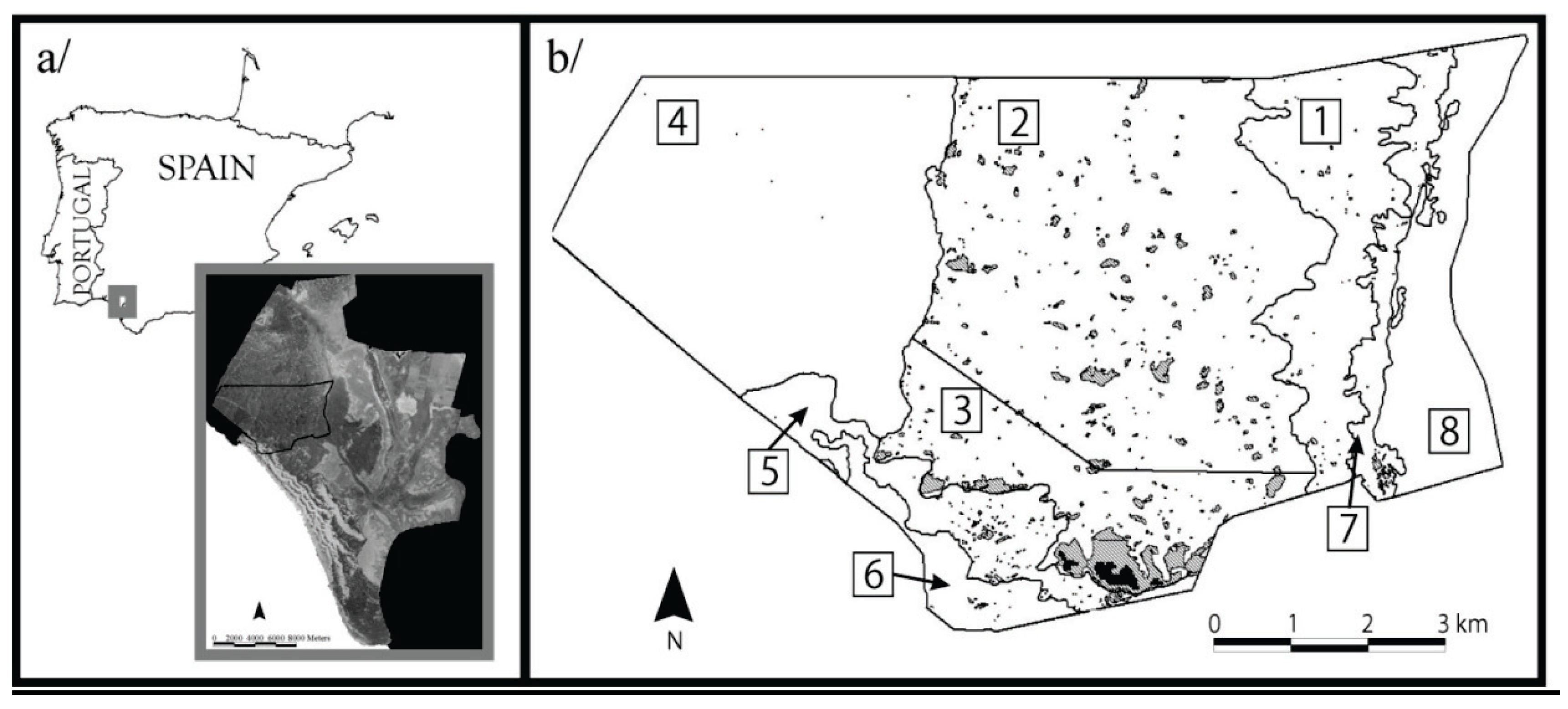
2. Study Area

3. Methods
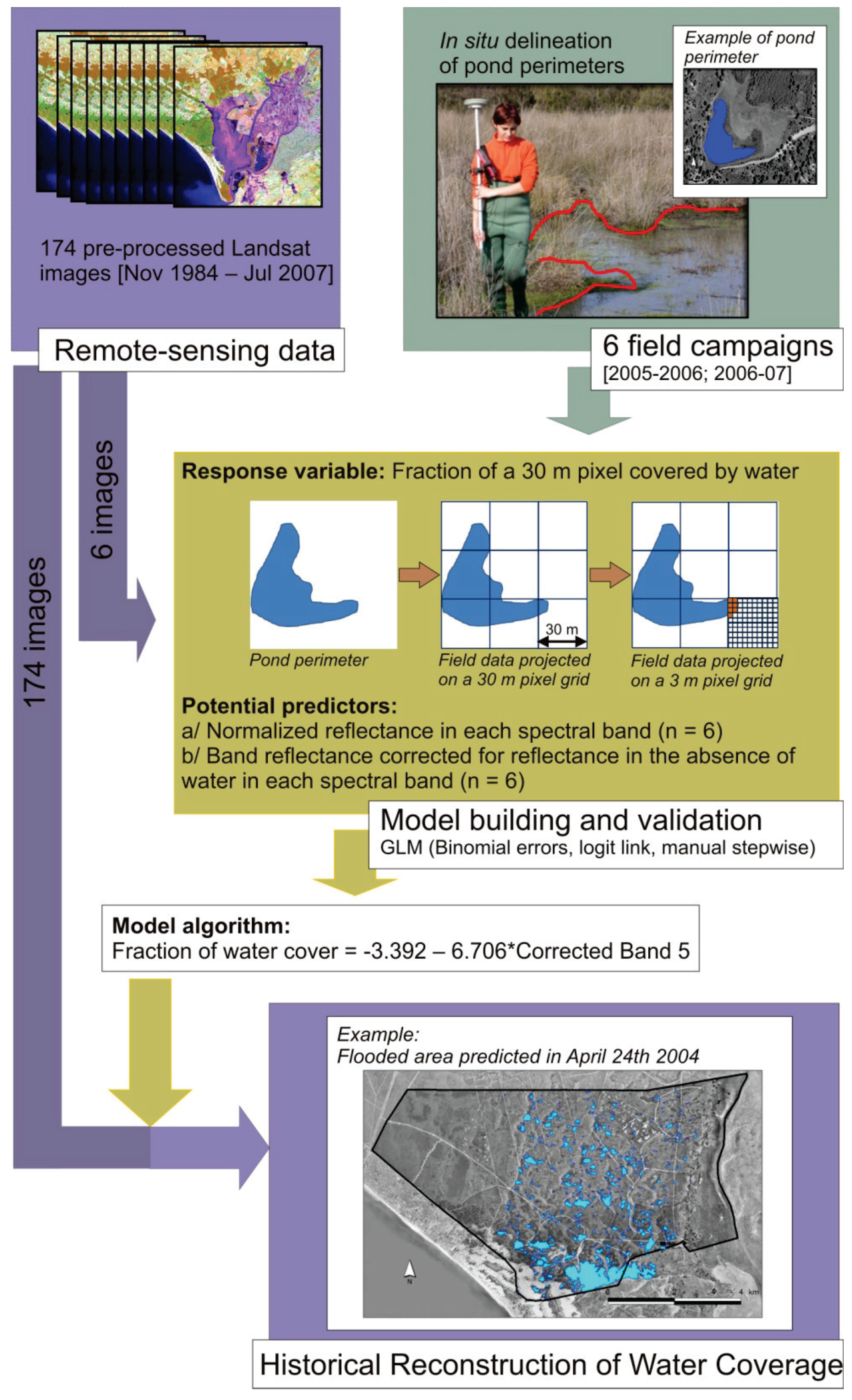
3.1. Pre-Processing of Time-Series Landsat Images
3.2. Ground-Truth Data: In Situ Delineation of Flooded Area
3.3. Model Development and Validation
3.3.1. Model Building
3.3.2. Model Validation


| Adjusted model parameters | ||||
|---|---|---|---|---|
| Final model parametization | F | df | p | |
| Fraction of water cover = −3.392 − 6.706×CB5 | 1,215.70 | 1,1817 | 0.001 | |
| Manual step-wise predictor selection (Explained deviance [%]) | ||||
| Band (B) | Corrected band (CB) | |||
| Band 1 (λ = 0.45 − 0.52 µm) | 8.81 | 15.23 | ||
| Band 2 (λ = 0.52 − 0.60 µm) | 14.86 | 22.22 | ||
| Band 3 (λ = 0.63 − 0.69 µm) | 19.24 | 32.00 | ||
| Band 4 (λ = 0.76 − 0.90 µm) | 41.57 | 43.43 | ||
| Band 5 (λ = 1.55 − 1.75 µm) | 36.49 | 47.09 | ||
| Band 7 (λ = 2.08 − 2.35 µm) | 25.93 | 33.86 | ||
3.4. Historical Reconstruction of Water Coverage in the Study Area (November 1984–July 2007)
3.5. Spatio-Temporal Variation in the Distribution of Water
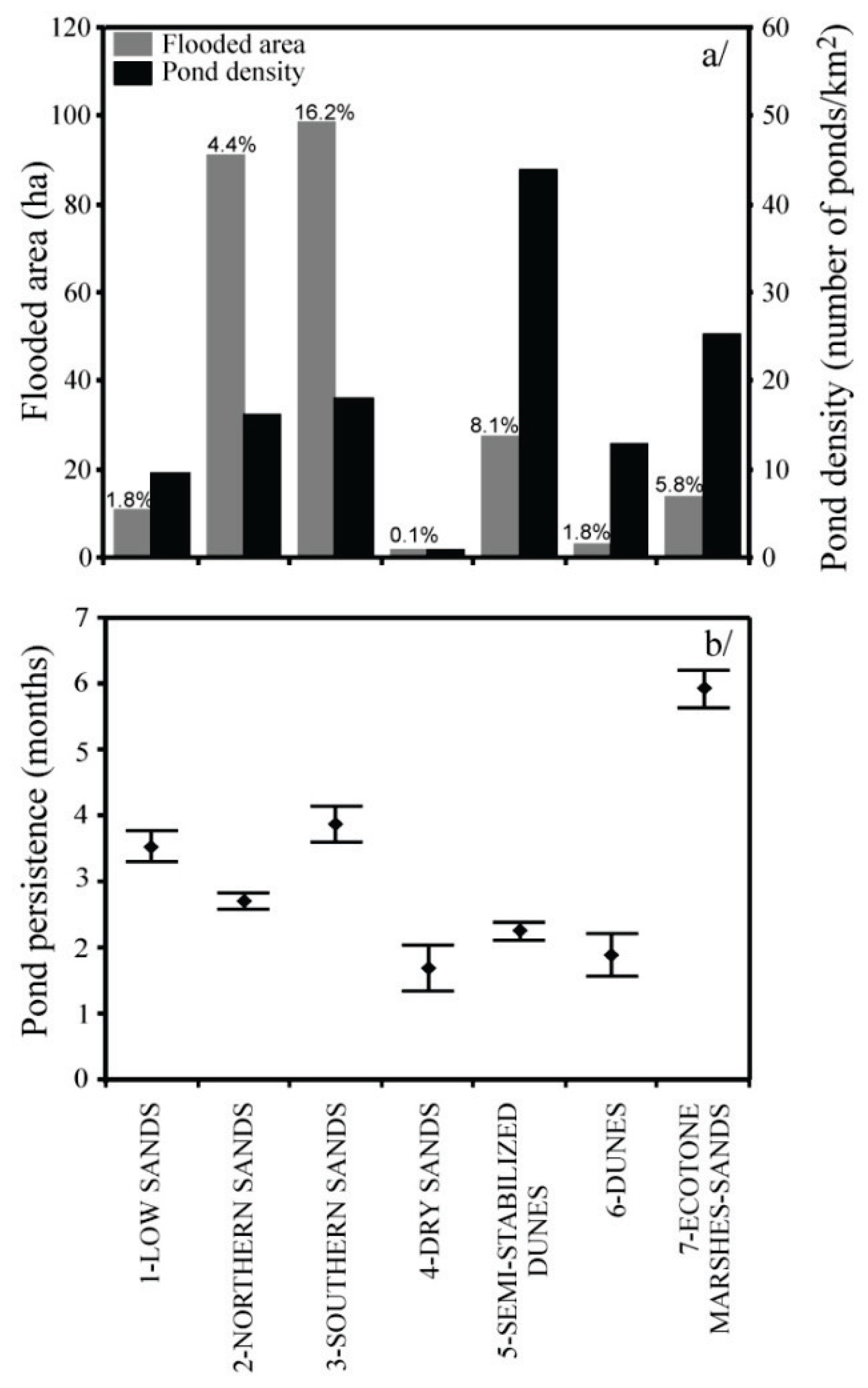
3.5.1. Differences in Hydrologic Behavior among Ecosections
3.5.2. Seasonal Hydrologic Behavior of Temporary Ponds
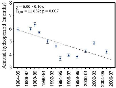
3.5.3. Inter-Annual Variation in Hydrologic Behavior
3.5.4. Relationship between Flooded Area and Rainfall
4. Results
4.1. Model Development and Validation
| MODEL VALIDATION CIRCUMSTANCES | |||||
|---|---|---|---|---|---|
| Predictions | Pixels | N | Spearman R | p | |
| 1 | Raw | All | 5,778 | 0.367 | < 0.001 |
| 2 | Raw | Potentially flooded | 2,897 | 0.457 | < 0.001 |
| 3 | Modified | All | 5,778 | 0.502 | < 0.001 |
| 4 | Modified | Potentially flooded | 2,897 | 0.562 | < 0.001 |
4.2. Historical Reconstruction of Water Coverage in the Study Area
| Observed temporary ponds | ||||
| Dry | Flooded | Total | ||
| Predicted temporary ponds | Dry | 64 | 33 | 97 |
| Flooded | 14 | 57 | 71 | |
| Total | 78 | 90 | 168 | |
| Correct classification | 82% | 63% | 72% | |
4.3. Spatio-Temporal Variation in the Distribution of Water
4.3.1. Differences in Hydrologic Behavior among Ecosections


4.3.2. Seasonal Hydrologic Behavior of Temporary Ponds.

4.3.3. Inter-Annual Variation in Hydrologic Behavior
4.3.4. Relationship between Flooded Area and Rainfall

| Flooded area | Annual hydroperiod | ||||||
|---|---|---|---|---|---|---|---|
| Model parameterization | F (df) | p | Model parameterization | F (df) | p | ||
| 1 | LOW SANDS | y = 5.57 + 0.03t | 0.053 (1,21) | 0.820 | y = 5.87 − 0.12t | 3.483 (1,10) | 0.091 |
| 2 | NORTHERN SANDS | y = 36.23 + 0.07t | 0.006 (1,21) | 0.940 | y = 5.81 − 0.10t | 12.728 (1,10) | 0.005 |
| 3 | SOUTHERN SANDS | y = 60.09 + 0.09t | 0.010 (1,21) | 0.921 | y = 7.42 − 0.16t | 11.273 (1,10) | 0.007 |
| 4 | DRY SANDS | y = 1.34 − 0.04t | 4.254 (1,21) | 0.052 | y= 5.78 − 0.15t | 6.761 (1,10) | 0.026 |
| 5 | SEMI-STABILIZED DUNES | y = 10.56 − 0.11t | 0.157 (1,21) | 0.696 | y = 5.01 − 0.12t | 16.765 (1,10) | 0.002 |
| 6 | DUNES | y = 2.04 − 0.06t | 4.409 (1,21) | 0.048 | y = 6.22 − 0.20t | 16.488 (1,10) | 0.002 |
| 7 | ECOTONE MARSHES-SANDS | y= 8.33 + 0.08t | 0.418 (1,21) | 0.524 | y = 6.10 + 0.02t | 0.268 (1,10) | 0.616 |
| Standardized coefficients | R2 | Adj.R2 | F | df1 | df2 | p | |||||||
|---|---|---|---|---|---|---|---|---|---|---|---|---|---|
| P1-15 | P16-30 | P31-90 | P91-180 | P181-365 | P366-730 | ||||||||
| Entire study area | 0.228 | 0.179 | 0.643 | 0.575 | 0.235 | 0.196 | 0.803 | 0.795 | 113.1 | 167 | 6 | < 0.001 | |
| Ecosection | |||||||||||||
| 1 | LOW SANDS | 0.285 | 0.204 | 0.561 | 0.333 | 0.650 | 0.642 | 78.6 | 169 | 4 | < 0. 001 | ||
| 2 | NORTHERN SANDS | 0.244 | 0.144 | 0.629 | 0.399 | 0.107 | 0.144 | 0.653 | 0.641 | 52.4 | 167 | 6 | < 0.001 |
| 3 | SOUTHERN SANDS | 0.193 | 0.165 | 0.587 | 0.639 | 0.347 | 0.237 | 0.778 | 0.770 | 97.6 | 167 | 6 | < 0.001 |
| 4 | DRY SANDS | 0.222 | 0.049 | 0.044 | 8.9 | 172 | 1 | <0.01 | |||||
| 5 | SEMI-STABILIZED DUNES | 0.183 | 0.179 | 0.626 | 0.498 | 0.183 | 0.141 | 0.693 | 0.682 | 62.8 | 167 | 6 | < 0.001 |
| 6 | DUNES | 0.146 | 0.432 | 0.300 | 0.217 | 0.283 | 0.266 | 16.7 | 169 | 4 | < 0.001 | ||
| 7 | ECOTONE MARSHES-SANDS | 0.185 | 0.211 | 0.492 | 0.380 | -0.154 | 0.102 | 0.646 | 0.634 | 50.8 | 167 | 6 | < 0.001 |
5. Discussion
5.1. Application of Remote Sensing for the Monitoring of Temporary Ponds
5.2. The System of Mediterranean Temporary Ponds in Doñana National Park
Acknowledgements
References
- Semlitsch, R.D. Amphibian Conservation; Smithsonian Books: Washington, DC, USA, and London, UK, 2003. [Google Scholar]
- Semlitsch, R.D.; Bodie, J.R. Are small, isolated wetlands expendable? Conserv. Biol. 1998, 12, 1129–1133. [Google Scholar] [CrossRef]
- Sanderson, R.A.; Eyre, M.D.; Rushton, S.P. Distribution of selected macroinvertebrates in a mosaic of temporary and permanent freshwater ponds as explained by autologistic models. Ecography 2005, 28, 355–362. [Google Scholar] [CrossRef]
- Briers, R.A.; Biggs, J. Spatial patterns in pond invertebrate communities: separating environmental and distance effects. Aquat. Conserv.: Mar. Freshw. Ecosyst. 2005, 15, 549–557. [Google Scholar] [CrossRef]
- Williams, D.D. Temporary ponds and their invertebrate communities. Aquat. Conserv. Mar. Freshw. Ecosyst. 1997, 7, 105–117. [Google Scholar] [CrossRef]
- Williams, D.D. The Biology of Temporary Waters; Oxford University Press: New York, NY, USA, 2006. [Google Scholar]
- Griffiths, R.A. Temporary ponds as amphibian habitats. Aquat. Conserv. Mar. Freshw. Ecosyst. 1997, 7, 119–126. [Google Scholar] [CrossRef]
- Zacharias, I.; Dimitrou, E.; Dekker, A.; Dorsman, E. Overview of temporary ponds in the Mediterranean region: Threats, management and conservation issues. J. Environ. Biol. 2007, 28, 1–9. [Google Scholar] [PubMed]
- Grillas, P.; Gauthier, P.; Yavercovski, N.; Perennou, C. Mediterranean Temporary Pools. Volume 2-Species Information Sheets; Station Biologique de la Tour du Valat: Arles, France, 2004. [Google Scholar]
- Díaz-Paniagua, C. Temporary ponds as breeding sites of amphibians at a locality in southwestern Spain. Herpetol. J. 1990, 1, 447–453. [Google Scholar]
- European Commission. Interpretation Manual of European Union Habitats-EUR27; European Commission: Brussels, Belgium, 2007. [Google Scholar]
- Oertli, B.; Biggs, J.; Céréghino, R.; Grillas, P.; Joly, P.; Lachavanne, J.-B. Conservation and monitoring of pond biodiversity: Introduction. Aquat. Conserv. Mar. Freshw. Ecosyst. 2005, 15, 535–540. [Google Scholar] [CrossRef]
- Revenga, C.; Campbell, I.; Abell, R.; de Villiers, P.; Bryer, M. Prospects for monitoring freshwater ecosystems towards the 2010 targets. Philos. Trans. R. Soc. Lond. B-Biol. Sci. 2005, 360, 397–413. [Google Scholar] [CrossRef] [PubMed]
- Ozesmi, S.L.; Bauer, M.E. Satellite remote sensing of wetlands. Wetlands Ecol. Manag. 2002, 10, 381–402. [Google Scholar] [CrossRef]
- Castañeda, C.; Herrero, J. The water regime of the Monegros playa-lakes as established from ground and satellite data. J. Hydrol. 2005, 310, 95–110. [Google Scholar] [CrossRef]
- Bryant, R.G.; Rainey, M.P. Investigation of flood inundation on playas within the Zone of Chotts, using a time-series of AVHRR. Remote Sens. Environ. 2002, 82, 360–375. [Google Scholar] [CrossRef]
- Díaz-Delgado, R.; Bustamante, J.; Aragonés, D.; Pacios, F. Determining water body characteristics of Doñana shallow marshes through remote sensing. In Proceedings of the 2006 IEEE International Geoscience & Remote Sensing Symposium & 27th Canadian Symposium on Remote Sensing (IGARSS2006), Denver, CO, USA, 2006; pp. 3662–3664.
- Roshier, D.A.; Rumbachs, R.M. Broad-scale mapping of temporary wetlands in arid Australia. J. Arid Environ. 2004, 56, 249–263. [Google Scholar] [CrossRef]
- Lacaux, J.P.; Tourre, Y.M.; Vignolles, C.; Ndione, J.A.; Lafaye, M. Classification of ponds from high-spatial resolution remote sensing: Application to Rift valley fever epidemics in Senegal. Remote Sens. Environ. 2007, 106, 66–74. [Google Scholar] [CrossRef]
- Castañeda, C.; Herrero, J.; Casterad, M.A. Landsat monitoring of playa-lakes in the Spanish Monegros desert. J. Arid Environ. 2005, 63, 497–516. [Google Scholar] [CrossRef]
- Verdin, J.P. Remote sensing of ephemeral water bodies in western Niger. Int. J. Remote Sens. 1996, 17, 733–748. [Google Scholar] [CrossRef]
- Beeri, O.; Phillips, R.L. Tracking palustrine water seasonal and annual variability in agricultural wetland landscapes using Landsat from 1997 to 2005. Global Change Biol. 2007, 13, 897–912. [Google Scholar] [CrossRef]
- De Roeck, E.R.; Verhoest, N.E.C.; Miya, M.H.; Lievens, H.; Batelaan, O.; Thomas, A.; Brendonck, L. Remote sensing and wetland ecology: A South African case study. Sensors 2008, 8, 3542–3556. [Google Scholar] [CrossRef]
- Weiers, S.; Bock, M.; Wissen, M.; Rossner, G. Mapping and indicator approaches for the assessment of habitats at different scales using remote sensing and GIS methods. Landsc. Urban Plan. 2004, 67, 43–65. [Google Scholar] [CrossRef]
- Fortuna, M.; Gómez-Rodríguez, C.; Bascompte, J. Spatial network structure and amphibian persistence in stochastic environments. Proc. R. Soc. Lond. B-Biol. Sci. 2006, 273, 1429–1434. [Google Scholar] [CrossRef] [PubMed] [Green Version]
- Gómez-Rodríguez, C. Condicionantes ecológicos de la distribución de anfibios en el Parque Nacional de Doñana (Environmental determinants of amphibian distribution in Doñana National Park). Ph. D. Thesis, University of Salamanca, Salamanca, Spain, 2009. [Google Scholar]
- García Murillo, P.J.; Fernández Zamudio, R.; Cirujano, S.; Sousa Martín, A. Aquatic macrophytes in Doñana protected area (SW Spain): An overview. Limnetica 2006, 5, 71–80. [Google Scholar]
- Serrano, L.; Fahd, K. Zooplankton communities across a hydroperiod gradient of temporary ponds in the Doñana National Park (SW Spain). Wetlands 2005, 25, 101–111. [Google Scholar] [CrossRef]
- Millán, A.; Hernando, C.; Aguilera, P.; Castro, A.; Ribera, I. Los coleópteros acuáticos y semiacuáticos de Doñana: reconocimiento de su biodiversidad y prioridades de conservación. Boletín de la Sociedad Entomológica Aragonesa 2005, 37, 157–164. [Google Scholar]
- Bigot, L.; Marazanof, F. Notes sur l'écologie des Coléoptères aquatiques des Marismas du Guadalquivir et premier inventaire des Coléoptères et Lépidoptères du Coto Doñana (Andalucía). Ann. Limnol. 1966, 2, 491–502. [Google Scholar] [CrossRef]
- Díaz-Paniagua, C.; Gómez-Rodríguez, C.; Portheault, A.; de Vries, W. Los Anfibios de Doñana; Organismo Autónomo de Parques Nacionales; Ministerio de Medio Ambiente: Madrid, Spain, 2005.
- Díaz-Paniagua, C.; Gómez-Rodríguez, C.; Portheault, A.; de Vries, W. Distribución de los anfibios del Parque Nacional de Doñana en función de la abundancia y densidad de los hábitats de reproducción. Rev. Esp. Herpetol. 2006, 20, 17–30. [Google Scholar]
- Trick, T.; Custodio, E. Hydrodynamic characteristics of the western Doñana Region (area of El Abalario), Huelva, Spain. Hydrogeol. J. 2004, 12, 321–335. [Google Scholar] [CrossRef]
- Serrano, L.; Reina, M.; Martín, G.; Reyes, I.; Arechederra, A.; León, D.; Toja, J. The aquatic systems of Doñana (SW Spain): watersheds and frontiers. Limnetica 2006, 25, 11–32. [Google Scholar]
- Sacks, L.A.; Herman, J.S.; Konikow, L.F.; Vela, A.L. Seasonal dynamics of groundwater-lake interactions at Doñana National-Park, Spain. J. Hydrol. 1992, 136, 123–154. [Google Scholar] [CrossRef]
- Serrano, L.; Zunzunegui, M. The relevance of preserving temporary ponds during drought: hydrological and vegetation changes during a 16-year period in Doñana National Park (south-west Spain). Aquat. Conserv.: Mar. Freshw. Ecosyst. 2008, 18, 261–279. [Google Scholar] [CrossRef]
- Serrano, L.; Serrano, L. Influence of groundwater exploitation for urban water supply on temporary ponds from the Doñana National Park (SW Spain). J. Environ. Manage. 1996, 46, 229–238. [Google Scholar] [CrossRef]
- Haberl, H.; Gaube, V.; Díaz-Delgado, R.; Krauze, K.; Neuner, A.; Peterseil, J.; Plutzar, C.; Singh, S.J.; Vadineanu, A. Towards an integrated model of socioeconomic biodiversity drivers, pressures and impacts. A feasibility study based on three European long-term socio-ecological research platforms. Ecol. Econ. 2009, 68, 1797–1812. [Google Scholar] [CrossRef] [Green Version]
- Siljeström, P.A.; Moreno, A.; García, L.V.; Clemente, L.E. Doñana National Park (south-west Spain): geomorphological characterization through a soil-vegetation study. J. Arid Environ. 1994, 26, 315–323. [Google Scholar] [CrossRef]
- Rivas-Martínez, S.; Costa, M.; Castroviejo, S.; Valdés, E. Vegetación de Doñana (Huelva, España). Lazaroa 1980, 2, 5–189. [Google Scholar]
- Montes, C.; Borja, F.; Bravo, M.A.; Moreira, J.M. Reconocimiento Biofísico de Espacios Naturales Protegidos. Doñana: Una Aproximación Ecosistémica; Junta de Andalucía. Consejería de Medio Ambiente: Sevilla, Spain, 1998.
- Gómez-Rodríguez, C.; Bustamante, J.; Koponen, S.; Díaz-Paniagua, C. High-resolution remote-sensing data in amphibian studies: identification of breeding sites and contribution to habitat models. Herpetol. J. 2008, 18, 103–113. [Google Scholar]
- Gómez-Rodríguez, C.; Díaz-Paniagua, C.; Serrano, L.; Florencio, M.; Portheault, A. Mediterranean temporary ponds as amphibian breeding habitats: The importance of preserving pond networks. Aquat. Ecol. 2009, 43, 1179–1191. [Google Scholar] [CrossRef] [Green Version]
- Pons, X.; Solé-Sugrañes, L. A simple radiometric correction model to improve automatic mapping of vegetation from multispectral satellite data. Remote Sens. Environ. 1994, 48, 191–204. [Google Scholar] [CrossRef]
- Pons, X. MiraMon: Geographic Information System and Remote Sensing Software; Universidad Autónoma de Barcelona: Barcelona, Spain, 2000. [Google Scholar]
- Aragonés, D.; Diaz-Delgado, R.; Bustamante, J. Estudio de la dinámica de inundación histórica de las marismas de Doñana a partir de una serie temporal larga de imágenes Landsat. In Proceedings of XI Congreso Nacional de Teledetección, Puerto de la Cruz, Tenerife, Spain, 21–23 September 2005; pp. 407–410.
- Bustamante, J.; Pacios, F.; Díaz-Delgado, R.; Aragonés, D. Predictive models of turbidity and water depth in the Doñana marshes using Landsat TM and ETM+ images. J. Environ. Manage. 2009, 90, 2219–2225. [Google Scholar] [CrossRef] [PubMed]
- Lillesand, T.M.; Kiefer, R.W. Remote Sensing and Image Interpretation, 3rd ed.; John Wiley & Sons, Inc.: New York, United States of America, 1994. [Google Scholar]
- McCullagh, P.; Nelder, J.A. Generalized Linear Models, 2nd ed.; Chapman and Hall: London, UK, 1989. [Google Scholar]
- Lucas, N.S.; Shanmugamb, S.; Barnsley, M. Sub-pixel habitat mapping of a costal dune ecosystem. Appl. Geogr. 2002, 22, 253–270. [Google Scholar] [CrossRef]
- Foody, G.M. Estimation of sub-pixel land cover composition in the presence of untrained classes. Comput. Geosci. 2000, 26, 469–478. [Google Scholar] [CrossRef]
- Settle, J.J.; Drake, N.A. Linear mixing and the estimation of ground cover proportions. Int. J. Remote Sens. 1993, 14, 1159–1177. [Google Scholar] [CrossRef]
- Lathrop, R.G.; Montesano, P.; Tesauro, J.; Zarate, B. Statewide mapping and assessment of vernal pools: A New Jersey case study. J. Environ. Manage. 2005, 76, 230–238. [Google Scholar] [CrossRef] [PubMed]
- McCauley, L.A.; Jenkins, D.G. GIS-based estimates of former and current depressional wetlands in an agricultural landscape. Ecol. Appl. 2005, 15, 1199–1208. [Google Scholar] [CrossRef]
- Liu, Y.; Hiyama, T.; Kimura, R.; Yamaguchi, Y. Temporal influences on Landsat-5 Thematic Mapper image in visible band. Int. J. Remote Sens. 2006, 27, 3183–3201. [Google Scholar] [CrossRef]
- Zunzunegui, M.; Díaz Barradas, M.C.; García Novo, F. Vegetation fluctuation in mediterranean dune ponds in relation to rainfall variation in water extraction. Appl. Veg. Sci. 1998, 1, 151–160. [Google Scholar] [CrossRef]
- Sousa Martín, A.; García Murillo, P. Historia ecológica y evolución de las lagunas peridunares del Parque Nacional de Doñana; Organismo Autónomo de Parques Nacionales, Ministerio de Medio Ambiente: Madrid, Spain, 2005.
- López, T.; Toja, J.; Gabellone, N. Limnological comparison of two peridunar ponds in the Doñana National Park (Spain). Arch. Hydrobiol. 1991, 120, 357–378. [Google Scholar]
- Montes, C.; Amat, J.A.; Ramírez-Díaz, L. Ecosistemas acuáticos del bajo Guadalquivir (SW España). I. Características generales físico-químicas y biológicas de las aguas. Studia Oecol. 1982, 3, 129–158. [Google Scholar]
- Serrano, L.; Toja, J. Limnological description of four temporary ponds in the Doñana National Park (SW, Spain). Arch. Hydrobiol. 1995, 133, 497–516. [Google Scholar]
- García-Novo, F.; Galindo, D.; García Sánchez, J.A.; Guisando, C.; Jaúregui, J.; López, T.; Mazuelos, N.; Muñoz, J.C.; Serrano, L.; Toja, J. Tipificación de los ecosistemas acuáticos sobre sustrato arenoso del Parque Nacional de Doñana. In Proceedings of III Simposio sobre el Agua en Andalucía, Córdoba, Spain, 1991; pp. 165–176.
- Tews, J.; Brose, U.; Grimm, V.; Tielborger, K.; Wichmann, M.C.; Schwager, M.; Jeltsch, F. Animal species diversity driven by habitat heterogeneity/diversity: The importance of keystone structures. J. Biogeogr. 2004, 31, 79–92. [Google Scholar] [CrossRef]
- Beja, P.; Alcazar, R. Conservation of Mediterranean temporary ponds under agricultural intensification: an evaluation using amphibians. Biol. Cons. 2003, 114, 317–326. [Google Scholar] [CrossRef]
- Jakob, C.; Poizat, G.; Veith, M.; Seitz, A.; Crivelli, A.J. Breeding phenology and larval distribution of amphibians in a Mediterranean pond network with unpredictable hydrology. Hydrobiologia 2003, 499, 51–61. [Google Scholar] [CrossRef]
- Whiles, M.R.; Goldowitz, B.S. Macroinvertebrate communities in Central Platte River wetlands: patterns across a hydrologic gradient. Wetlands 2005, 25, 462–472. [Google Scholar] [CrossRef]
- Wellborn, G.A.; Skelly, D.K.; Werner, E.E. Mechanisms creating community structure across a freshwater habitat gradient. Annu. Rev. Ecol. Evol. S. 1996, 27, 337–363. [Google Scholar] [CrossRef]
- Brooks, R.T. Annual and seasonal variation and the effects of hydroperiod on benthic macroinvertebrates of seasonal forest (“vernal”) ponds in central Massachusetts, USA. Wetlands 2000, 20, 707–715. [Google Scholar] [CrossRef]
- Spencer, M.; Blaustein, L.; Schwartz, S.S.; Cohen, J.E. Species richness and the proportion of predatory animal species in temporary freshwater pools: relationships with habitat size and permanence. Ecol. Lett. 1999, 2, 157–166. [Google Scholar] [CrossRef]
- Chesson, P.; Huntly, N. The roles of harsh and fluctuating conditions in the dynamics of ecological communities. Am. Nat. 1997, 150, 519–553. [Google Scholar] [CrossRef] [PubMed]
- Díaz-Paniagua, C. Temporal segregation in larval amphibian communities in temporary ponds at a locality in SW Spain. Amphib.-Rept. 1988, 9, 15–26. [Google Scholar] [CrossRef]
- Suso, J.; Llamas, M.R. Influence of groundwater development on the Doñana National Park ecosystems (Spain). J. Hydrol. 1993, 141, 239–269. [Google Scholar] [CrossRef]
- Coleto, C. Funciones hidrológicas y biogeoquímicas de las formaciones palustres hipogénicas de los mantos eólicos de El Abalario-Doñana. Ph. D. Thesis, University Autonoma of Madrid, Madrid, Spain, 2003. [Google Scholar]
- Lozano, E. Las aguas subterráneas en Los Cotos de Doñana y su influencia en las lagunas. Ph. D. Thesis, University Politecnica of Catalunya, Barcelona, Spain, 2004. [Google Scholar]
- Suso, J.M.; Llamas, M. El impacto de la extracción de aguas subterráneas en el Parque Nacional de Doñana. Estudios Geológicos 1990, 46, 317–345. [Google Scholar] [CrossRef]
- Custodio, E. Aquifer overexploitation: what does it mean? Hydrogeol. J. 2002, 10, 254–277. [Google Scholar] [CrossRef]
- Manzano, M.; Custodio, E. The Doñana aquifer and its relations with the natural environment. In Doñana. Water and Biosphere; García Novo, F., Marín Cabrera, C., Eds.; Spanish Ministry of the Environment: Madrid, Spain, 2006; pp. 141–150. [Google Scholar]
- McMenamin, S.K.; Hadly, E.A.; Wright, C.K. Climatic change and wetland desiccation cause amphibian decline in Yellowstone National Park. P. Natl. Acad. Sci. USA 2008, 105, 16988–16993. [Google Scholar] [CrossRef] [PubMed]
- Shurin, J.B. How is diversity related to species turnover through time? Oikos 2007, 116, 957–965. [Google Scholar] [CrossRef]
- Williams, P.; Biggs, J.; Fox, G.; Nicolet, P.; Whitfield, M. History, origins and importance of temporary ponds. Freshwat. Forum 2001, 17, 7–15. [Google Scholar]
© 2010 by the authors; licensee MDPI, Basel, Switzerland. This article is an open access article distributed under the terms and conditions of the Creative Commons Attribution license (http://creativecommons.org/licenses/by/3.0/).
Share and Cite
Gómez-Rodríguez, C.; Bustamante, J.; Díaz-Paniagua, C. Evidence of Hydroperiod Shortening in a Preserved System of Temporary Ponds. Remote Sens. 2010, 2, 1439-1462. https://0-doi-org.brum.beds.ac.uk/10.3390/rs2061439
Gómez-Rodríguez C, Bustamante J, Díaz-Paniagua C. Evidence of Hydroperiod Shortening in a Preserved System of Temporary Ponds. Remote Sensing. 2010; 2(6):1439-1462. https://0-doi-org.brum.beds.ac.uk/10.3390/rs2061439
Chicago/Turabian StyleGómez-Rodríguez, Carola, Javier Bustamante, and Carmen Díaz-Paniagua. 2010. "Evidence of Hydroperiod Shortening in a Preserved System of Temporary Ponds" Remote Sensing 2, no. 6: 1439-1462. https://0-doi-org.brum.beds.ac.uk/10.3390/rs2061439