Terrestrial Laser Scanner Resolution: Numerical Simulations and Experiments on Spatial Sampling Optimization

Abstract

An empirical approach is proposed in order to evaluate the largest spot spacing allowing the appropriate resolution to recognize the required surface details in a terrestrial laser scanner (TLS) survey. The suitable combination of laser beam divergence and spot spacing for the effective scanning angular resolution has been studied by numerical simulation experiments with an artificial target taken from distances between 25 m and 100 m, and observations of real surfaces. The tests have been performed by using the Optech ILRIS-3D instrument. Results show that the discrimination of elements smaller than a third of the beam divergence (D) is not possible and that the ratio between the used spot-spacing (ss) and the element size (TS) is linearly related to the acquisition range. The zero and first order parameters of this linear trend are computed and used to solve for the maximum efficient ss at defined ranges for a defined TS. Despite the fact that the parameters are obtained for the Optech ILRIS-3D scanner case, and depend on its specific technical data and performances, the proposed method has general validity and it can be used to estimate the corresponding parameters for other instruments. The obtained results allow the optimization of a TLS survey in terms of acquisition time and surface details recognition.

1. Introduction

Terrestrial laser scanning (TLS) is a remote sensing technique for high density acquisition of the physical surface of scanned objects, leading to the creation of accurate digital models. For this reason, the TLS technique is currently used in geologic surveys, engineering practice, cultural heritage, and mobile mapping [1].

A time-of-flight TLS instrument is a laser rangefinder equipped with a radar-like beam orientation system where oscillating and rotating mirrors allow a fast scan of the observed surface. Long-range instruments (i.e., instruments with range larger than 100 m) with pulse repetition frequency of 2.5–10 kHz or more are available, and instruments with 30–50 m range and pulse repetition frequency of 200 kHz also exist [2]. The typical beam width of the available instruments is 0.15–0.25 mrad, i.e., 0.009°–0.015°, whereas angular sampling steps up to 0.001° can be applied. In other words, a spot spacing (or sampling step) of ~1.8 mm at 100 m acquisition distance can be applied, but the corresponding footprint diameter can reach 20 mm, ten times higher. The actual spatial resolution of a TLS instrument, i.e., its ability to detect two objects on adjacent lines-of-sight (LOSs), depends on both sampling step and laser beam width and is in-between them, as shown by several authors [3,4,5]. The fact that the minimum sampling step can be much smaller than the beam width implies that a reliable evaluation of the spatial resolution is necessary in order to optimize the amount of acquired data and the corresponding acquisition time. If the sampling step is excessively low, a useless, excessively large amount of data could be acquired in an excessive amount of time, whereas if the sampling step is larger than the resolution, information loss can occur and an accurate modeling of some features of the observed object could be hard or impossible. In other words, the key factor is the choice of a sampling step able to ensure the required resolution.

Licthi and Jamtsho [4] discussed this fact by evaluating the Effective Instantaneous Field of View (EIFOV) for some instruments by assuming that the probability governing the angular position of a range measurement is uniform over the projected laser footprint. Their results show that the higher constraint on EIFOV, which is assumed to be the spatial resolution, is due to the beam width. The distribution of the irradiance along a cross-section of a laser rangefinder beam is typically Gaussian. This fact does not necessarily imply that the corresponding probability governing the angular position is Gaussian itself, but a decrease of the effect of the beam width with respect to the case of uniform probability distribution could occur. On the other hand, [5] observed a significant effect of the sampling step. Nevertheless, some assertions that can be read in some instrument brochures or in some papers [6,7], which simply identify the resolution with the sampling step, seem to be too optimistic. The Nyquist-Shannon sampling theorem [8] implies that the spatial sampling frequency must be at least two times the maximum spatial frequency occurring in the observed surface. For this reason, ideally, the minimum size of the observable features should be two times the sampling step.

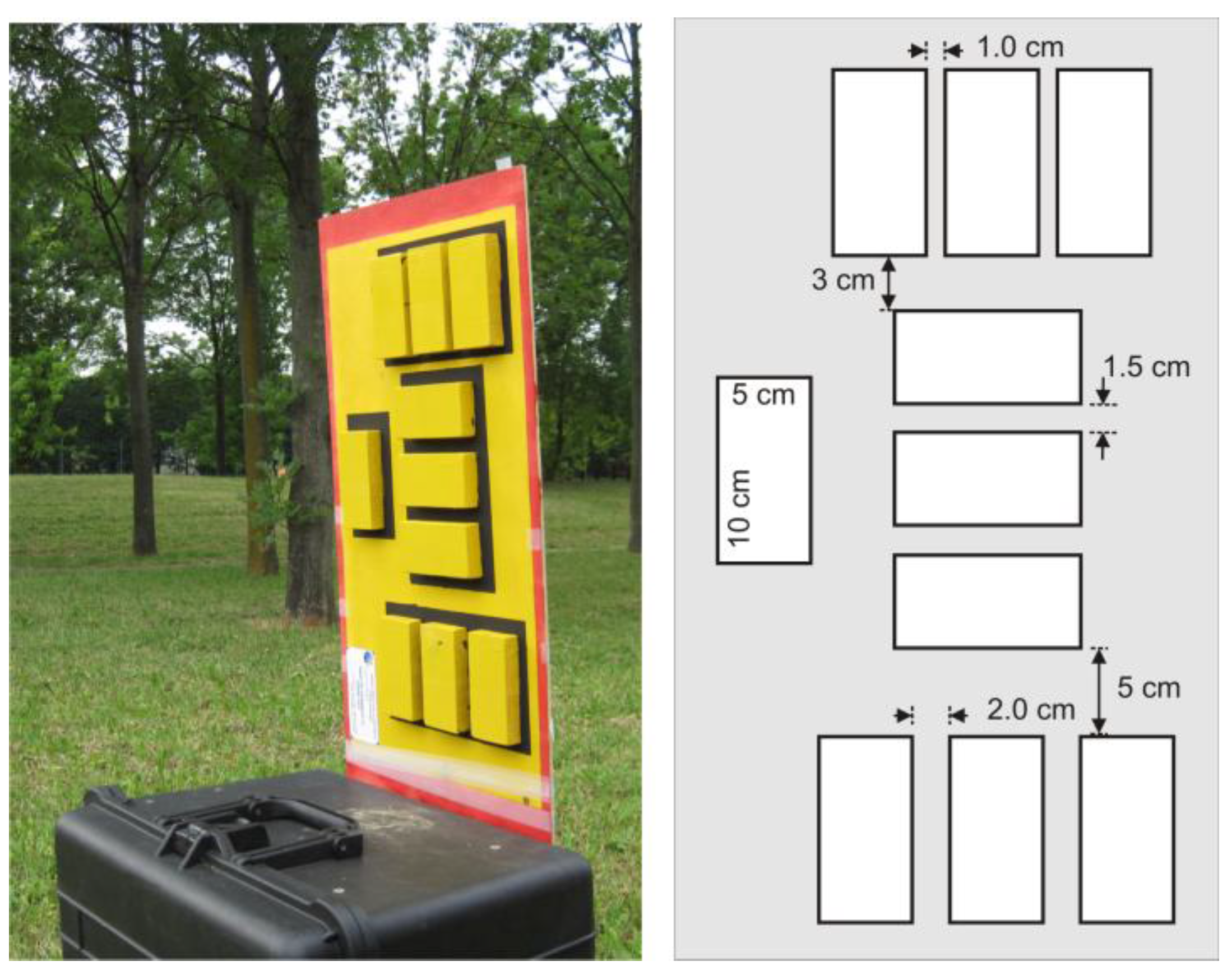
This paper presents the results of both numerical simulations and observations aimed to the optimization of a TLS survey at typical acquisition distances in architectural and cultural heritage application of TLS technique, i.e., up to about 100 m. In particular, an artificial target with differently spaced wood bricks has been scanned from 25 m, 50 m, 75 m and 100 m distance, the corresponding numerical simulations have been carried out and, finally, a brick wall and a historical building, with architectural details and a bust, have been observed. Besides the analysis of the obtained data, insights about the spot spacing necessary to obtain the required resolution (if achievable) in a general case are provided. This paper mainly focuses on evaluation of the sampling step necessary to obtain the required resolution. In this way, operational suggestions to the TLS practitioner are provided. An analysis of effects on the results of the material reflectance completes this study.

2. Laser Scanner Spatial Resolution

Two kinds of resolution can be defined for a TLS instrument: The range resolution, which accounts for its ability to differentiate two objects on the same LOS; and the angular resolution, which is the ability to distinguish two objects on adjacent LOSs. The first specification is governed by pulse length and typically is 3–4 mm for a long range instrument, whereas the second one depends on spatial sampling interval and laser beam width and should lead to a corresponding spatial resolution of ~10–15 mm at 50 m distance [4]. Besides these specifications, also the intensity resolution, i.e., the ability to differentiate adjacent areas, having similar but not equal reflectance, can be defined. In this paper the angular resolution, in particular the spatial resolution as a function of the acquisition distance, is the main topic.

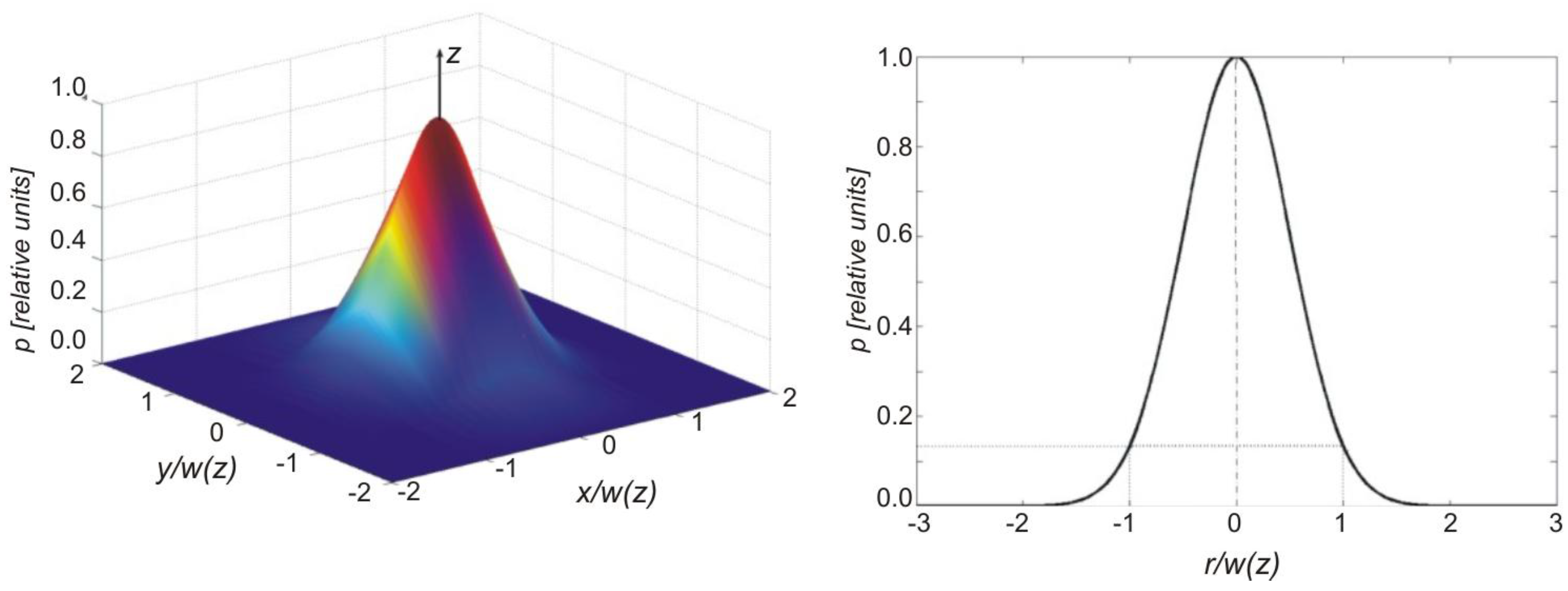
In order to maximize the localization performance of a laser rangefinder, in particular of a TLS instrument, the geometry of the laser resonator is such that a Gaussian beam is generated [9]. Figure 1 shows the power distribution of a Gaussian beam on a cross-section normal to the propagation direction. The beam diameter is commonly defined as the diameter that encircles 86% of the total beam power, that corresponds to e⁻² of the power axial value (with regard to the field amplitude, at the beam diameter it is e⁻¹ times the field axial value). Let w₀ be the waist of a Gaussian beam, i.e., the minimum spot diameter. For a range r and wavelength λ, the beam width is

$$w(r)=w_0\sqrt{1+{\left(\frac{\lambda r}{\pi {w_0}^2}\right)}^2}$$

(1)

Clearly, it is w₀ = w(0). The waist is related to the full divergence angle for the fundamental mode by

$$\Theta =\underset{r\to \infty }{\lim }\frac{2w(r)}{r}=\frac{2\lambda }{\pi w_0}=1.27\frac{\lambda }{2w_0}$$

(2)

Besides Θ, for a plane wave front incident upon a circular aperture of diameter D_F, which is the case in focusing optics, the full-cone angle of the central disc is defined:

$${\Theta }_p=2.44\frac{\lambda }{D_F}$$

(3)

This full-cone angle encircles about 84% of the total energy transmitted by the aperture. The angles Θ and Θ_p are very similar, but not equal, and are sometimes confused.

Figure 1. Power distribution around the laser beam axis (left panel), where z indicates the propagation direction, and radial power profile (right panel). The x, y and radial coordinates are normalized to the beam width w(z), that corresponds to exp(−2) of the power axial value.

Figure 1. Power distribution around the laser beam axis (left panel), where z indicates the propagation direction, and radial power profile (right panel). The x, y and radial coordinates are normalized to the beam width w(z), that corresponds to exp(−2) of the power axial value.

If $r$ is sufficiently large, which is the case for a long range TLS, a linear approximation of (1) can be used. For example, in the case of Optech ILRIS-3D instrument, it is

$$D(r)=1.7\times {10}^{-4}r+0.012$$

(4)

where both the spot diameter D(r) = 2w(r) and the range r are expressed in meters [7]. The constant is negligible for r larger than 300 m.

According to [4], a good measure of the angular resolution of the instrument can be the EIFOV, which can be computed taking into account the Average Modulation Transfer Functions (AMTFs), see [10], related to: (i) laser beam width; (ii) spatial sampling; (iii) quantization effects, (iv) focusing optics, where the latter in general can have negligible effects if the diameter of the optics is larger than the beam width. In general, the Modulation Transfer Function (MTF) is the magnitude of the Fourier transform of the point spread function and therefore is able to account for the response of an imaging system to an infinitesimal source of light. An AMTF is the spatially averaged MTF by assuming adequate probability density distributions of the independent variables, in this case the angular coordinates of a spherical reference frame. The AMTF of the whole system is the product of the component AMTFs (note that the variables in the Fourier space are spatial frequencies). Finally, the EIFOV is the length that corresponds to the cut-off spatial frequency threshold, i.e., the frequency for which the whole system AMTF is 2/π. To obtain a reliable EIFOV, reasonable hypotheses on the component AMTFs are necessary. With this very interesting approach, the authors obtained a resolution of 17.7 mm at 50 m for the ILRIS-3D instrument. Nevertheless, the practice of this instrument shows that 17.7 mm seems to be a too pessimistic value and that a ~10 mm value seems to be a better estimate for the instrumental resolution at 50 m distance if an adequate spatial sampling is used. Such a discrepancy could be related to the modeling of the beam width’s AMTF, where a uniform probability density function was assumed instead of a Gaussian one.

The EIFOV estimation is not in the scope of this paper, where the resolution is evaluated by means of numerical simulations and observation of an artificial target. The main aim of the paper is instead to search for a way to optimize the sampling step. Note that in all the studied cases, the observations are simulated or performed in normal incidence. If the incidence is not normal, the corresponding effects must be taken into account (e.g., elliptical spot instead of circular spot).

3. Numerical Simulations

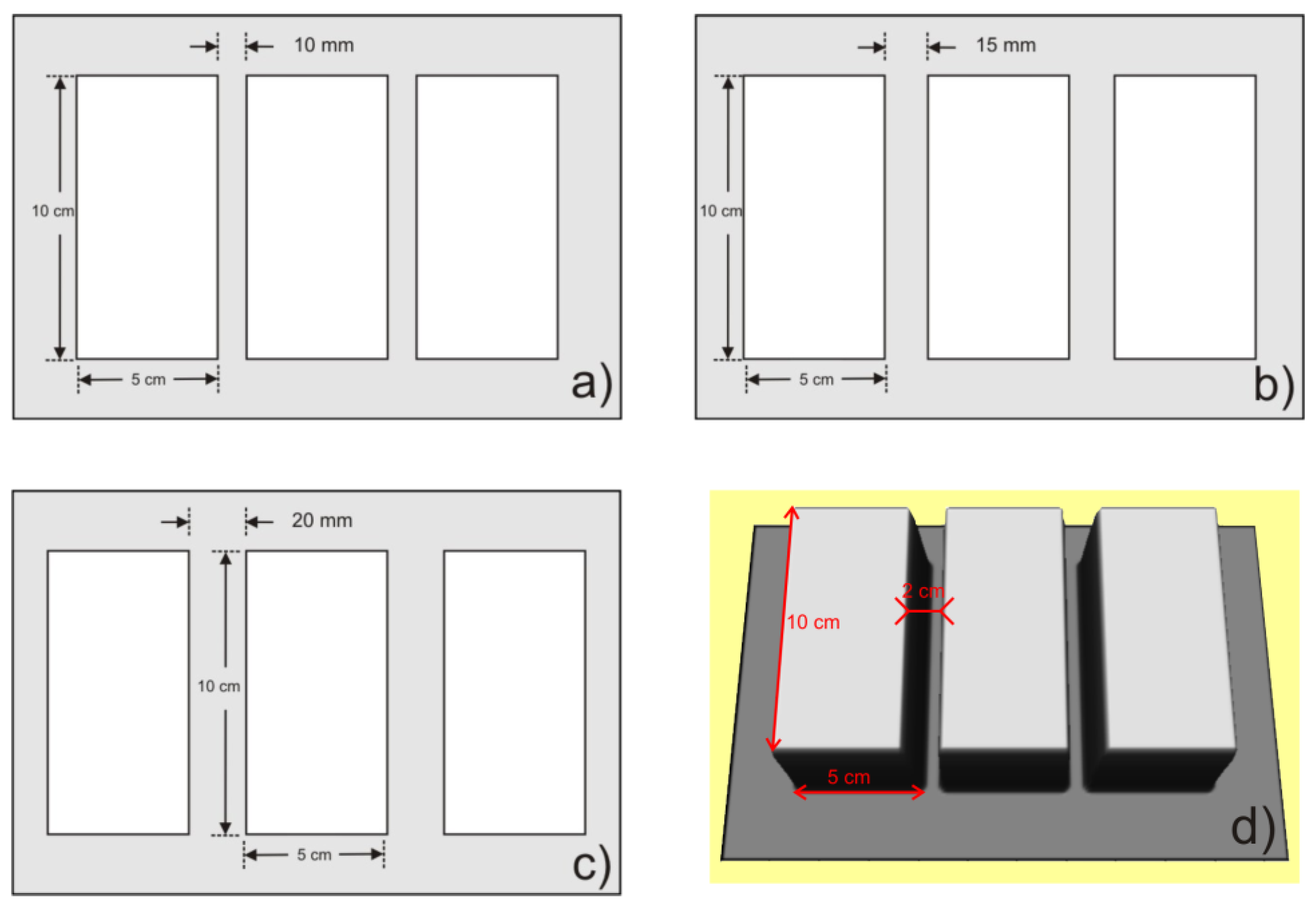
In order to evaluate the effects of sub-sampling and beam width, several series of numerical simulations have been carried out by defining virtual bricks having different spacing. As in the case of the artificial target described in Section 4, each simulated brick has 100 mm length, 50 mm high and 18 mm visible width with respect to the cement joint, and three systems of parallel bricks are modeled, with 10 mm, 15 mm and 20 mm spacing respectively (Figure 2). As in the experiments described in Section 4, the simulations are related to 25 m, 50 m, 75 m and 100 m acquisition distances. To carry out the numerical simulations, it is necessary to model: (a) the geometry of the objects, and (b) the TLS-based observation of these objects. The calculations are performed in MATLAB environment.

The geometry of each system of bricks is represented by a 2.5D elevation model z_hk = z(x_h,y_k), where x_h and y_k are defined on a regular grid with 0.1 mm spacing and whose plane is parallel to the simulated wall (Figure 2). The indices h and k vary from 1 to N_x and N_y respectively, depending on the system size. For example, if the three bricks are 10 mm spaced and simulated together with a 30 mm edge around them, it is N_x = 2300 and N_y = 1600. This grid size is 1–2 orders of magnitude lower than the simulated sampling step (the minimum ss taken into account in the simulations is 1 mm), spot size (the minimum spot size is 16.3 mm, that corresponds to 25 m acquisition distance) and brick spacing (the minimum value is 10 mm). For this reason, according to the Nyquist-Shannon sampling theorem [8], such a grid does not affect the results and therefore is reasonable.

Figure 2. Three synthetic targets related to: (a) 10 mm, (b) 15 mm, and (c) 20 mm brick spacing respectively. (d) 3D view of the 20 mm spaced bricks case.

Figure 2. Three synthetic targets related to: (a) 10 mm, (b) 15 mm, and (c) 20 mm brick spacing respectively. (d) 3D view of the 20 mm spaced bricks case.

The TLS acquisitions are modeled according to the technical specifications of ILRIS-3D instrument (Table 1) by means of: (i) Generation of Gaussian noise to model the error of the TLS’ rangefinder unit; (ii) Introduction of a Gaussian filter to model the effect of the power distribution of the laser beam; (iii) Decimation of the obtained points to model the spatial sampling.

Table 1. Optech ILRIS-3D main technical specifications.

Parameter	Value		Unit	Condition
Wavelength	1,535 (infrared)		nm	-
Laser class	1M			-
Pulse repetition frequency	2.5 a		kHz	-
Field of view	40 × 40 b		°	-
Minimum range	3 c		m	-
Maximum range	1,500		m	80% target reflectivity
	800	m		20% target reflectivity
	350	m		4% target reflectivity
Rangefinder unit accuracy	7		mm	100 m distance
Rangefinder unit resolution	4		mm	100 m distance
Laser beam divergence	0.17 d		mrad	-
Spot diameter	20.5		mm	100 m distance
Single point accuracy	8		mm	100 m distance
Modeling accuracy	3		mm	100 m distance
Minimum angular spot spacing	0.02		mrad	-
Minimum spot spacing	2		mm	100 m distance

^a A version with 10-kHz pulse repetition frequency is available;^b The field of view can be extended to 110° × 360° by using of a rotating/tilting head; ^c To obtain reliable radiometric information, the minimum range is about 15 m, see [12]. The geometric information is good even if the range is lower than 15 m; ^d Long range divergence, see Equation (2).

Table 1. Optech ILRIS-3D main technical specifications.

Parameter	Value		Unit	Condition
Wavelength	1,535 (infrared)		nm	-
Laser class	1M			-
Pulse repetition frequency	2.5 a		kHz	-
Field of view	40 × 40 b		°	-
Minimum range	3 c		m	-
Maximum range	1,500		m	80% target reflectivity
	800	m		20% target reflectivity
	350	m		4% target reflectivity
Rangefinder unit accuracy	7		mm	100 m distance
Rangefinder unit resolution	4		mm	100 m distance
Laser beam divergence	0.17 d		mrad	-
Spot diameter	20.5		mm	100 m distance
Single point accuracy	8		mm	100 m distance
Modeling accuracy	3		mm	100 m distance
Minimum angular spot spacing	0.02		mrad	-
Minimum spot spacing	2		mm	100 m distance

^a A version with 10-kHz pulse repetition frequency is available;^b The field of view can be extended to 110° × 360° by using of a rotating/tilting head; ^c To obtain reliable radiometric information, the minimum range is about 15 m, see [12]. The geometric information is good even if the range is lower than 15 m; ^d Long range divergence, see Equation (2).

The effect of the uncertainties, due to the rangefinder unit, is modeled by means of Gaussian noise with 5 mm standard deviation (SD). The elevation of the hk^th point therefore is z_nhk = z_hk + n_hk), where n_hk is a random entry coming from the probability density function

$$G_{z_{hk},\sigma }(z)=\frac{1}{\sqrt{2\pi }\sigma }\exp \left(-\frac{{(z-z_{hk})}^2}{2{\sigma }^2}\right)$$

(5)

i.e., the Gaussian centered at z_hk with SD σ = 5 mm. The chosen SD comes from both the ILRIS-3D technical specifications and the comparison between the results of numerical simulations and observations of the artificial target.

As stated above, the power distribution of a TLS laser beam generally has Gaussian profile. In the case of ILRIS-3D instrument, this fact is also confirmed by [11]. For each point (x_h,y_k,z_nhk), a Gaussian filter with standard deviation equal to the beam radius, i.e., $D/2$ with reference to Equation (4), is therefore introduced to blur the model. The filter equation for the hk^th point is

$$G_{(x_h,y_k),D/2}(x,y)=\frac{2}{\pi D^2}\exp \left(-\frac{2[{(x-x_h)}^2+{(y-y_k)}^2]}{D^2}\right)$$

(6)

and is used to obtain the blurred elevation z_bhk by means of the equation

$$z_{bhk}={\displaystyle \sum _{i=h-N_b}^{h+N_b}{\displaystyle \sum _{j=k-N_b}^{k+N_b}{G}_{(x_h,y_k),D/2}(x_i,y_j)}}{z}_{nhk}$$

(7)

where N_b = 3D/(2gs), with gs = 0.1 mm (reference grid spacing). In other words, the weighted averages in Equation (7) are computed within three SDs and, in this way, the fact that all the points within the spot concur to the pulse reflection is taken into account. Equation (7) is implemented in MATLAB in a very efficient way by means of the ‘fspecial’ function that performs the 2D special filtering.

Finally, the points of the noised and filtered model are decimated in order to simulate the spatial sampling of a TLS instrument. In these calculations the sampling steps 1 mm, 2 mm, etc., up to 20 mm are used. For each acquisition distance, 20 simulations are therefore carried out. The model is very simple, but the technical data provided by the instrument manufacturer do not allow a more sophisticated modeling.

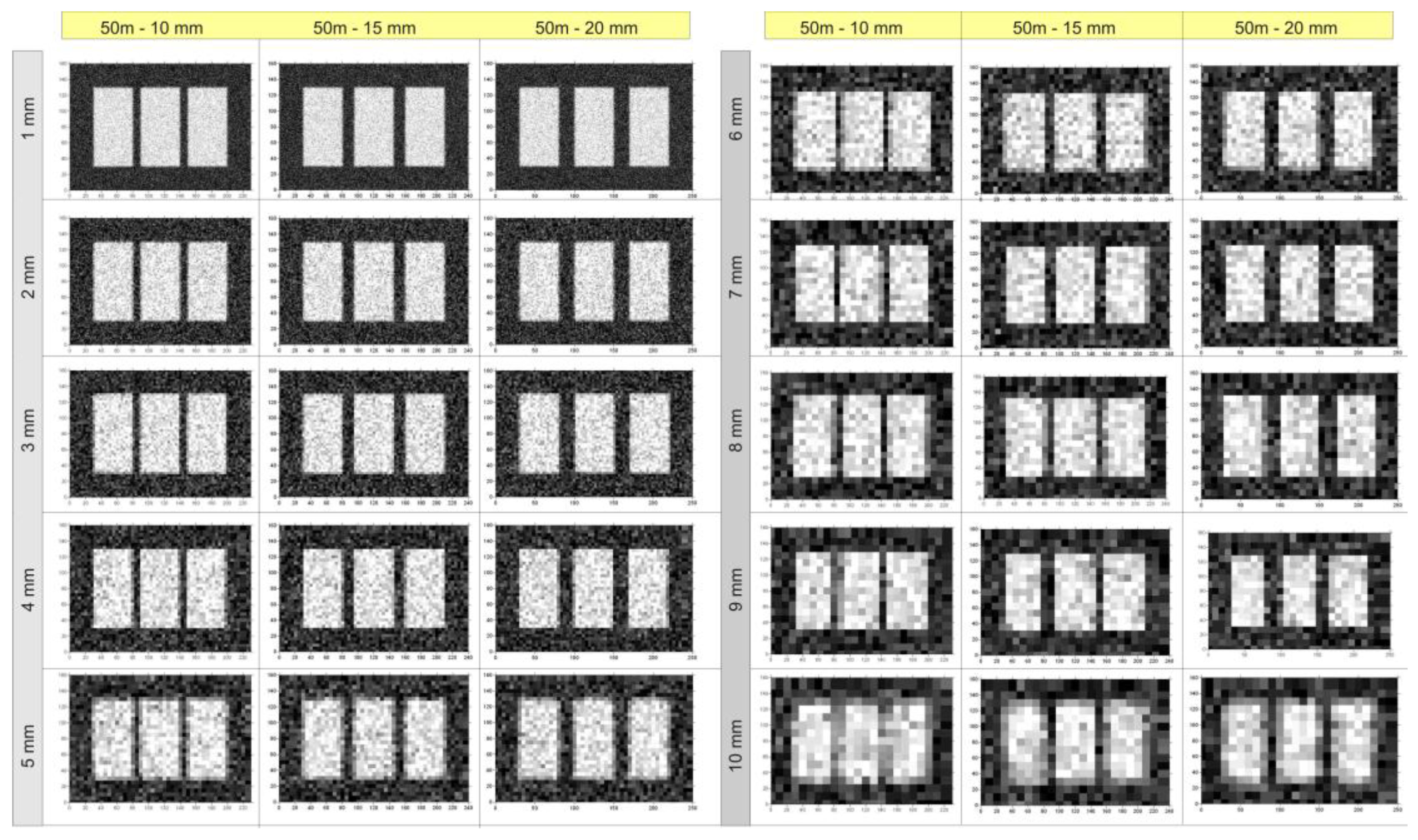
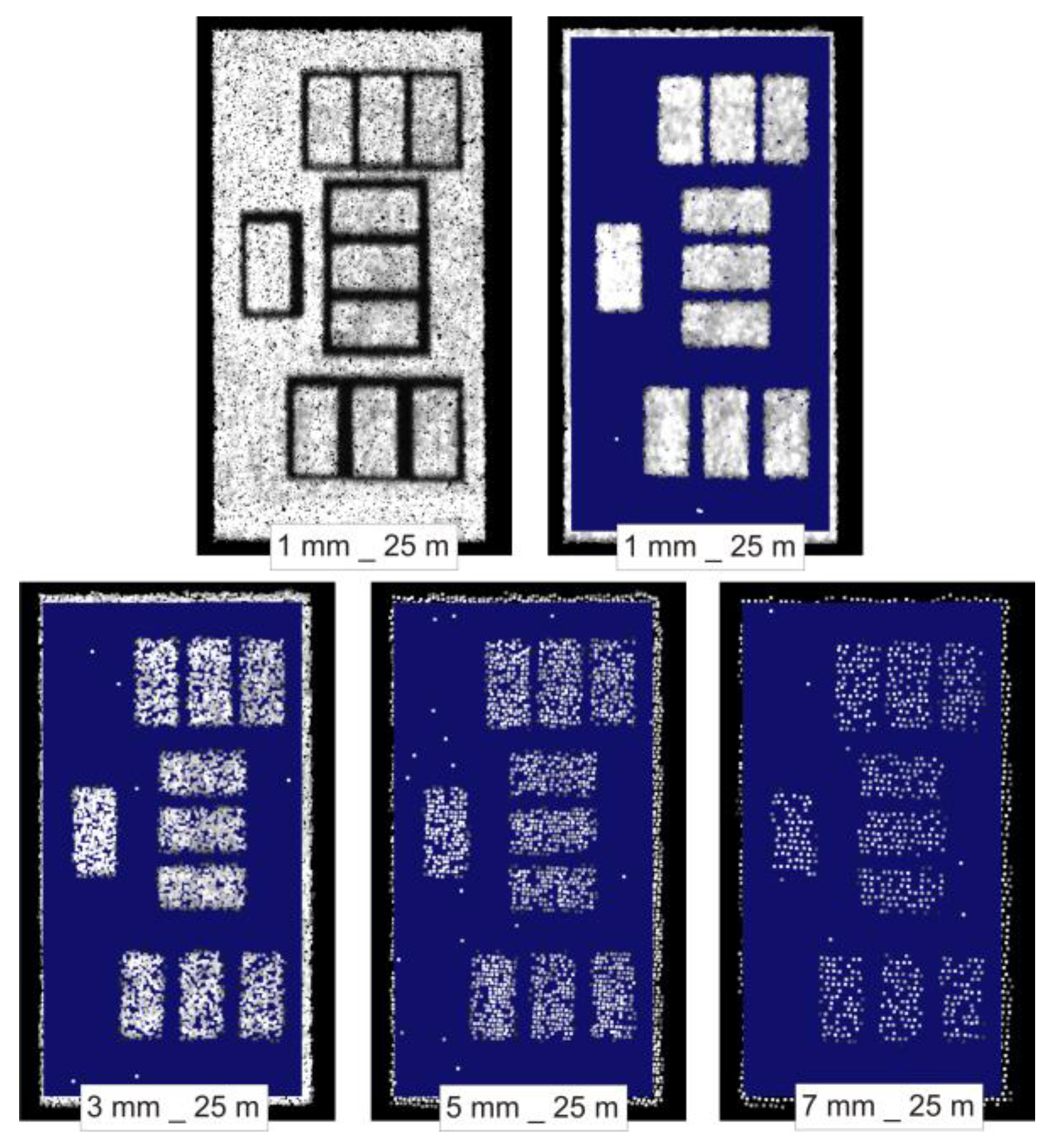
The results for some selected cases are shown in Figure 3, and the main results are summarized in Table 2. In this table, in particular, the cases where two different bricks can be easily recognized as distinct objects are shown together with the cases where the recognition is very difficult (borderline cases, corresponding to object spacing like the spatial resolution) and the ones where no recognition as a distinct object can be performed because the object spacing is below the spatial resolution. If a typical notebook with a 32 bit operating system is used, the simulation for an assigned acquisition distance is carried out in a few seconds, and all the results presented here can be obtained in a few minutes. This fact confirms that the 0.1 mm spacing for the reference matrix is a good choice.

Figure 3. Targets modeled from simulated point clouds at 50 m range. Besides the depicted case, the simulations at the 25 m, 75 m and 100 m modeled distances have been performed.

Figure 3. Targets modeled from simulated point clouds at 50 m range. Besides the depicted case, the simulations at the 25 m, 75 m and 100 m modeled distances have been performed.

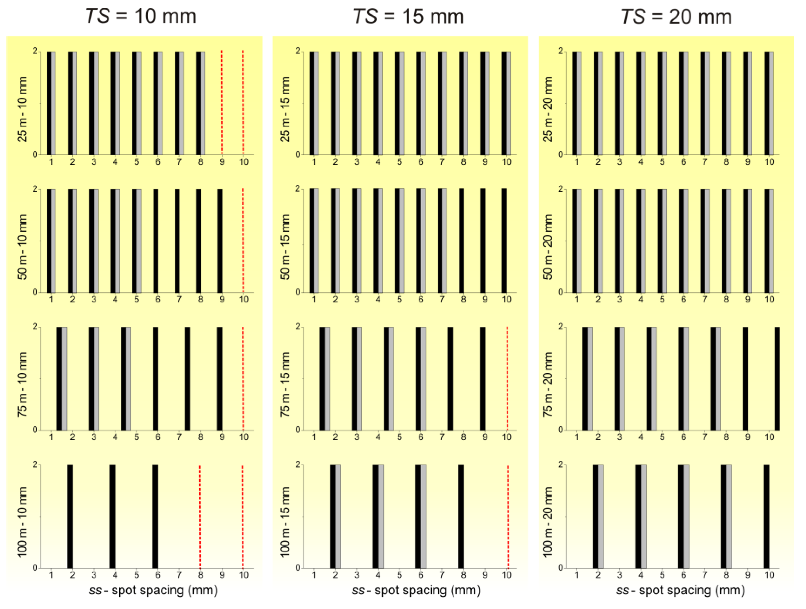
Table 2. Qualitative results of the target detection at 25, 50, 75 and 100 m. Legend: ss: spatial sampling; 2: recognition of two simulated bricks as distinct objects is easy; 1: borderline recognition cases, i.e., recognition difficult; 0: recognition not possible.

25 m distance—synthetic				50 m distance—synthetic
ss (mm)	Brick spacing (mm)			ss (mm)	Brick spacing (mm)
	10 mm	15 mm	20 mm		10 mm	15 mm	20 mm
1	2	2	2	1	2	2	2
2	2	2	2	2	2	2	2
3	2	2	2	3	2	2	2
4	2	2	2	4	2	2	2
5	2	2	2	5	2	2	2
6	2	2	2	6	2	2	2
7	2	2	2	7	1	2	2
8	1	2	2	8	1	1	2
9	0	1	2	9	1	1	1
10	0	1	1	10	0	1	1
75 m distance—synthetic				100 m distance—synthetic
ss (mm)	Brick spacing (mm)			ss (mm)	Brick spacing (mm)
	10 mm	15 mm	20 mm		10 mm	15 mm	20 mm
1.5	2	2	2	2	2	2	2
3	2	2	2	4	2	2	2
4.5	2	2	2	6	1	1	2
6	1	2	2	8	0	1	1
7.5	1	1	2	10	0	0	1
9	1	1	1
10.5	0	0	1

Table 2. Qualitative results of the target detection at 25, 50, 75 and 100 m. Legend: ss: spatial sampling; 2: recognition of two simulated bricks as distinct objects is easy; 1: borderline recognition cases, i.e., recognition difficult; 0: recognition not possible.

25 m distance—synthetic				50 m distance—synthetic
ss (mm)	Brick spacing (mm)			ss (mm)	Brick spacing (mm)
	10 mm	15 mm	20 mm		10 mm	15 mm	20 mm
1	2	2	2	1	2	2	2
2	2	2	2	2	2	2	2
3	2	2	2	3	2	2	2
4	2	2	2	4	2	2	2
5	2	2	2	5	2	2	2
6	2	2	2	6	2	2	2
7	2	2	2	7	1	2	2
8	1	2	2	8	1	1	2
9	0	1	2	9	1	1	1
10	0	1	1	10	0	1	1
75 m distance—synthetic				100 m distance—synthetic
ss (mm)	Brick spacing (mm)			ss (mm)	Brick spacing (mm)
	10 mm	15 mm	20 mm		10 mm	15 mm	20 mm
1.5	2	2	2	2	2	2	2
3	2	2	2	4	2	2	2
4.5	2	2	2	6	1	1	2
6	1	2	2	8	0	1	1
7.5	1	1	2	10	0	0	1
9	1	1	1
10.5	0	0	1

Since these simulations allow an evaluation of the effects on spatial resolution of changes in beam width and in spatial sampling, they can be used to simulate the behavior of an instrument on the basis of its technical specifications. In particular, the results could be used for choosing instrument type for a specific application. Finally, the MATLAB scripts developed to perform the numerical simulations can be requested from the authors, see contact information.

4. TLS Observations and Data Analysis

4.1. Artificial Target

The observations are carried out by using the Optech ILRIS-3D instrument, whose main technical specifications are summarized in Table 1. In order to allow an evaluation of the instrumental resolution in controlled conditions, an artificial target is used (Figure 4).

Figure 4. Artificial target for resolution testing.

Figure 4. Artificial target for resolution testing.

The artificial target is composed by 10 wood bricks, each one measuring 100 mm in length, 50 mm height and 18 mm visible width, placed on a wood panel that represents the plane of the cement joint. Three bricks are 10 mm spaced, three 15 mm spaced and, finally, another three are 20 mm spaced. In this way, the spatial resolution can be experimentally evaluated at several acquisition distances (here 25 m, 50 m, 75 m and 100 m) in conditions like the ones considered in the already described numerical simulations. Since the depths along the LOS of the acquired objects are significantly larger than the range resolution (18 mm compared with 3–4 mm), only effects related to the angular resolution are observed here. Figure 5 shows the 25 m range point clouds acquired with different settings for spot spacing. In particular, the acquisition with 7 mm sampling step still allows the recognition of target shapes but it is critical. The main qualitative results are summarized in Table 3.

Figure 5. Point clouds at 25 m range. The blue plane is parallel to the target and is used to highlight the shapes and details detection.

Figure 5. Point clouds at 25 m range. The blue plane is parallel to the target and is used to highlight the shapes and details detection.

Table 3. Qualitative results: ability for target shapes detection. Legend: ss: spatial sampling; 2: recognition of two simulated bricks as distinct objects is easy; 1: borderline recognition cases, i.e., recognition difficult; 0: recognition impossible.

25 m distance—real				50 m distance—real
ss (mm)	Brick spacing (mm)			ss (mm)	Brick spacing (mm)
	10 mm	15 mm	20 mm		10 mm	15 mm	20 mm
1	2	2	2	1	2	2	2
2	2	2	2	2	2	2	2
3	2	2	2	3	2	2	2
4	2	2	2	4	1	2	2
5	2	2	2	5	1	1	2
6	2	2	2	6	0	1	2
7	1	2	2	7	0	1	2
8	1	2	2	8	0	0	2
9	0	1	2	9	0	0	1
10	0	1	2	10	0	0	1
75 m distance—real				100 m distance—real
ss (mm)	Brick spacing (mm)			ss (mm)	Brick spacing (mm)
	10 mm	15 mm	20 mm		10 mm	15 mm	20 mm
1.5	2	2	2	2	0	2	2
3	2	2	2	4	0	2	2
4.5	2	2	2	6	0	1	2
6	1	2	2	8	0	0	1
7.5	0	1	2	10	0	0	0
9	0	0	1
10.5	0	0	0

Table 3. Qualitative results: ability for target shapes detection. Legend: ss: spatial sampling; 2: recognition of two simulated bricks as distinct objects is easy; 1: borderline recognition cases, i.e., recognition difficult; 0: recognition impossible.

25 m distance—real				50 m distance—real
ss (mm)	Brick spacing (mm)			ss (mm)	Brick spacing (mm)
	10 mm	15 mm	20 mm		10 mm	15 mm	20 mm
1	2	2	2	1	2	2	2
2	2	2	2	2	2	2	2
3	2	2	2	3	2	2	2
4	2	2	2	4	1	2	2
5	2	2	2	5	1	1	2
6	2	2	2	6	0	1	2
7	1	2	2	7	0	1	2
8	1	2	2	8	0	0	2
9	0	1	2	9	0	0	1
10	0	1	2	10	0	0	1
75 m distance—real				100 m distance—real
ss (mm)	Brick spacing (mm)			ss (mm)	Brick spacing (mm)
	10 mm	15 mm	20 mm		10 mm	15 mm	20 mm
1.5	2	2	2	2	0	2	2
3	2	2	2	4	0	2	2
4.5	2	2	2	6	0	1	2
6	1	2	2	8	0	0	1
7.5	0	1	2	10	0	0	0
9	0	0	1
10.5	0	0	0

Results are listed and normalized in Table 4, where the maximum spatial sampling (ss, in mm) for which the target separation (TS, in mm) can be observed is provided together with the corresponding ss/TS ratio. For each acquisition range, a maximum ss/TS value is therefore available in order to correctly settle the sampling step to achieve the required resolution. Since range r and spot diameter D are correlated as in Equation (4), the ss/TS ratios can also be considered as functions of D. These ss/TS values are provided based on the 25 m, 50 m, 75 m and 100 m acquisition ranges and for three target (bricks on the artificial target) separations, i.e., 10 mm, 15 mm and 20 mm. It is noteworthy that at 100 m range the achieved point cloud resolution is not good enough to allow the detection of the 10 mm gap between bricks, which is about a third of the spot divergence. For this reason and under the reasonable hypothesis of linear increase of the spot diameter with range, the assumption that the lower limit for details detection is one third of the laser beam is used later on.

Table 4. For each range r and the corresponding spot diameter D, the table shows the maximum sampling step (ss) that allows a correct separation between two targets whose spacing is TS, as well as the corresponding ss/TS ratio.

r (m)	D (mm)	ss (mm)			ss/TS
		10 mm	15 mm	20 mm
25	16.3	7	8	10	0.70	0.53	0.50
50	20.5	5	7	8	0.50	0.47	0.40
75	24.8	3	4.5	7.5	0.30	0.30	0.38
100	29.0	-	2	4	-	0.13	0.20

Table 4. For each range r and the corresponding spot diameter D, the table shows the maximum sampling step (ss) that allows a correct separation between two targets whose spacing is TS, as well as the corresponding ss/TS ratio.

r (m)	D (mm)	ss (mm)			ss/TS
		10 mm	15 mm	20 mm
25	16.3	7	8	10	0.70	0.53	0.50
50	20.5	5	7	8	0.50	0.47	0.40
75	24.8	3	4.5	7.5	0.30	0.30	0.38
100	29.0	-	2	4	-	0.13	0.20

Figure 6 shows the qualitative comparison between results from real and synthetic point clouds. The “2” and “0” values are used to test for success or failure respectively, according to the symbols used in Table 2 and Table 3. Good agreement is found, but the synthetic model appears in some cases to be too optimistic, while results from real data seem to be reasonable. At long distance, the relation between D and r should be linear, as shown by Equations (1) and (4), and non-linearity effects are improbable. The discrepancies therefore are probably due to the choice of the Gaussian window for the model blurring. Further investigations will be carried out to clarify this fact for distances over 100 m, to evaluate the tendency of the observed behavior. In any case, the operational indication for a TLS user whose choices are driven by the numerical simulations only, is that the set out ss should be about 30% lower than the one directly suggested by these simulations, if the acquisition distance is over 100 m and the wished resolution is ~2D/3. Moreover, the experimental results show that a resolution better than D/3 cannot be reached even if the simulations show that such a result is possible.

Figure 6. Black and gray columns represent the experiment’s success at defined range (r) and spot spacing (ss) using synthetic and real point clouds respectively. The red lines show complete failure.

Figure 6. Black and gray columns represent the experiment’s success at defined range (r) and spot spacing (ss) using synthetic and real point clouds respectively. The red lines show complete failure.

4.2. Resolution Estimation and Optimization of the Sampling Step

The ss/TS ratios are simply analyzed by means of a linear fit (Figure 7), showing a clear linear trend at the studied ranges. In this way, a simple empirical formula can be obtained in order to estimate the maximum sampling step that must be selected in order to ensure the desired resolution, under the conditions in which such a resolution can be effectively achieved ($TS>D/3$). A linear fit is

$$ss/TS=0.9-0.008r(TS>D/3)$$

(8)

where r is expressed in m. With this formula the sampling step can be chosen in order to allow the acquisition of all the desired geometric information by means of TLS acquisition at the range r with the minimum possible scanning times. The fact that the beam divergence, D, does not appear in Equation (8) should be noted. This formula is valid for the ILRIS-3D instrument only. However, the same experimental procedure can also be carried out in the case of other instruments, leading to the estimation of the zero and first order parameters of the equations that correspond to Equation (8).

Figure 7. Ratio between maximum sampling step (ss, in m) for which a target separation (TS, in m) can be achieved for 25 m, 50 m, 75 m and 100 m acquisition distance.

Figure 7. Ratio between maximum sampling step (ss, in m) for which a target separation (TS, in m) can be achieved for 25 m, 50 m, 75 m and 100 m acquisition distance.

The results obtained using the described experimentations, in particular the empirical Equation (8), which allow the creation of tabular values to easily define the most suitable ss for the specific application. For each range from 20 to 100 m and for three desired target separations, i.e., desired spatial resolutions, Table 5 reports the necessary maximum sampling step, expressed both in mm and in terms of the minimum sampling step of ILRIS-3D instrument. The cases where the desired resolution cannot be reached because it is similar or lower than a third of the beam width are also listed, while significant results are shown in bold.

Table 5. The EMPIR column provides the $ss/TS$ ratio obtained with Equation (5) at defined ranges r from 20 m to 100 m; D is the spot diameter; ss is the minimum achievable spot spacing with given r; TS is the target separation; max ss is the maximum spot spacing usable to detect the desired TS; and unit*ss is the corresponding number of spot spacing units in the case of ILRIS-3D instrument. The distances for which the desired resolution can be obtained (D > 3TS) are highlighted in bold. A column with 1/3 D is also shown because it is the lower limit for detection of small structures (see Section 4.1).

r (m)	D (mm)	ss (mm)	EMPIR	1/3 D (mm)	max ss (mm)	unit*ss	TS (mm)
20.0	15.40	0.40	0.74	5.1	4.4	11	6
30.0	17.10	0.60	0.66	5.7	4.0	7
40.0	18.80	0.80	0.58	6.3	3.5	4
50.0	20.50	1.00	0.50	6.8	3.0	3
60.0	22.20	1.20	0.42	7.4	2.5	2
70.0	23.90	1.40	0.34	8.0	2.0	1
80.0	25.60	1.60	0.26	8.5	1.6	1
90.0	27.30	1.80	0.18	9.1	1.1	1
100.0	29.00	2.00	0.10	9.7	0.6	-
20.0	15.40	0.40	0.74	5.1	5.2	13	7
30.0	17.10	0.60	0.66	5.7	4.6	8
40.0	18.80	0.80	0.58	6.3	4.1	5
50.0	20.50	1.00	0.50	6.8	3.5	4
60.0	22.20	1.20	0.42	7.4	2.9	2
70.0	23.90	1.40	0.34	8.0	2.4	2
80.0	25.60	1.60	0.26	8.5	1.8	1
90.0	27.30	1.80	0.18	9.1	1.3	1
100.0	29.00	2.00	0.10	9.7	0.7	-
20.0	15.40	0.40	0.74	5.1	7.4	19	10
30.0	17.10	0.60	0.66	5.7	6.6	11
40.0	18.80	0.80	0.58	6.3	5.8	7
50.0	20.50	1.00	0.50	6.8	5.0	5
60.0	22.20	1.20	0.42	7.4	4.2	4
70.0	23.90	1.40	0.34	8.0	3.4	2
80.0	25.60	1.60	0.26	8.5	2.6	2
90.0	27.30	1.80	0.18	9.1	1.8	1
100.0	29.00	2.00	0.10	9.7	1.0	1

Table 5. The EMPIR column provides the $ss/TS$ ratio obtained with Equation (5) at defined ranges r from 20 m to 100 m; D is the spot diameter; ss is the minimum achievable spot spacing with given r; TS is the target separation; max ss is the maximum spot spacing usable to detect the desired TS; and unit*ss is the corresponding number of spot spacing units in the case of ILRIS-3D instrument. The distances for which the desired resolution can be obtained (D > 3TS) are highlighted in bold. A column with 1/3 D is also shown because it is the lower limit for detection of small structures (see Section 4.1).

r (m)	D (mm)	ss (mm)	EMPIR	1/3 D (mm)	max ss (mm)	unit*ss	TS (mm)
20.0	15.40	0.40	0.74	5.1	4.4	11	6
30.0	17.10	0.60	0.66	5.7	4.0	7
40.0	18.80	0.80	0.58	6.3	3.5	4
50.0	20.50	1.00	0.50	6.8	3.0	3
60.0	22.20	1.20	0.42	7.4	2.5	2
70.0	23.90	1.40	0.34	8.0	2.0	1
80.0	25.60	1.60	0.26	8.5	1.6	1
90.0	27.30	1.80	0.18	9.1	1.1	1
100.0	29.00	2.00	0.10	9.7	0.6	-
20.0	15.40	0.40	0.74	5.1	5.2	13	7
30.0	17.10	0.60	0.66	5.7	4.6	8
40.0	18.80	0.80	0.58	6.3	4.1	5
50.0	20.50	1.00	0.50	6.8	3.5	4
60.0	22.20	1.20	0.42	7.4	2.9	2
70.0	23.90	1.40	0.34	8.0	2.4	2
80.0	25.60	1.60	0.26	8.5	1.8	1
90.0	27.30	1.80	0.18	9.1	1.3	1
100.0	29.00	2.00	0.10	9.7	0.7	-
20.0	15.40	0.40	0.74	5.1	7.4	19	10
30.0	17.10	0.60	0.66	5.7	6.6	11
40.0	18.80	0.80	0.58	6.3	5.8	7
50.0	20.50	1.00	0.50	6.8	5.0	5
60.0	22.20	1.20	0.42	7.4	4.2	4
70.0	23.90	1.40	0.34	8.0	3.4	2
80.0	25.60	1.60	0.26	8.5	2.6	2
90.0	27.30	1.80	0.18	9.1	1.8	1
100.0	29.00	2.00	0.10	9.7	1.0	1

4.3. Brick Wall

To validate the results obtained with the artificial target, the brick wall of a building is observed from about 35 m distance. Figure 8 shows a wall portion. The brick length varies from 130 mm to 260 mm, the mean brick height is 55 mm and the mean visible width, with respect to the mean plane of the cement joint is 5 mm (the SDs in height and width are 3 mm). The mean spacing between the bricks is 10 mm, with 3 mm SD. Using the empirical table (Table 5), and the reference range of about 40 m, the maximum spot spacing for an efficient acquisition of wall shapes (10 mm) results not larger than 5.8 mm, while the minimum detectable size is 6.3 mm. For this reason, the distance between bricks (10 mm) should be measurable.

Figure 8. Four point clouds acquired at about 35 m distance with different spot spacing. In particular, the last (7.6 mm) is not able to provide target shapes. The difference in gray level is due to different intensity of reflected pulses and has no effect on the geometric data.

Figure 8. Four point clouds acquired at about 35 m distance with different spot spacing. In particular, the last (7.6 mm) is not able to provide target shapes. The difference in gray level is due to different intensity of reflected pulses and has no effect on the geometric data.

Figure 8 shows the point clouds acquired on the wall portion of the house in front of the INGV office. A range of view is chosen and several scans are started, characterized by different spot spacing. The results highlight the ability of an efficient scanning up to the 5.8 threshold (i.e., 4.9 mm at about 35 m). Moreover, the fact that no good results can be obtained if a sampling step significantly larger than the threshold is settled should be noted, to confirm the validity of the proposed empirical method. Finally, image enhancement methods like those based on anisotropic diffusion could be used to further improve the results leading to a better resolution (e.g., [13,14]). Nevertheless, such a step is out of the scope of the present paper, which instead focuses on a fast method for TLS survey optimization.

4.4. Historic Building

The artificial target and the brick wall are both composed of parallel elements, the simulated and real bricks respectively. In these cases, the performance of a TLS instrument can be easily evaluated, but in the TLS practice simple shapes are not commonly observed. For this reason, investigations on TLS performance are generally carried out by using both simple and complex artificial targets, for example the 3D Siemensstern (see e.g., [15]).

In order to check the validity of the proposed optimization method in the case of a complex surface, characterized by relatively fine details, the front a historic building is observed from about 40 m. The typical size of the architectural details and busts that should be detected is 10 mm. The ss value, i.e., the maximum spatial sampling step that can be chosen in order to ensure the required resolution, is 5.8 mm in the case of parallel lines (Table 5).

Figure 9 and Figure 10 show the results (the upper part of a window of the building facade and a zoom of it respectively). The main results are: (i) no significant differences can be found if the sampling step is 2.4 mm (high oversampling case), 3.6 mm or 4.2 mm; (ii) a large amount of the details can be recognized if the sampling step is 5.4 mm; (iii) if the sampling step is 7.8 mm, some details are lost. The general validity of the method is confirmed, even though the fact that the results obtained in the case of parallel lines are slightly optimistic should be noted. In order to reliably use Table 5 in the case of general geometry, the ss values should be reduced by a factor of ~10%.

Figure 9. Details of a historic building observed from 40 m distance, with five different sampling steps.

Figure 9. Details of a historic building observed from 40 m distance, with five different sampling steps.

Figure 10. Details of a historic building observed from 40 m distance, with five different sampling steps. Details of the upper part of a window.

Figure 10. Details of a historic building observed from 40 m distance, with five different sampling steps. Details of the upper part of a window.

5. Discussion and Conclusions

The long range TLS instruments generally work at ranges from a couple of ten meters to some hundreds of meters, and are characterized by a laser beam whose diameter linearly increases along with the distance. The chosen spot spacing is generally smaller than the spot diameter providing a partial spot overlap. In the case of Optech ILRIS-3D, for example, a ratio between spot diameter (D) and spot spacing (ss) equal to 10 can be set. However, the actual resolution of a point cloud depends on both D and ss. Numerical modeling and experiments were carried out in order to study the ability of the ILRIS-3D instrument in surface shape details capturing for ranges lower than or equal to 100 m. The analyses described here were driven by the necessity of planning a series of TLS surveys in the city of Bologna, therefore for architectural survey and cultural heritage purposes. To carry out these surveys in an efficient way, a knowledge of the actual limitations imposed by ss and D on the target detection was very important. An approach to sampling step optimization in a TLS survey, aimed to reliably estimate the maximum sampling step that can be used to warrant the acquisition of a surface with the desired level of detail, was therefore developed. In other words, the aim was the computation of the optimal ratio between the sampling step and the desired resolution, since a larger sampling step with the same amount of information leads to less acquisition time.

The results show that the resolution estimates provided by [4] seem to be quite pessimistic. For example, at 50 m distance their estimate for ILRIS-3D instrument is 17.7 mm, but the experimental and numerical results obtained here show that a 10 mm interstice between two bricks can be easily acquired and modeled for such an acquisition distance. On the other hand, too optimistic affirmations can also be found, as in the case of [6], which identifies the resolution with the sampling step thanks to the correlated sampling, i.e., the sampling with overlapped laser spots. If a 0.9 mm sampling step is used at 50 m acquisition distance, i.e., the minimum possible ILRIS-3D spot spacing at such a distance, according to [6], this should lead to a point cloud with a similar resolution, but this is incorrect. The resolution is 10 mm instead and can be achieved by applying a 5.0 mm sampling step (ss/TS = 0.5). If the approach suggested by [6] is used, a larger amount of data is acquired in a time correspondingly 30 times higher, without any gain in the actual amount of acquired information.

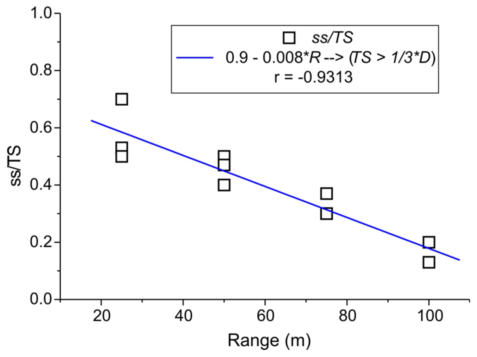
A very interesting result is that an empirical relation between the range and the ss/TS ratio exists, Equation (8). With this equation, or the corresponding Table 5, the user can settle the optimal sampling step, ss, for which a required object separation, TS, is obtained. The equation holds for ILRIS-3D instrument, but the proposed method can easily be applied to other instruments to obtain the corresponding empirical equations. The method has a general validity, since the physical processes involved in the TLS-based acquisition are the same for each time-of-flight instrument, but a data fit based on the specific characteristics of the used instrument is necessary. The comparison between the experimental data and the simulation results shows that from the beam width and the sampling step, and assuming reliable noise levels, a relatively accurate estimation of the spatial resolution as well as of the optimal ss/TS ratio can be carried out. In this way, a user can evaluate the required sampling step for the available instrument, or can choose between two or more instruments for a specific observation if they are available. The fact that the obtained empirical law is related to a simple geometry of the target should be noted. This is an ideal limit for surveying and therefore the corresponding ss/TS values are insuperable thresholds. 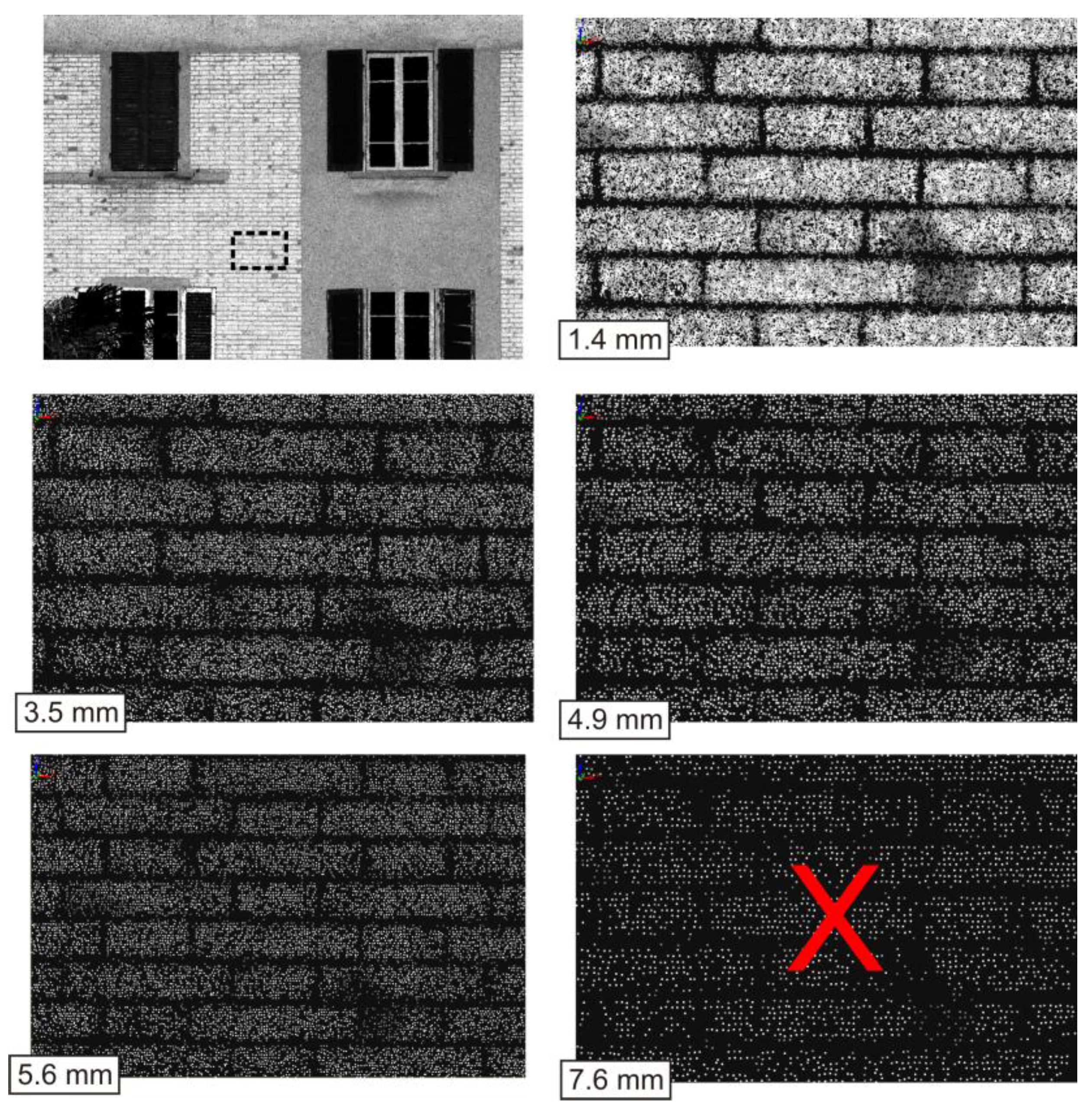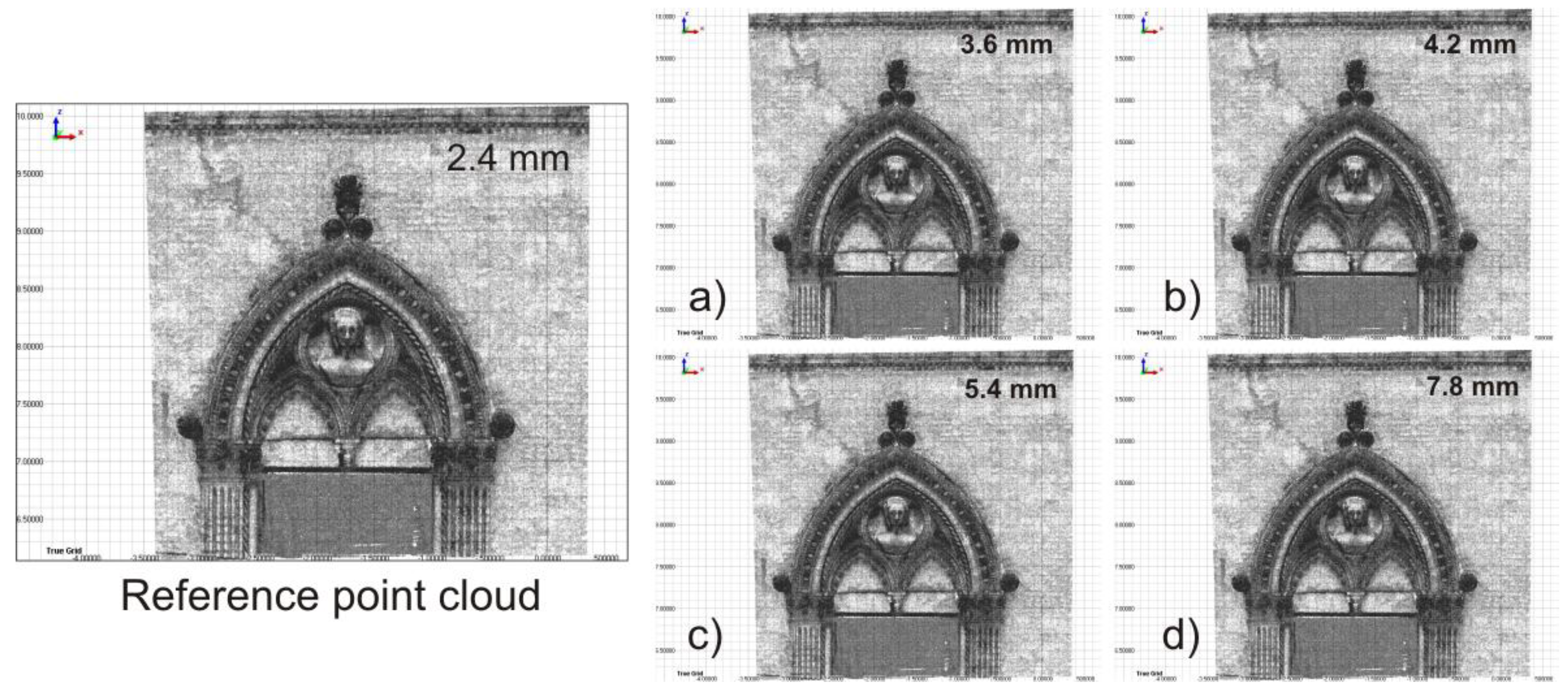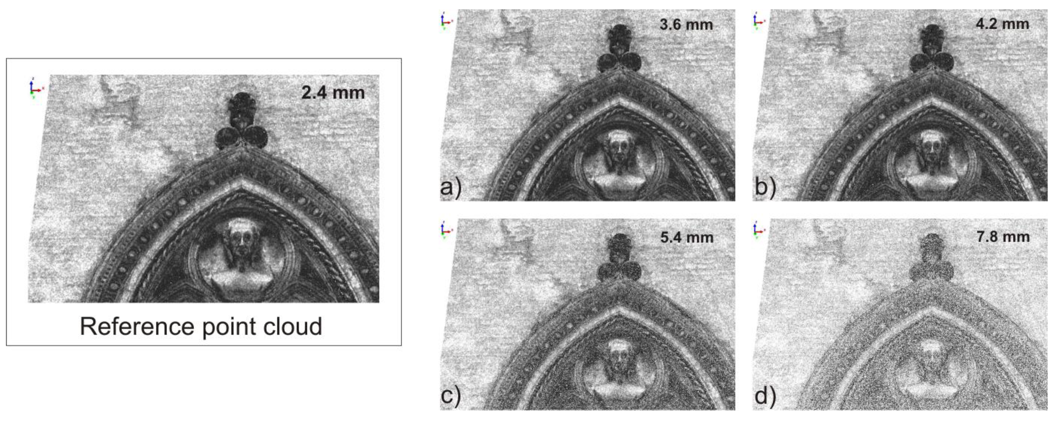If a ss/TS value larger than this threshold is set, surely the required resolution is not achieved. Nevertheless, in the case of a complex surface, the sampling step should be ~10% shorter than the threshold, as shown in the case of the historical building observation.

The experiments and the numerical simulations deal with acquisition distances up to 100 m, and the results could not be directly extrapolated to significantly longer distances. Other experiments, with artificial targets having different shapes and sizes, will be carried out in order to extend the results at distances up to one kilometer. Moreover, other experiments are planned to study the real relation between r and D for some commercially available long range TLS instruments.

The fact that the model resolution is beyond the scope of this paper should be noted. Although the final result of a TLS survey is sometimes a digital model, this study deals with instrumental performance, in particular spatial resolution, not with model resolution. If the modeling of sharp features like edges, thin tubes, wires and others is necessary, the obtained ss/TS values could be overestimated because a more adequate number of points would be required.