Optimizing Spatial Resolution of Imagery for Urban Form Detection—The Cases of France and Vietnam

Abstract

The multitude of satellite data products available offers a large choice for urban studies. Urban space is known for its high heterogeneity in structure, shape and materials. To approach this heterogeneity, finding the optimal spatial resolution (OSR) is needed for urban form detection from remote sensing imagery. By applying the local variance method to our datasets (pan-sharpened images), we can identify OSR at two levels of observation: individual urban elements and urban districts in two agglomerations in West Europe (Strasbourg, France) and in Southeast Asia (Da Nang, Vietnam). The OSR corresponds to the minimal variance of largest number of spectral bands. We carry out three categories of interval values of spatial resolutions for identifying OSR: from 0.8 m to 3 m for isolated objects, from 6 m to 8 m for vegetation area and equal or higher than 20 m for urban district. At the urban district level, according to spatial patterns, form, size and material of elements, we propose the range of OSR between 30 m and 40 m for detecting administrative districts, new residential districts and residential discontinuous districts. The detection of industrial districts refers to a coarser OSR from 50 m to 60 m. The residential continuous dense districts effectively need a finer OSR of between 20 m and 30 m for their optimal identification. We also use fractal dimensions to identify the threshold of homogeneity/heterogeneity of urban structure at urban district level. It seems therefore that our approaches are robust and transferable to different urban contexts.

1. Introduction

If today, almost 50% of the world’s population is urban, cities in developing countries are especially well-known for their rapid urbanization rate and their high concentration of population [1]. The rapid increases of urban settlements, the spontaneous growth of precarious habitations, as well as self-construction, are some consequences of non-regulatory urbanization processes, population migrations from poor or unsafe regions or non-appropriate planning provision regarding the strength of urban migration fluxes or natural growth rate. Consequently, monitoring and planning issues become an important challenge in developing countries.

In this situation, the capacity of urban planning in terms of mapping and map-updating process becomes an essential task. It requires accurate and up-to-date data in order to provide relevant information to manage human activities such as transport planning, urban cadastre and, more generally, environmental impact assessment or urban landscape studies in the long term. For several years, remotely sensed imageries represent a very significant data source in this context and provide homogeneous, regular, and up-to-date data to support all tasks of urban planning. They have been accepted as an operational tool for mapping, monitoring and modeling of environmental variables and processes. Especially for developing countries, remote sensing imagery offers a unique access to primary data about the status of land surfaces.

For an effective support to manage the territory, urban planners have to choose among a large variety of information sets, some extracted from remotely sensed imageries that provide specific information in terms of spatial, spectral and temporal resolutions [2,3]. High Spatial Resolution imagery sensors (HSR: from 30 to 3 m) allows analyzing urban areas on regional or metropolitan scales when Very High Spatial Resolution imagery ones (VHSR: 3 to 0.5 m) enable the analyses of urban fabric and the composition from urban blocks to individual elements (house, tree, road, etc.). These new VHSR images meet the needs of geographical information from 1:100,000 to 1:10,000 which are the scales used in regional and urban planning [2,4,5].

For urban purposes, spatial resolutions have important implications because the most relevant criteria is the choice of images adapted to final products. Indeed, cities are characterized by a high heterogeneity of materials and urban objects in terms of size, forms and urban fabric morphology. This heterogeneity becomes very important in the case of cities in developing countries because of self-construction processes [6]. For an optimal quantitative analysis in urban studies, the choice of an adapted spatial resolution to identify automatically geographical objects is still a difficult task. The optimal pixel size is influenced by the spatial structure of the investigated objects and the image processing designs, e.g., spectral classification, regression, texture analysis [7]. The spatial characteristics of the studied object must therefore be targeted before an optimal resolution can be chosen.

In this paper, the objective is therefore to apply the concept of Optimal Spatial Resolution (OSR) initially used in forest areas [8] and detailed in the next section (Section 2.1) for urban form detection. We suggest that it is possible to define relationships between urban objects on ground at two levels (urban element and urban district) and spatial resolution of remotely sensed images. The aim here is to define objects of interest at these two levels of observation and their corresponding optimal spatial resolution range for various urban objects. Two cities with typical urban forms of (1) West Europe; and (2) Southeast Asia are used as test sites. The main hypothesis is that the methods used may be transferred through different scales of study and through various types of city. The definition of the concept of OSR is followed by related works searching to identify an adapted spatial resolution to the different scales of analyses (Section 2.2). Study sites and datasets are then presented in Section 3. The proposed method to identify OSR at two levels of observation is detailed in Section 4. Finally, some results are discussed in Section 5. Especially, in Section 6, we also use fractal dimensions to characterize, in a complementary way, urban structure of districts in order to observe the threshold of homogeneity/heterogeneity of spatial organization by changing pixel size. According to [9,10,11,12,13,14,15,16], the identification of these fractal urban structures is based on the textural information of images (spatial organization of grey levels) by the homogeneity criteria. We hypothesize that the OSR or the range of OSR is, at the same time, the threshold of homogeneity at which spatial organization of built-up and vegetation has the best representation and thus reaches the highest values of fractal dimensions. So in this section, we examine: (1) how the threshold of homogeneity/heterogeneity of urban structure through fractal dimensions evolves by changing pixel size; and (2) the possible link between the fractal dimensions of such threshold of homogeneity/heterogeneity and the OSR result? The conclusion and perspectives are developed at the end of paper.

2. Background

2.1. The Concept of Optimal Spatial Resolution (OSR)

The problem of definition of geographical objects is complex because it refers to various spatial entities formed by numerous elements distributed within a continuum, the geographic area. For example, in the case of urban areas, a residential urban district consists of an aggregate of individual houses with various sizes, separated by green spaces and road networks. In order to identify this geographical object from remotely sensed imagery, relevant questions are: how many houses are necessary to define an urban district? What are the typical size and shape of the houses? What is the maximum distance between houses to differentiate this urban district? The simple example shows that the definition of any geographical entity (an urban district, a forest, etc.) is the result of a spatial sampling where some features are considered as relevant components while others appear as negligible.

From this reasoning, a formal definition of a geographical entity proposed by [8] is exposed: “A geographical entity is an earth surface feature assemblage characterized by a given scale and spatial aggregation level”. Then a fundamental question to answer is: What is the number and size of spatial sampling units that should be used to divide a geographic area in order to provide the “most” representative observations about the entities under investigation? Marceau et al. [8] also proposed the definition of an OSR that can be defined as the “spatial sampling grid corresponding to the scale and aggregation level characteristic of the geographical entity of interest”.

The existence of multiple sensors with different spatial resolutions seems to be advantageous for the choice of data sources, the objectives of determination and the scale of research for urban environment studies, but this one strengthens also the need of clear and operational definitions. The scale of measurement using remote sensing data is determined by the size of pixel or more precisely the spatial resolution of an image (or sensor’s Instantaneous field of view (IFOV) [17]). In this paper, we search an optimal spatial resolution in order to identify any urban elementary object. As such, spatial resolution plays an important role for products interpretation [18,19]. Woodcock and Strahler [19] suggest that an appropriate scale for observation is a function of the type of environment and the kind of information desired. The choice of scale is therefore determined by the size of the studied area and the type of phenomena analyzed.

Since the early 1980s, the first HSR images, Openshaw [20] showed that one of the fundamental problems of studying aggregated data is the dependence of results on the unit surfaces studied (Modifiable Aerial Unit Problem, MAUP). A phenomenon that appears homogeneous at small scale may become heterogeneous at larger scale. Extrapolating the results of one scale to another may lead to errors of interpretation, especially when the heterogeneity predominates [21,22]. Grégoire et al. [23] specify that the homogeneity of a scale of measurement is relative to a particular size. The homogeneity, based on the comparison between adjacent zones according to their content, depends on all geographical objects which the user searches to apprehend. Welch [24] completed this reasoning by defining the minimum size of pixels in order to identify the different urban land use patterns.

Nijland et al. [7,8,19,25,26,27,28,29,30,31] approached the spatial resolution to extract land use from satellite imagery. Nijland et al. [7,25] used the variogram method for characterizing spatial variation of imagery by calculating it as half the average squared distance between the paired data values. Introducing the local variance or the average local variance (ALV) as a function of spatial resolution for measuring spatial structure, Nijland et al. [7,8,19,26,27,28,29,30,31] showed that there is no unique spatial resolution appropriate for identifying and analyzing various urban features. The study of spatial structure of images is a function of the relation between the size of objects in the scene and spatial resolution. Woodcock et al. [19] considered that if the spatial resolution is considerably finer than the objects in the scene, most of the measurements in the image will be highly correlated with their neighbors and a measure of local variance will be low. If the objects approximate the size of resolution of pixels, then the likelihood of neighbors being similar decreases and the local variance rises. As the size of the resolution of pixels increase and many objects are found in a single resolution of pixel, the local variance decreases.

The appearance of VHSR images in the late 1990s has modified the territory vision because urban geographical objects classically identified from air photos become identifiable also from these remotely sensed imageries. The per-pixel classification becomes more and more inappropriate in urban context [32]. Indeed, the spectral measurements collected from an image are not independent from the sampling methods used. In this case, these VHRS images are to support classification methods considering geographical objects to identify adequate resolutions for their extraction. A relevant question in actual context is “What is the OSR adapted to, to identify and analyze geographical objects in a multi-scale approach of urban areas? May the methods used for a scale be applied to another through the change of spatial organization of elementary urban objects at each scale?”

2.2. Related Works to Identify ‘OSR’ on Urban Environment

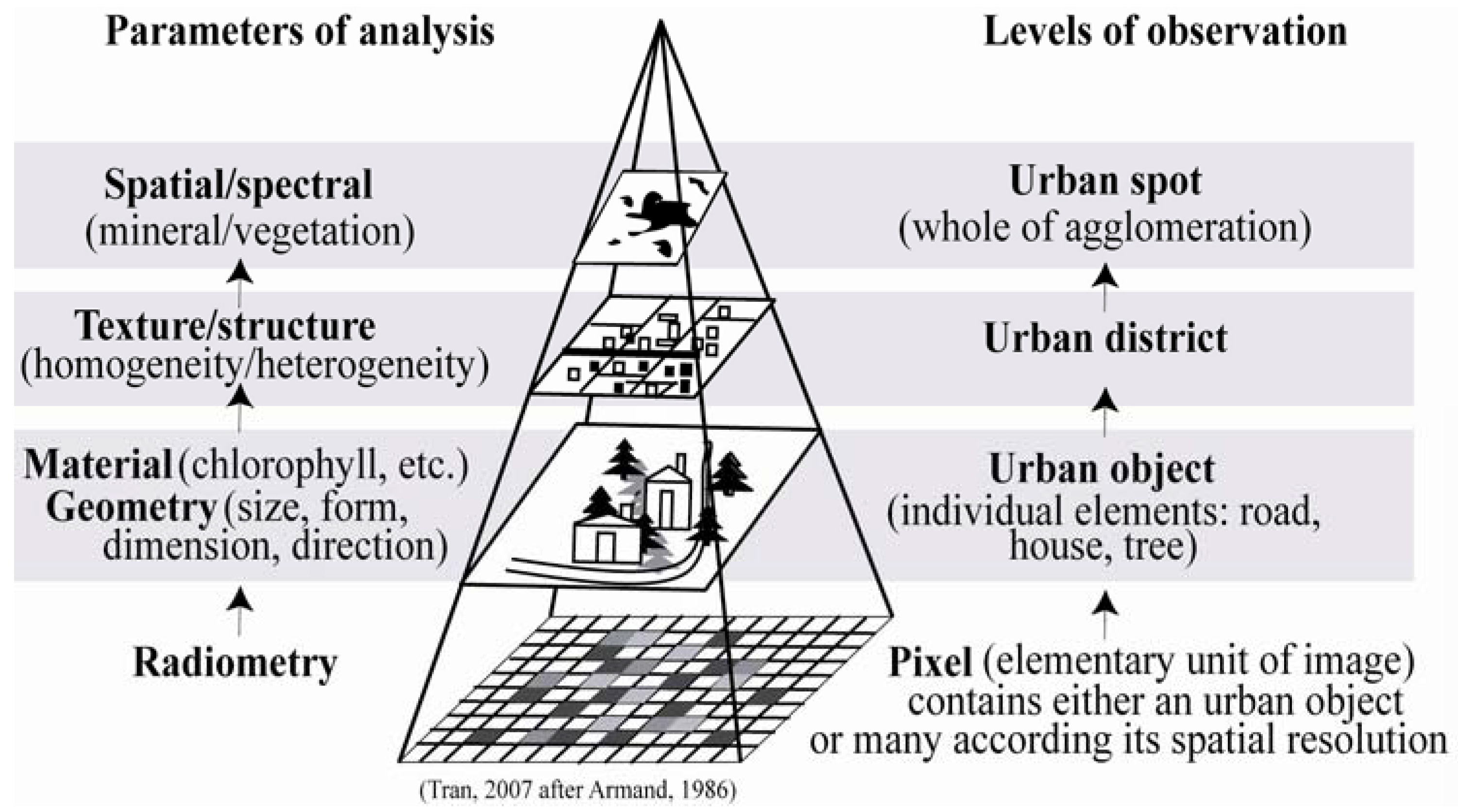
In urban planning and management, three levels of observation are commonly used (Figure 1): (1) the level of the urban spot or urban area (agglomeration) allowing to distinguish mineral from natural spaces; (2) the level of urban district characterized by several urban fabric patterns; and (3) the level of urban objects composed of basic element (building, tree, road, etc.). For each level of observation, related works based on remotely sensed imagery are remaindered.

Figure 1. Levels of observation in urban studies and parameters of analysis from remotely sensed imageries.

Figure 1. Levels of observation in urban studies and parameters of analysis from remotely sensed imageries.

At the level of urban area (urban spot), the concept of Urban Morphological Area is commonly used [33]. The extraction of urban area using remotely sensed data constitutes the distinction of built-up area from rural zone by separating mineral and vegetation spaces. Using the spatial frequencies (size and density), Armand [34] differentiated built-up area from rural area by its high spatial frequencies. This requires sensors with low or intermediate spatial resolution (such as Landsat MSS). These spatial resolutions are sufficient to define urban area [19,32].

At the level of urban district, basic elements are urban fabrics. This level allows observing different urban structures according to spatial distribution between built-up area and vegetation. The identification of these structures is based on the texture (spatial organization of grey levels) according to homogeneity criteria. For example, continuous and dense urban fabric is different to discontinuous ones by heterogeneous texture due to the varying size of constitutive objects and their various materials of construction. Using the contrast and the spatial frequencies of urban land use/cover classes as a factor which determines the spatial resolution requirements for detailed urban area analysis, Welch [24] suggested that if the assumption is correct that a minimum of four pixels is needed for reliable identification or classification of basic land parcels, an appropriate spatial resolution of 5 m would be required for an urban environment in Asia, whereas 30 m may be adequate for analysis of some urban areas in the United States. Using the same method, Armand [35] proposed adequate sensors to identify different urban fabrics in Bouake (Côte d’Ivoire or Ivory Coast). This means that: (1) a spatial resolution of 30 m (Landsat TM) is adapted to identify industrial and service sector patterns; (2) a spatial resolution of 20 m images is suitable to extract collective and residential urban fabric; (3) a spatial resolution of 10 m allows identifying low or high density of built-up urban fabric; and (4) a spatial resolution under five meters (VHRS) is adapted to extract spontaneous urban fabric. Moreover, focusing on the relationship between spatial resolution and urban reflectance, Small [3,36,37] used spatial self-correlation of image, which measures correlation degree between pixel size and its reflectance to estimate spatial variation of reflectance, in order to determine the adequate pixel size in the scene. He used a set of images with a one meter spatial resolution (panchromatic) on 6,357 sites of 14 urban areas characterized by different urban contexts in the world. He considered that the range of resolution from 10 m to 20 m is an adequate resolution to identify the reflectance of urban area for most urban areas except for Nanjing.

At the level of urban objects, all constitutive elements of urban block are then defined by their dimensions and shapes. This level allows analyzing the individual elements (building, tree, road, etc.). The extraction of these elements is based on the identification of both material (spectral response) and geometries (spatial response) characteristics of objects themselves. They may contain an urban object or many urban objects depending on the spatial resolution. The relevant spatial resolution or the adapted spatial resolution to identify and analyze an urban individual object remains to be defined.

Regarding these related works, we can assume that the OSR is not identical for all objects at the same level. The OSR at the range of 5 to 30 m spatial resolution (HSR images) generally corresponds to intra-urban analyses in developed countries because of coarse size of urban objects. We also assume that the identification of urban districts in developing countries often requires a higher OSR because of their small parcels, compact structures and the narrow street patterns. Moreover, the OSR seems to depend on urban context, geometric form of urban objects and spatial organization of urban areas. Therefore, these results cannot be directly applied on urban areas in developing countries due to their highly varying morphological characteristics. Indeed, these urban areas require their own OSR adapted for each type of agglomeration.

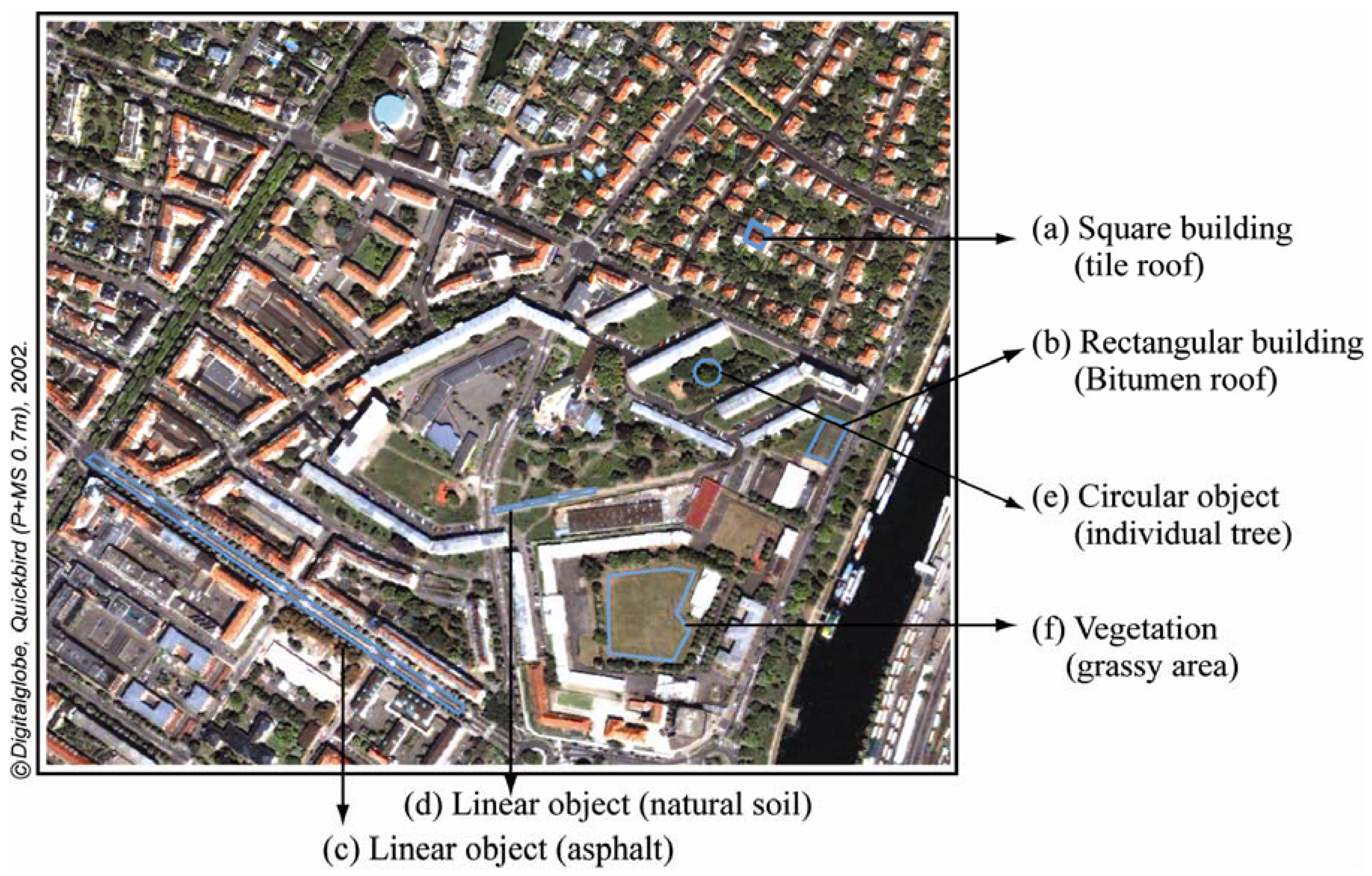
3. Study Site and Dataset

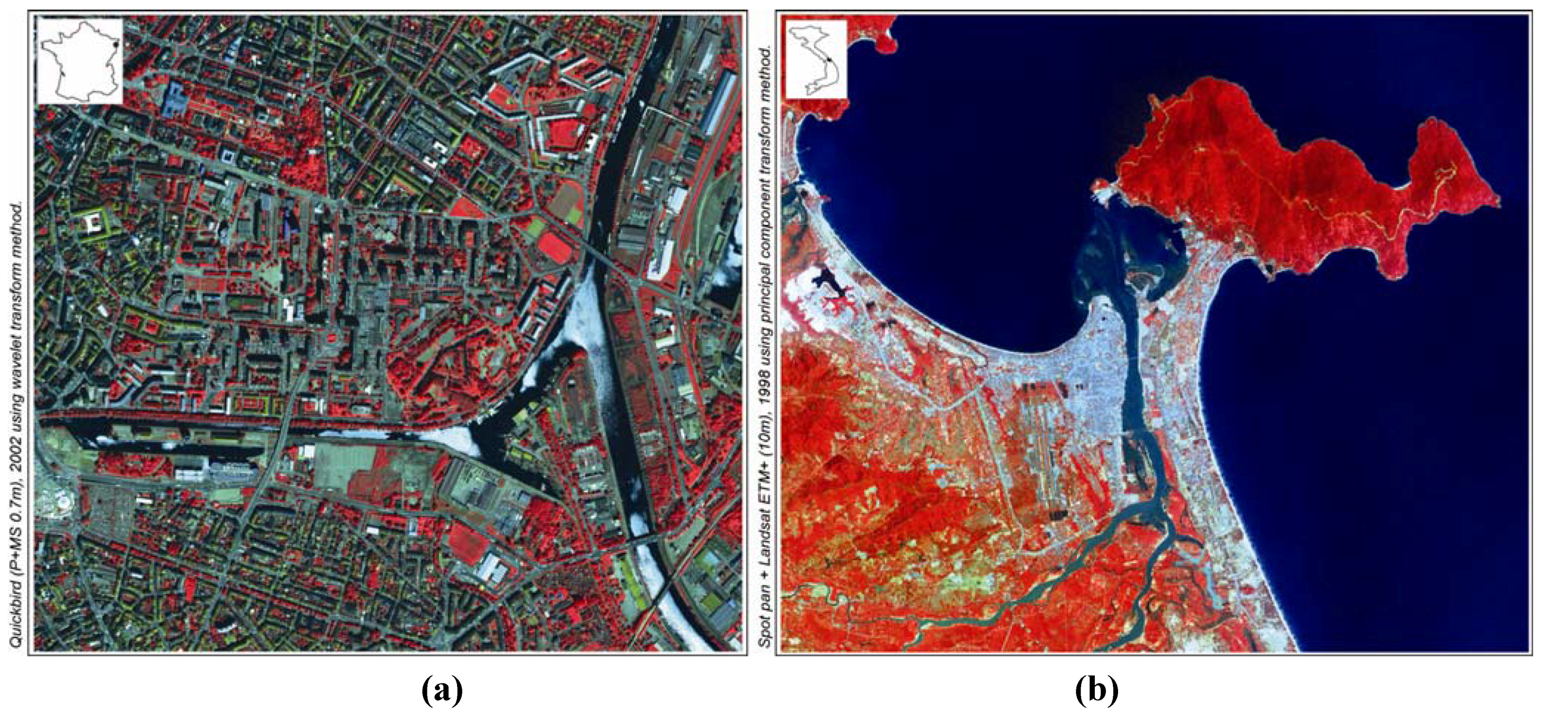
This study proceeds on two levels of observation: urban object and urban district. The test site for the urban object level analysis covers a large district on the East of Strasbourg (France). It contains all urban representative objects of the typical urban environment of West Europe (Strasbourg, France—Figure 2(a)). The study site for urban district level analysis covers the whole Da Nang city (Vietnam—Figure 2(b)). For the urban object level, a pan-sharpened of Quickbird image (©Digitalglobe, 2002) between its panchromatic band and its four spectral bands is used [38]. The fusion method is based on ARSIS concept which applies the wavelet transform method [39]. For the district level, we use a pan-sharpened image at 10 m of spatial resolution resulting from the fusion between Spot panchromatic image (©CNES, 1998) and multispectral image of Landsat ETM+ (©Landsat, 2001). The fusion algorithm of Principal component of Transformation is used for this image and detailed in [40]. Table 1 summarizes the dataset used.

Figure 2. Extract from pan-sharpened images in RGB composition: (a). District of Strasbourg (France) in the left (R: P+MS4, G:P+MS2, B: P+MS1) and (b). City of Da Nang (Vietnam) in the right (R: P+ETM4, G: P+ETM2, B: P+ETM1).

Figure 2. Extract from pan-sharpened images in RGB composition: (a). District of Strasbourg (France) in the left (R: P+MS4, G:P+MS2, B: P+MS1) and (b). City of Da Nang (Vietnam) in the right (R: P+ETM4, G: P+ETM2, B: P+ETM1).

Table 1. Dataset on Strasbourg (France) and Da Nang (Vietnam).

Study sites	Data source			Pan-sharpened image
	Image	Spatial resolution	Spectral bands	Size	Spatial resolution	Spectral bands
Strasbourg (France): Urban object level	Pan Quickbird (2002)	0.7 m	Pan: 0.45–0.90 μm	10,209 × 12,116	0.7 m	B (P+MS1): 0.45–0.52 μm G (P+MS2): 0.53–0.59 μm R (P+MS3): 0.63–0.69 μm NIR (P+MS4): 0.77–0.90 μm
	Multispectral Quickbird (2002)	2.8 m	B (MS1): 0.45–0.52 μm G (MS2): 0.53–0.59 μm R (MS3): 0.63–0.69 μm NIR (MS4): 0.77–0.90 μm
Da Nang (Vietnam): Urban district level	Pan Spot 2 (1998)	10 m	Pan: 0.51–0.73 μm	1,710 × 1,460	10 m	B (P+ETM1): 0.45–0.52 μm G (P+ETM2): 0,52–0.60 μm R (P+ETM 3): 0.63–0.69 μm NIR (P+ETM4): 0.76–0.90 μm MIR1 (P+ETM5): 1.55–1.75 μm MIR2 (P+ETM7): 2.08–2.35 μm
	Multispectral Landsat ETM+ (2001)	30 m	B (ETM1): 0.45–0.52 μm G (ETM2): 0,52–0.60 μm R (ETM 3): 0.63–0.69 μm NIR (ETM4): 0.76–0.90 μm MIR1 (ETM5): 1.55–1.75 μm MIR2 (ETM7): 2.08–2.35 μm

Table 1. Dataset on Strasbourg (France) and Da Nang (Vietnam).

Study sites	Data source			Pan-sharpened image
	Image	Spatial resolution	Spectral bands	Size	Spatial resolution	Spectral bands
Strasbourg (France): Urban object level	Pan Quickbird (2002)	0.7 m	Pan: 0.45–0.90 μm	10,209 × 12,116	0.7 m	B (P+MS1): 0.45–0.52 μm G (P+MS2): 0.53–0.59 μm R (P+MS3): 0.63–0.69 μm NIR (P+MS4): 0.77–0.90 μm
	Multispectral Quickbird (2002)	2.8 m	B (MS1): 0.45–0.52 μm G (MS2): 0.53–0.59 μm R (MS3): 0.63–0.69 μm NIR (MS4): 0.77–0.90 μm
Da Nang (Vietnam): Urban district level	Pan Spot 2 (1998)	10 m	Pan: 0.51–0.73 μm	1,710 × 1,460	10 m	B (P+ETM1): 0.45–0.52 μm G (P+ETM2): 0,52–0.60 μm R (P+ETM 3): 0.63–0.69 μm NIR (P+ETM4): 0.76–0.90 μm MIR1 (P+ETM5): 1.55–1.75 μm MIR2 (P+ETM7): 2.08–2.35 μm
	Multispectral Landsat ETM+ (2001)	30 m	B (ETM1): 0.45–0.52 μm G (ETM2): 0,52–0.60 μm R (ETM 3): 0.63–0.69 μm NIR (ETM4): 0.76–0.90 μm MIR1 (ETM5): 1.55–1.75 μm MIR2 (ETM7): 2.08–2.35 μm

4. Method Used to Identify OSR at Two Levels of Observation: Urban Object and Urban District

The method proposed by [8] for the forest areas is applied to both these images (Table 1) in order to identify the OSR or a range of OSR at each level. This method contains three steps: (1) We firstly define subset areas of interest in order to determine representative objects (according to their material and shape) and characterized urban structures (according to their spatial and spectral distribution); (2) Secondly, we process to spatial aggregation level of image acquired from a fine spatial resolution (from 0.7 m to 10.5 m for urban object level and from 10 m to 100 m for urban district level) in order to obtain a set of images at several spatial resolutions; for (3) determining the optimization criterions at aggregation multi-level by local variance calculation.

4.1. Step 1: Definition of Subset Areas of Interest on Two Levels of Observation

The objective is to identify and extract samplings which may be representative of urban geographical entities at two levels of observation: urban object and urban district.

4.1.1. Entities of Interest: Urban Objects (Strasbourg)

A list of urban objects is firstly defined to map the urban territory at 1/10,000 according to [41]. In this study, urban object is also defined as homogeneous unit in image by two attributes: (1) the first attribute refers to the spectral response of the object (material); and (2) the second refers to its spatial dimension (shape) [5]. From this definition, we define sixty basic urban objects which can be grouped into three object categories (built-up, vegetation, road). Figure 3 illustrates the twelve spectral responses (material) among the most frequent classes in typical urban areas of West Europe cities.

Figure 3. Urban objects and definition of their attributes (Source [5]).

Figure 3. Urban objects and definition of their attributes (Source [5]).

Five samples of each urban object type have been selected on the sharpened P+MS Quickbird image. An example of some recurrent urban object is presented in Figure 4. Each sample counts a minimum of 25 pixels (5 × 5 pixels).

Figure 4. Representative samples of urban objects located in Strasbourg from an extract of pan-sharpened image of Quickbird.

Figure 4. Representative samples of urban objects located in Strasbourg from an extract of pan-sharpened image of Quickbird.

4.1.2. Entities of Interest: Urban Districts (Vietnam)

Five types of urban districts are identified as typical of Southeast Asian cities according to their spectral response (vegetal surfaces, mineral surfaces or a mixture of vegetal and mineral surfaces), their spatial dimension and finally the spatial organization of grey levels [6]. We also consider each district as spectrally heterogeneous but with spatial homogeneity. For the spatial response, the selection of samples are based on the spatial variations in radiance measured by sensors that are primarily a result of spatial variations in surface reflectance [3]. Figure 5 shows the definition of five district types existing in Da Nang. Three samples of each district have been selected and each sample counts 40 × 40 pixels size.

4.2. Step 2: Degradation of the Spatial Resolution

The second step consists of spatially aggregating pixel size for two levels of observation. The subset image data were progressively degraded to coarser spatial resolution by addition of pixel size from each aggregation level to the next. It is important to note that the aggregation process is therefore preferred through the use of coarse resolution data. In fact, the aggregation procedure reduces spatial registration errors and sensor noises (pollution, atmospheric noises, etc.) as well as removes part of the centre-bias produced by the sensor point spread function.

Figure 5. Definition of urban districts in Da Nang city from pan-sharpened image of Spot and Landsat ETM+ (Source [6]).

Figure 5. Definition of urban districts in Da Nang city from pan-sharpened image of Spot and Landsat ETM+ (Source [6]).

For all subset areas from pan-sharpened image of Quickbird, the spatial aggregation levels constitute progressively from 0.7 m to 1.4 m, to 2.1 m and up to 10.5 m for object level analysis. We have 15 images from 0.7 m to 10.5 m for each subset area, and so 75 images for each object type and 450 images for six object types (Step 2, Figure 6).

For all subset areas from pan-sharpened image of Spot and Landsat ETM+, the spatial aggregation levels constitute progressively from 10 m to 20 m, to 30 m and up to 100 m for district level analysis. We have 10 images from 10 m to 100 m for each subset area, and so 30 images for each district type and 150 images for five district types (Figure 6).

Figure 6. Description of methods used.

Figure 6. Description of methods used.

4.3. Step 3: Calculation of Optimization Criterion

The third step is the calculation of the local variance for each urban level. The mean value is firstly used to estimate the local variance for each object type and for each district class at a given pixel size. The calculation is followed for all of spectral bands (four sharpened bands of Quickbird image and six sharpened bands of Spot and Landsat ETM+ image). The results obtained from the mean value are quite significant in the case of the object level, but they are not distinct for the district level because the mean value does not show the spectral variation between district types. Then, we use the mean of the standard deviation value of each district type for determining the local variance for the district level (Step 3, Figure 6). According to [8], we consider that a range of minimal local variance for the largest number of spectral bands is used as an indicator for determining the OSR for each class. In the case that the pixel size is considerably smaller than the object in the class, the pixel presents one of the objects components. In this case, it leads to increased inter-class variance. In contrast, when the pixel size is larger than the object, pixels contain several objects of different classes (mixels) leading to high intra-class variance. Furthermore, if the pixel size is equal to the object’s size, the variance is very low. Therefore, the spectral variance of the pixels is assumed to represent the urban object or the urban district at the lowest value for each particular level of interest. So we consider the first important fall of local variance curves for all spectral bands before a stabilization as being the OSR.

The method found by [19,42] differs from our results because they have used a whole forested scene [19] or an image with several land cover types [42] to calculate the mean of standard deviation values. Consequently, the appropriate pixel size is indicated by a peak in the curve of local variance because the pixel size is close to the size of objects in the scene, the likelihood of neighborhood pixels decreases and the local variance increases. Figure 6 summarizes the methods used for local variance analysis at two urban levels of observation.

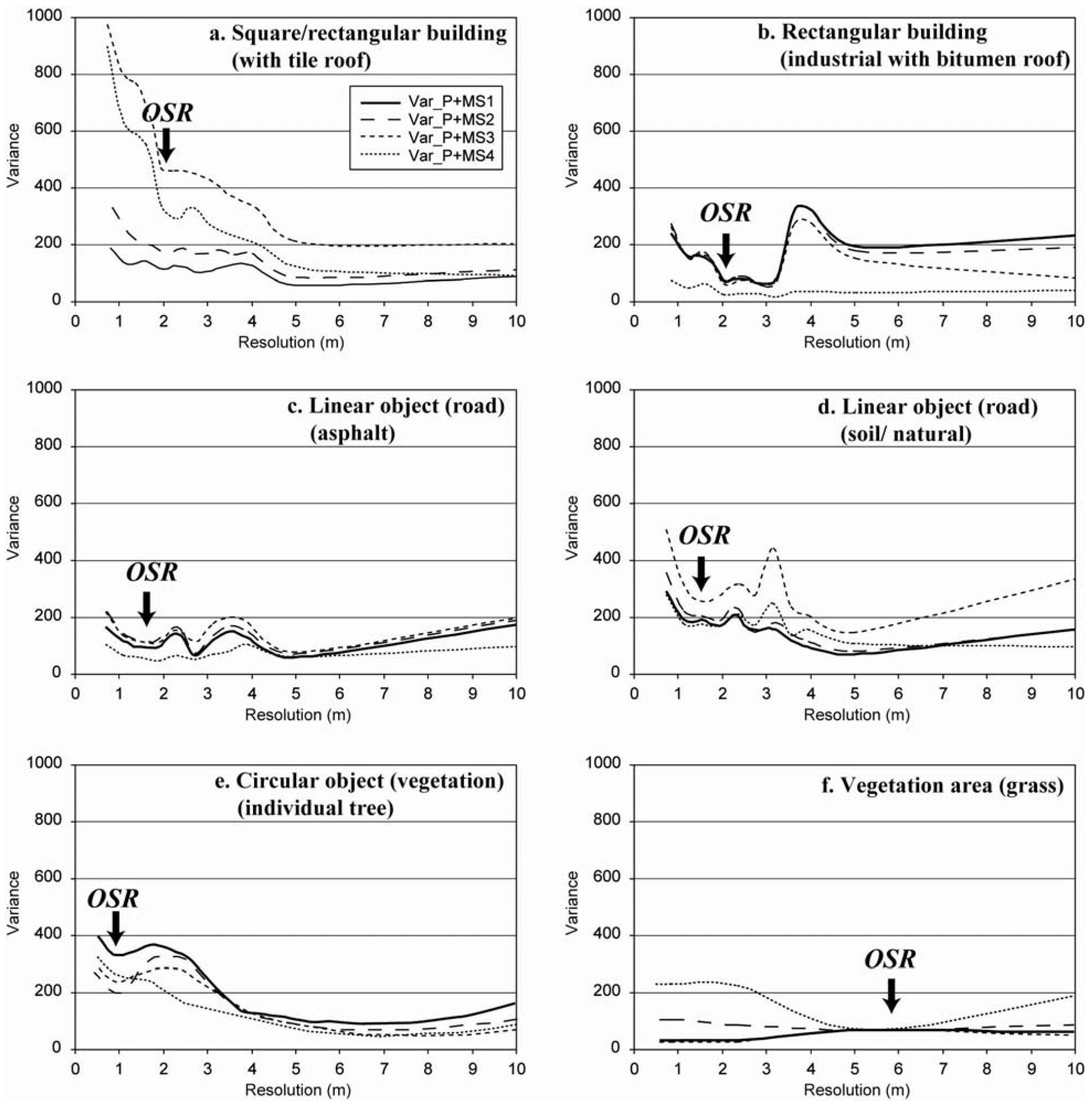
5. Results and Discussion

The results obtained at the two levels of observation indicate that each valley of the curves of variance in relation to spatial resolution can be interpreted in terms of a particular aggregation level (Figure 7 and Figure 8). Each curve shows the variation of local variance for each fused band from 0.7 m to 10.5 m at urban object level and from 10 m to 100 m for urban district level.

Figure 7. Local variance from the mean values and OSR for urban objects (Strasbourg, France).

Figure 7. Local variance from the mean values and OSR for urban objects (Strasbourg, France).

Figure 8. Local variance from the mean of the standard deviation values, OSR and fractal dimension for urban districts (Da Nang, Vietnam).

Figure 8. Local variance from the mean of the standard deviation values, OSR and fractal dimension for urban districts (Da Nang, Vietnam).

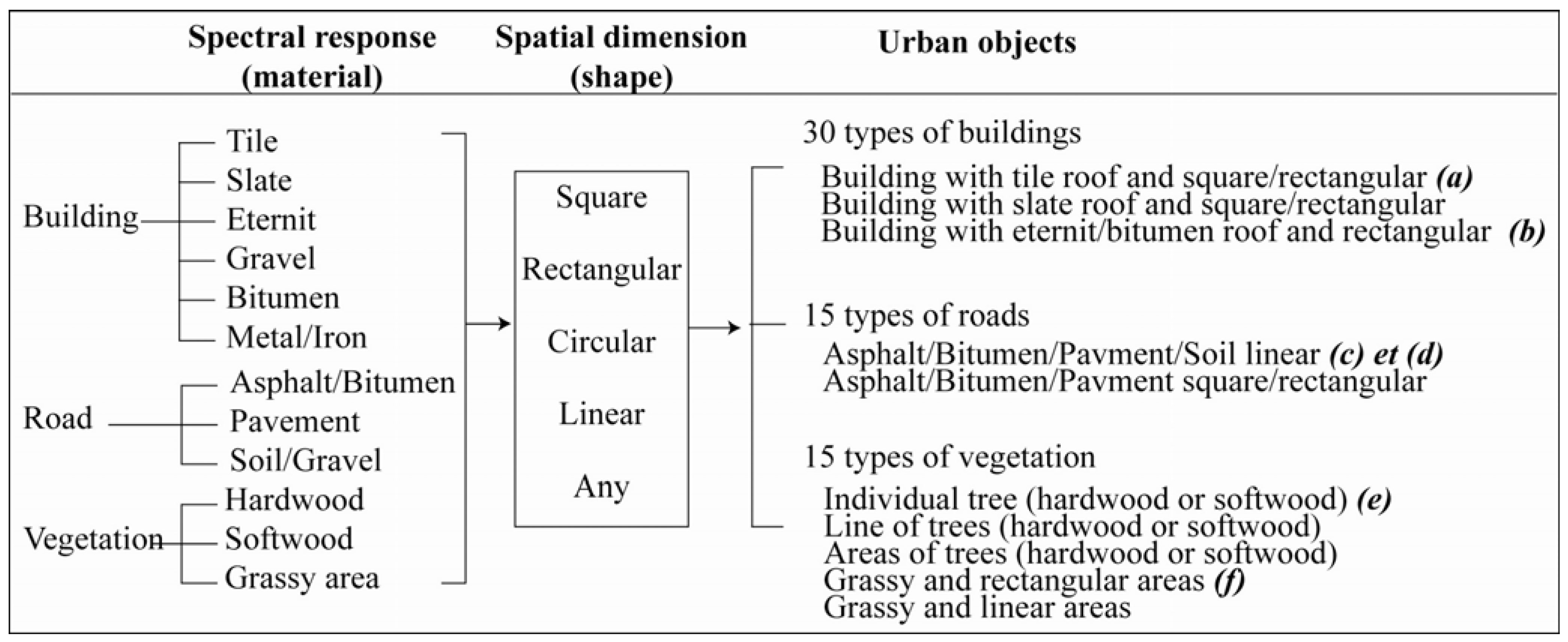
5.1. Results of Urban Objects (France)

Only curves of variance of some urban objects—most recurrent obtained from the pan-sharpened Quickbird image—are presented here in Figure 7. A first analysis of the whole curves of variance indicates different trends according to the type of urban objects but this tendency is the same whatever the spectral band.

For buildings with square and rectangular form (Figure 7(a,b)), the variance is firstly high at 0.7 m and decreases until the resolution from 2 to 3 m. Above this threshold, the variance increases until a resolution of 4 to 5 m, before reducing again. The first threshold corresponds to OSR where, for example, the roof of a building appears as the most homogeneous. Then, the more the spatial resolution is degraded, the more the mixels will appear in the border of objects sampling. This explains the increase of variance. Above a resolution of 5 m, the variance decreases because the object is integrated to its environment. The object is no longer identifiable because it belongs to a heterogeneous area due to the increased number of mixels. For elementary linear objects (road— Figure 7(c,d)), the same trend is observed with the OSR less than 2 m. For elementary objects such as individual tree, the OSR varies between 0.7 m and 1 m (Figure 7(e)). Finally, for large areas of any forms (urban forest, grassy area) that have homogeneous surfaces, the minimal variance is determined at progressively coarser resolution. The OSR becomes coarser, near 6 m (Figure 7(f)). When the size of objects decreases, the OSR decreases also.

5.2. Results at Urban Districts (Vietnam)

The aggregation process highlights the local variance of urban structures according to the spatial precision of the images used. We obtained different curves of variance according to the structure of city districts. We found that the NIR and MIR1 bands of pan-sharpened Spot and Landsat ETM+ are the most determinant (Figure 8). Their curves are very typical and allow defining the thresholds at which different city districts may be identified.

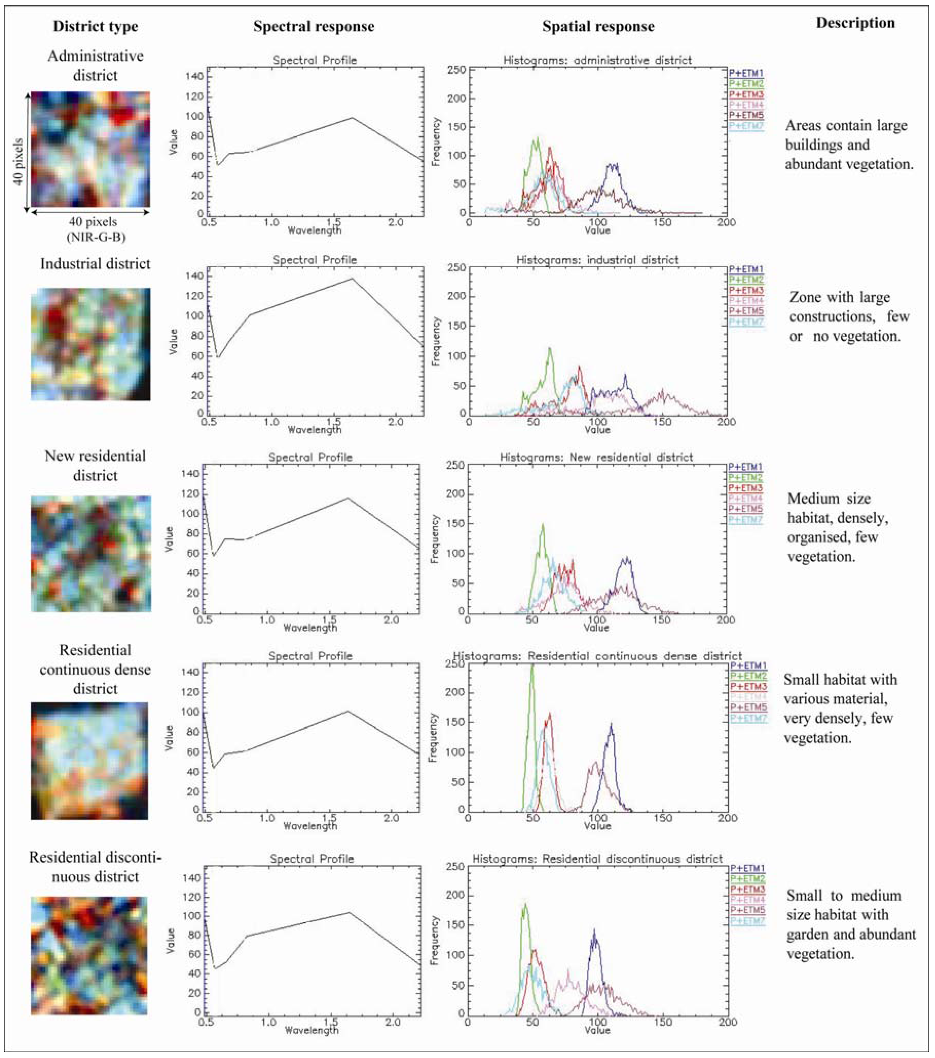
The administrative districts (administrative buildings, old colonial buildings) (Figure 8(a)) have great blocks and large-sized buildings. Their variances firstly present high at 10 m and decrease until 30–40 m. Above these thresholds, the variance increases again until a resolution of 60 m then finally decreases again. This range of thresholds corresponds to the OSR at which constitutive features of spatial organizations of city districts appear. The increase of variance of these two thresholds refers to mixels which increase the heterogeneity of constitutive features inside the samplings. Thereafter, the variance declines with decreasing resolution due to increased mixels.

We observed the same trend for other city districts. For example, in the case of industrial districts, OSR is situated always between 50 m and 60 m (Figure 8(b)) while the others such as new residential districts (Figure 8(c)) or residential discontinuous districts (Figure 8(e)) have an OSR range varying from 30 m to 40 m. The residential continuous dense districts consequently show an OSR of between 20 m and 30 m (Figure 8(d)). We also tried to identify the spontaneous districts but this was not possible due to reduced size of constitutive elements from available images. These require higher spatial resolution, at least 5 m, because of the reduced-size of houses.

6. Identification of Threshold of Heterogeneity/Homogeneity of Built-Up and Vegetation

The local variance allows us to identify a range of optimal pixel sizes at which urban objects/districts have the best representation for local detection. However how is the urban structure organized at this range of optimal pixel size? Urban space is known largely by its high complexity of land cover. Therefore, does the OSR present the threshold of heterogeneity/homogeneity at which urban structure is better distinguishable? In order to take into account these aspects, we use the fractal dimension issue of the box-counting method [43,44,45] to measure the spatial organization of two base elements of landscape: built-up and vegetation. We consider that at the threshold of homogeneity, spatial organization of built-up and vegetation is quite homogeneous; and their fractal dimensions at this threshold will get maximal values.

The built-up area is extracted from classification results of pan-sharpened image of Spot and Landsat ETM+ while the vegetation is computed from the Normalized Difference Vegetation Index (NDVI) which is related to the proportion of photosynthetically absorbed radiation, calculated from the red (R) and near infrared (NIR) channels of this pan-sharpened image by following formula:

$$NDVI=\frac{NIR-R}{NIR+R}$$

NDVI values vary between −1.0 and 1.0. Higher values are associated to higher levels of healthy vegetation cover.

Fractal dimension appears as a useful measure of spatial heterogeneity offering the advantage of variability across scale. It is calculated by formula:

$$\mathrm{D}=\frac{\mathrm{Log}({\mathrm{N}}_{\mathrm{ij}})}{\mathrm{Log}({\mathrm{r}}_{\mathrm{j}})}$$

with D: the fractal dimension from the box-counting method,

N_ij:

the number of built-up pixels or vegetation pixels of district sample i (1~3) at the pixel size j,

r_j:

the box size j corresponding to the number of pixels covering the length of the side of subset image at the pixel size j.

Fractal dimensions can take a range from 0 to 2. Low fractal dimension characterizes heterogeneous patterns while high fractal dimension corresponds to homogeneous structures. Fractal dimensions of built-up and vegetation are computed by the mean fractal values of three samples of each type of districts at each pixel size. Are the thresholds of spatial heterogeneity/homogeneity for built-up and vegetation coherent with the resulting fractal dimensions?

6.1. Spatial Distribution of Built-Up Within Urban Districts

According to the presence and to the compactness of built-up space, the fractal dimensions of built-up (D_built-up, red curve in Figure 8) of the administrative, industrial, new residential, and residential continuous dense districts have very high values, close to 2 (Figure 8(a–d)). This observation is particularly convergent to results obtained by [13] because of high compactness of built-up environment. The structure of these districts is not changed despite the aggregation level.

Fractal dimensions of built-up administrative, new residential and residential continuous dense districts are constant and equal to 2 through pixel size (Figure 8(a,c,d)). This explains that buildings for which the components of urban structure are densely distributed within urban landscape, consequently create invariant aggregates. When pixel size of image is degraded, these buildings maintain their forms and also their fractal dimensions.

The industrial districts characterized by large buildings size, storage places, etc. as well as their irregular distributions in the space, cannot preserve their initial form through degrading pixel size. Therefore, fractal dimensions decrease continuously when pixel size is increased from 10 to 100 m (Figure 8(b)).

The residential discontinuous districts characterized by low built-up presence and by open space between buildings, thus have low fractal dimensions. They lose initial form by increasing pixel size and so fractal dimensions diminish from 10 to 100 m with a lower peak between 70 and 80 m (Figure 8(e)).

Mostly, the threshold of homogeneity/heterogeneity for built-up area in all urban districts is not strictly identified because fractal dimensions get the maximal values close to 2 across aggregation level. We suppose that the dense built-up area of these samples illustrates a strong compactness. So the fractal dimension values are identical through pixel sizes.

6.2. Spatial Distribution of Vegetation within Urban Districts

Inversely to the built-up area occupying all urban districts, vegetation through NDVI presents little surfaces in administrative, industrial, new residential and residential continuous dense districts. The fractal dimensions of vegetation (D_NDVI, green curve in Figure 8) of these districts consequently are small and vary according to the increasing pixel size (Figure 8(a–c)) and particularly residential continuous dense districts (Figure 8(d)).

The only residential discontinuous districts characterized by vegetation abundance and continuous distribution of vegetation have high values of fractal dimension (Figure 8(e)). In fact, important vegetation distribution induces high fractal dimensions through degradation of spatial resolution. These values vary slightly according to the different spatial resolutions.

In general, these results of vegetation analysis indicate that the presence and the spatial distribution of the elementary objects in urban landscape are observed through the threshold of homogeneity. This homogeneity varies according to the type of urban district and to the spatial relation between built-up and vegetation. If the urban area is compact or highly homogenous, the increasing pixel size does not influence the homogeneity of the built-up and thus fractal dimensions remain invariant. On the other hand, by observing the fractal dimensions curves of vegetation, we find that the pick of fractal values appears at 50–60 m pixel size at all urban districts except residential discontinuous ones. This essentially presents the threshold of homogeneity at which vegetation located in these districts keeps its representative distribution in the space. Out of this threshold, vegetation presence becomes very heterogeneous.

7. Conclusions

This manuscript focuses on the optimal pixel size according to urban objects characteristics and urban structure for automatic detection from remotely sensed imagery. The results show that the range of OSR for urban objects or districts is related closely to the urban structure and spectral variability. The local variance seems to be a relevant parameter for the determination of OSR at which elementary objects and urban structures are detectable. When the pixel size and the size of object are close, the local variance gets the minimal value corresponding to the OSR at which the object is better discriminated.

Because urban area is especially known for its heterogeneity, its complexity of land cover and its diversity in form, size, structure and material and the choice of areal units of objects of interest is arbitrary and modifiable (MAUP [20]). So, we propose a range of OSR for urban objects and urban districts. Our results highlight three categories of spatial resolutions for identifying OSR: from 0.8 m to 3 m for isolated objects, from 6 m to 8 m for vegetation area and equal to or higher than 20 m for urban fabric. At the urban district level, according to spatial patterns, form, size and material of elements, we propose a range of OSR between 30 m and 40 m for detection of administrative districts, new residential districts and residential discontinuous districts. The detection of industrial districts requires a coarser OSR, from 50 m to 60 m. The residential continuous dense districts effectively need a finer OSR of between 20 m and 30 m for optimum identification.

Finding a way to identify urban spatial organization by fractal dimensions involves complexity of urban structure. Urban area is known for its high complexity but it differs from urban districts according to the original spatial distribution of built-up and vegetation elements. The fractal dimensions result from the box-counting method and are not convergent. The high compactness of built-up areas leads to maintaining extremely strong fractal dimensions across aggregation pixel level for all urban districts. Therefore, we cannot determine a threshold of homogeneity for built-up space by fractal dimensions. However, we found a threshold of homogeneity for vegetation areas between 50–60 m of pixel size at which fractal dimensions of vegetation are chosen. In addition, we established that the range of OSR does not exactly correspond to the threshold of homogeneity (except for industrial districts) which may be due to the high compactness of urban areas in the city of Da Nang.

Using urban remote sensing allows designing a procedure of knowledge extraction at several levels of observation: agglomeration, district and object. The local variance establishes a range of adequate pixel sizes at which urban districts are observable. This indicator is a function of the pixel size and the size of objects within districts. It does not enable understanding the structure and spatial distribution of these objects. In contrast, the fractal dimension characterized by the principle of homogeneity/heterogeneity of the spatial organization highlights the urban structure of the city of Da Nang. Our approaches show the potential of using these complementary methods for urban form detection and urban structure identification whatever the study areas. The results obtained confirm the existence of scale effect and aggregation effect [20] when we work on different scales and sizes of units.