Feasibility of Invasive Grass Detection in a Desertscrub Community Using Hyperspectral Field Measurements and Landsat TM Imagery

Abstract

Invasive species’ phenologies often contrast with those of native species, representing opportunities for detection of invasive species with multi-temporal remote sensing. Detection is especially critical for ecosystem-transforming species that facilitate changes in disturbance regimes. The African C₄ grass, Pennisetum ciliare, is transforming ecosystems on three continents and a number of neotropical islands by introducing a grass-fire cycle. However, previous attempts at discriminating P. ciliare in North America using multi-spectral imagery have been unsuccessful. In this paper, we integrate field measurements of hyperspectral plant species signatures and canopy cover with multi-temporal spectral analysis to identify opportunities for detection using moderate-resolution multi-spectral imagery. By applying these results to Landsat TM imagery, we show that multi-spectral discrimination of P. ciliare in heterogeneous mixed desert scrub is feasible, but only at high abundance levels that may have limited value to land managers seeking to control invasion. Much higher discriminability is possible with hyperspectral shortwave infrared imagery because of differences in non-photosynthetic vegetation in uninvaded and invaded landscapes during dormant seasons but these spectra are unavailable in multispectral sensors. Therefore, we recommend hyperspectral imagery for distinguishing invasive grass-dominated landscapes from uninvaded desert scrub.

1. Introduction

Biological invasions are drastically altering ecosystems worldwide. Particularly problematic are those that alter disturbance regimes [1,2,3,4,5]. In subtropical regions of North America, South America, Australia, and neotropical islands, African C₄ grasses are introducing a grass-fire cycle that results in rapid transformation of invaded ecosystems [1,4]. In North America’s Sonoran Desert, Pennisetum ciliare, Pennisetum setaceum, Eragrostis lehmanniana, Eragrostis cilianensis, Melinis repens, and Enneapogon cenchroides are expanding in desert scrub habitats poorly adapted to fire [5,6]. P.ciliare (buffelgrass) has already reached epidemic proportions, prompting the formation of a Buffelgrass Coordination Center and a noxious weed listing by the state of Arizona [5,7]. Primary concerns relate to the consequences of fire on the Arizona Upland vegetation zone of the Sonoran Desert, a vegetation known for its scenic beauty and high biodiversity [5,7]. The regional importance of this ecosystem is embodied by Saguaro National Park, a federally-managed wilderness area dedicated to preserving the giant saguaro columnar cactus (Carnegeia gigantea) and other native biota. In addition, much of the vibrant tourism industry of southern Arizona is built around the picturesque columnar cacti, stem and leaf succulents, trees with photosynthetic bark, and the wildlife that depends on this diverse vegetation community. P. ciliare threatens to unravel this ecosystem, not only leaving the tourism industry to adapt to a frequently-burning grassland, but Sonoran Desert residents with a potent new hazard to life and property.

Of utmost importance to all ecosystem managers faced with P. ciliare invasion is the development of repeatable methods for regional-scale mapping and monitoring [7]. However, previous attempts to utilize remote sensing data to identify and classify P. ciliare have been unsuccessful without manual interpretation of high spatial-resolution photographs [8,9,10]. Given the legacy and availability of Landsat MSS/TM/ETM+ imagery and the similarity in band characteristics of other modern multispectral sensors (e.g., SPOT High Resolution Visible sensor, Advanced Land Imager, Indian Remote Sensing Satellite 1D), it is important to assess the feasibility of using multispectral sensors for detecting P. ciliare.

1.1. Background

The Arizona Upland vegetation zone occupies the northernmost reaches of the Sonoran Desert, where cold temperatures limit the distribution of the mixed cactus forest characteristic of this desert [11]. Perennial vegetative cover of medium-sized trees, shrubs, sub-shrubs, upright cacti, prostrate stem succulents, perennial vines, and forbs is typically <30% [11]. Mineral soils are poorly developed, rocky, and dominate the land cover as seen from above [12]. Seasonal flushes of vegetative growth may temporarily increase cover as annuals, drought-desiccant mosses, and drought-deciduous plants respond to precipitation in a bimodal growing season [13].

P. ciliare grows under trees and shrubs and fills in the interstitial spaces between them, creating a well-connected grassland [5,8,14,15] (Figure 1). Over time, native species richness and diversity decline, leaving a monoculture of fine flammable fuels [15]. It is important to detect and manage these infestations before this transformation occurs because of the disproportionate role that small remote patches of P. ciliare play in furthering the spread of this species and the decreasing likelihood of management success with time since invasion [3,16]. Given this management need, we seek strategies that will result in the detection of infestations at low levels before transformation occurs. Towards this end, we recognize that there are several key differences between native vegetation and P. ciliare-dominated areas that may be helpful in discriminating the two via remote sensing methods:

(1)

From the standpoint of cover, P. ciliare replaces soil. Sub-canopy P. ciliare is less likely to have a profound effect on reflectance of a mixed pixel.

(2)

Native grasses do not form dense stands in the upland habitats in which P. ciliare is invading.

(3)

P. ciliare is visible from a distance with the human eye at different times of the year.

Other attempts have been made to discriminate P. ciliare from native vegetation. Franklin and others utilized Landsat TM in combination with aerial overflights and ground-based methods to estimate the extent of P. ciliare landscape conversion in the state of Sonora, Mexico, where it is planted in pastures [8]. Although they were able to identify the extents of pastures, they were not able to identify P. ciliare itself without ground validation. Similarly, Brenner used image segmentation to identify pastures but was unable to determine species composition within a pasture without a corresponding ground observation [9]. In both cases, P. ciliare-dominated pixels were too similar to uninvaded areas. This is largely due to the phenological synchrony that most species have in the Sonoran Desert in response to seasonal precipitation due to the strong water limitation at all other times of the year.

It has been previously noted that Landsat TM is unable to distinguish between soil and non-photosyntetic vegetation (NPV) due to the inability to resolve cellulose absorption at 2,100 nm with the wide-bandwidth of the short-wave infrared bands [17]. However, distinguishing between photosynthetic vegetation (PV) and soil with Landsat TM is well-established [18,19,20]. If we assume that soil remains soil throughout the year and that P. ciliare resembles NPV (and, hence, soil) in the arid fore-summer, but looks like PV following the summer monsoons, then a classifier that captures this Soil-to-PV transition may be viable.

Figure 1. Photos of four P. ciliare-infested hot spots identified in the Santa Catalina Mountains. P. ciliare stands out in these images by its golden hue and smooth texture, which contrasts from the beige tones and speckle associated with uninvaded areas. The golden hue is characteristic of post-monsoon curing and although the golden hue fades, standing senesced vegetation remains a fuel concern throughout the year. The homogeneous texture is characteristic of connected grass cover, whereas the heterogeneous textures of uninvaded habitat represents a mixture of exposed soil, rocks, shrubs, cacti, and trees.

Figure 1. Photos of four P. ciliare-infested hot spots identified in the Santa Catalina Mountains. P. ciliare stands out in these images by its golden hue and smooth texture, which contrasts from the beige tones and speckle associated with uninvaded areas. The golden hue is characteristic of post-monsoon curing and although the golden hue fades, standing senesced vegetation remains a fuel concern throughout the year. The homogeneous texture is characteristic of connected grass cover, whereas the heterogeneous textures of uninvaded habitat represents a mixture of exposed soil, rocks, shrubs, cacti, and trees.

1.2. Objectives

The main objective of this paper is to assess the feasibility of using multi-spectral imagery to identify Pennisetum ciliare in desert scrub habitats of the Arizona Upland. More specifically, we define the following objectives to guide our research and highlight potential causes for confusion and more accurate results:

(1)

Identify spectral characteristics that distinguish P. ciliare from uninvaded Arizona Upland cover types throughout the year

(2)

Determine best time of year to discriminate between P. ciliare and uninvaded Arizona Upland vegetation

(3)

Assess the potential of multi-date analysis to improve upon single-date analysis to discriminate between P. ciliare and uninvaded Arizona Upland vegetation

2. Data and Methods

This study is based on three components: (1) spectral analysis of uninvaded and invaded landscapes, (2) spectral classification of single- and multi-date simulated Landsat TM scenes, and (3) classification of single-and multi-date TM scenes. A flowchart describing the methodologies for simulated and real Landsat TM scenes are given in Figure 2.

Figure 2. Flow diagram indicates the source of simulated and real Landsat TM scenes and classification models.

Figure 2. Flow diagram indicates the source of simulated and real Landsat TM scenes and classification models.

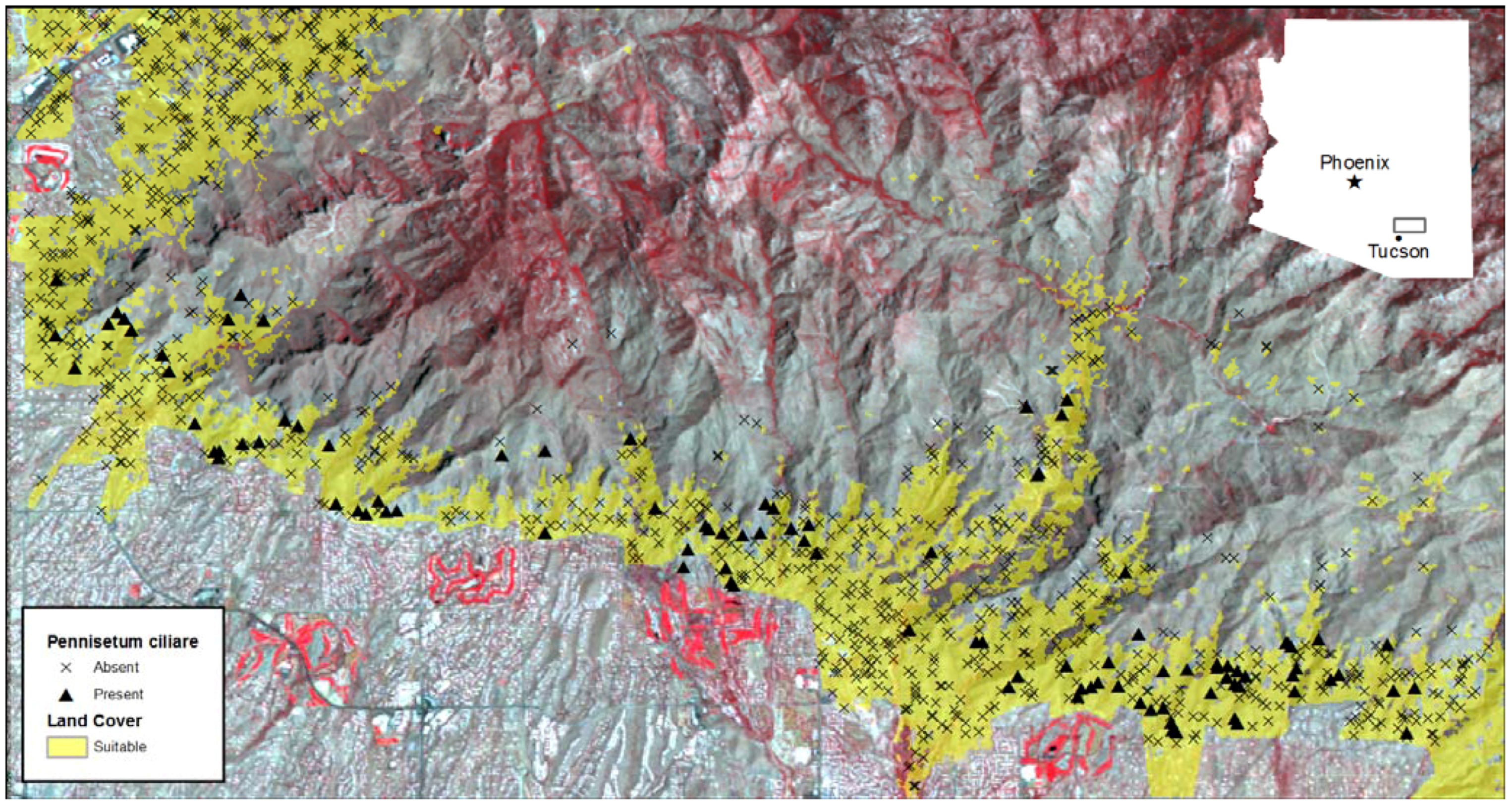
2.1. Study Area

This study was conducted in the Santa Catalina Mountains in Southern Arizona, USA, in habitat typical of the Arizona Upland, a subdivision of the Sonoran Desert [11]) (Figure 3). The Sonoran Desert is a hot desert with mean annual temperatures of 28.6 °C and four months with mean temperatures over 35 °C [21]. Precipitation (320 mm annually) is bimodally distributed, with slightly more precipitation falling during the summer [21]. The sparse canopy cover is dominated by the small tree Parkinsonia microphylla, the short-lived shrub (Encelia farinosa), and the saguaro cactus (Carnegiea gigantea) [11]. The landscape is remarkably diverse in species and lifeforms, including trees, shrubs, cacti, grasses, and forbs [11]. Vegetation responds rapidly to the onset of the North American Monsoon, after which a flush of annual and perennial growth briefly greens up the desert. Analysis was confined to four vegetation classes as defined by the Southwest Regional Gap Vegetation Analysis Project: Chihuahuan Succulent Desert Scrub (#55), Chihuahuan Creosotebush, Mixed Desert and Thorn Scrub (#56), Sonoran Paloverde-Mixed Cacti Desert Scrub (#57), and Sonoran Mid-Elevation Desert Scrub (#105) [22]. These classes represent habitat most threatened by P. ciliare [6].

Figure 3. Map of study area showing validation points overlaid on Landsat TM Image from 26 May 2007 (path 36, row 38). The yellow overlay shows Southwest Regional GAP Analysis cover classes in which P. ciliare is common.

Figure 3. Map of study area showing validation points overlaid on Landsat TM Image from 26 May 2007 (path 36, row 38). The yellow overlay shows Southwest Regional GAP Analysis cover classes in which P. ciliare is common.

2.2. Field Data Collection—Cover Measurements

In a separate study, projected perennial vascular plant canopy cover was measured in winter, 2008–2009, in 53 plots on south-facing piedmonts in mixed palo verde-cactus vegetation in the Santa Catalina Mountains [15]. Fifty-three plots measuring 11 m on a side were oriented along 10 transects covering a gradient of P. ciliare cover. Transects varied from four to nine plots in length. Elevation ranged from 883 to 1,097 m across the plots. 53 species were identified and measured in the plots, as well as rock, mineral soil, and NPV. Cover was estimated for each unique species and substrate using a point intercept at every 1m on a regular grid in the plot (100 points). Mean cover for species and cover types ranged from 0 to 28% with four cover types: Bare soil (28%), rock (16%), Encelia farinosa (16%), and Parkinsonia microphylla (14%) consistently comprising the four most abundant types in 15 uninvaded plots (n = 15 plots with <5% P. cliare). Cover of all types decreased in invaded plots with the most abundant cover types being bare soil (14%), rock (13%), NPV (6%), and P. microphylla (3%) (n = 21 plots with >50% P. ciliare). These 56 classes were the basis of a spectral analysis of P. ciliare separability from native cover types. For the present study, we consider the percent cover of each land cover type fixed between 16 March and 26 October 2007.

2.3. Field Data Collection—Spectral Data Acquisition

We measured hyperspectral reflectance of dominant plants and cover types at Tumamoc Hill on six dates during 2007. Tumamoc Hill (elev. 847 m) is characterized by vegetation typical of the Arizona Upland and also contains vigorous populations of P. ciliare [23]. Its accessibility and proximity to Tucson, AZ, made it ideally suited for field measurements of Arizona Upland vegetation. Spectra were collected using an ASD spectrometer (Analytic Spectral Devices, Inc) during cloud-free days between 10 am and 12 pm local time on 16 March, 16 April, 25 May, 16 August, 22 September, and 26 October of 2007.

The ASD was used to collect hyperspectral signatures from 350 nm to 2,500 nm in 2,151 spectral bands at nadir view angles and a 5° field-of-view. Each spectrum synthesized from the collection is a mean of five measurements taken of each target. During data collection, the instrument and data were regularly initialized and referenced to a Spectralon® calibration panel to compute surface reflectance values. Tumamoc Hill, where ASD measurements were taken place, is about 10km to the southeast of this map extent.

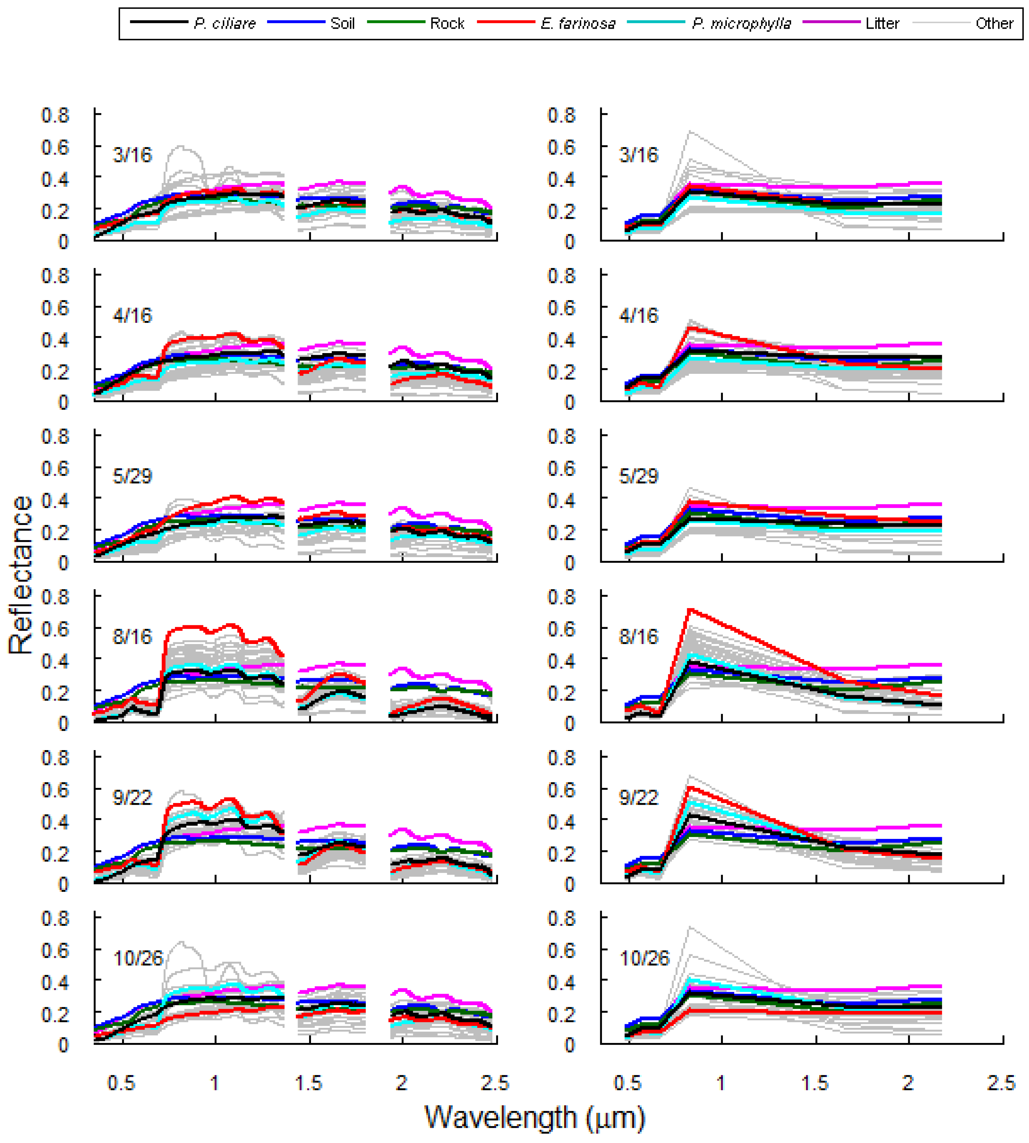
2.3. Spectral Separability of Pennisetum ciliare from Native Cover Types

Reflectance differences between P. ciliare and other cover types arise from differences in spectral reflectance (e.g., the presence or absence and position of absorption features in the spectra) and the magnitude (e.g., absolute reflectance). Correlation of spectral curves quantifies the similarities between two spectra with regards to shape while spectral differencing quantifies overall changes in brightness across the spectra. Atmospheric noise is significantly reduced by using the ASD at the surface; hence atmospheric water absorption windows (1,360–1,430 nm and 1,800–1,950 nm) were excluded from the analysis.

We calculated correlation of P. ciliare reflectance with all included species and cover types on each collection date to provide a measure of similar and contrasting cover types as they vary over time. While the landscape we are interested in is highly mixed, combinations of several cover types typically comprise greater than 50% of uninvaded cover: rock, soil, Encelia farinosa, Parkinsonia microphylla, and Prosopis glandulosa. We investigated the discriminability of P. ciliare from these dominant cover types in more detail, identifying the wavelengths that generate maximum differentiability for each season. Spectra were convolved to Landsat TM bandpass filters and correlations of convolved reflectance values were compared. To assess magnitude differences, we calculated the difference between the curves representing the reflectance of each cover type vs. P. ciliare.

2.4. Spectral Separability of Mixed Landscapes

We utilized plot-level cover measurements from Olsson et al.’s plant diversity study and predicted hyperspectral reflectance for all 53 plots for the six ASD reflectance data collection dates [15]. We divided plots into low (<5% P. ciliare cover), medium (5–50%), and high (≥50%) P. ciliare classes and performed a student’s t-test to test for differences between reflectance of high vs. medium and high vs. low at each wavelength. We did not correct for multiple comparisons.

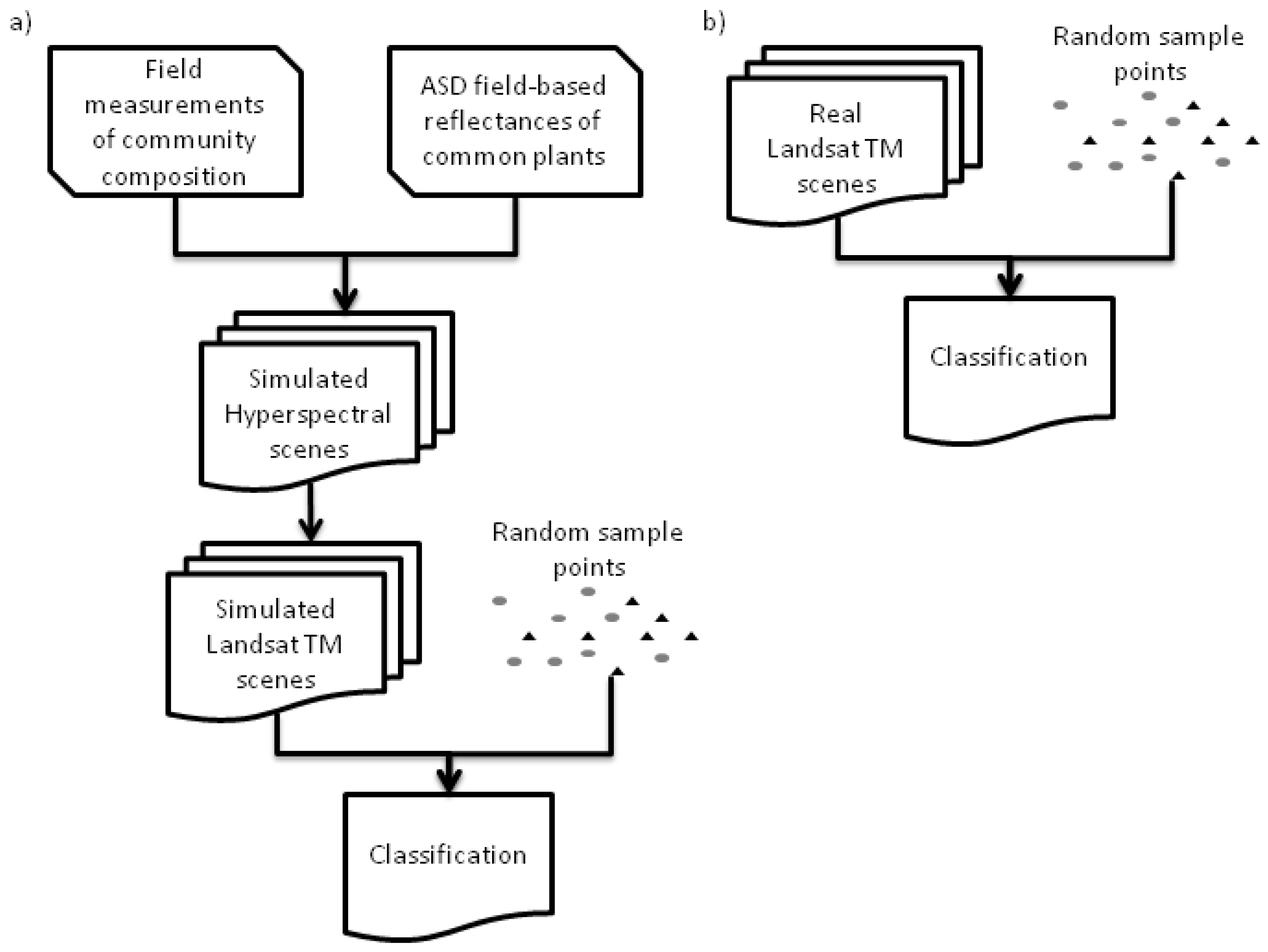
2.5. Simulated Landsat TM Scenes

Using plant abundances in uninvaded and invaded plots in a study by Olsson et al., we generated a 450 × 450 pixel landscape in which each pixel was a mixture of 56 cover types with abundance probabilities defined by the reference study [15]. Approximately 90% of cells were generated with no P. ciliare cover. Composition of the remaining cells was determined by fixing P. ciliare cover at a random value selected from a uniform distribution of values ranging from 5 to 90%. Simulated TM scenes were generated for each date that field spectra were available by assuming a linear mixture model and computing the weighted average of cover type abundances and reflectance values for each pixel. That is, Landsat TM reflectances were generated for each pixel using the formula:

$$\rho \left(x\right)={{\displaystyle \sum }}_{t=1}^{n}c\left(e,x,t\right)\rho \left(e,t\right)$$

(1)

where ρ(x) is the TM-convolved reflectance vector for the pixel at location x, n is the number of distinct components in the pixel, c(e,x,t) is the fractional abundance of cover type e, in pixel x, at time t, and ρ(e,t) is the Landsat TM-convolved reflectance vector for cover type e at time t. Although we chose Landsat TM, reflectances could have been convolved to any sensor bandpass. Simulated pixels were randomly grouped into equal-sized sets for training and validation.

2.6. Landsat TM Scenes

We acquired cloud-free Level 1T (systematic radiometric and geometric correction) Landsat TM imagery for WRS2 path 36, row 38 from the USGS GLOVIS portal (http://glovis.usgs.gov) from one date in 2008 (21 January), four dates in 2007 (8 April, 26 May, 14 August, 30 August) and one in 2006 (30 October). We were forced to utilize the scene from 2006 to assess possible autumn spectral differences due to all autumn TM scenes from 2007 being contaminated by cloud cover. Scenes were converted to atmospherically corrected surface reflectance using the cosine approximation model (COST) [24]. Corrected scenes were clipped to the study area.

2.7. Landsat TM Training and Validation Sites

USGS 1m Digital Orthophoto Quarter Quads acquired in 2007 were used to identify training points for dominant classes found in the TM scenes, including forest, riparian, desert scrub, rock outcrop, urban, bare soil, golf courses, and dense P. ciliare patches. An independent validation dataset was developed by classifying over 1,000 randomly generated points into three classes of P. ciliare based on a 30 × 30 m area surrounding each point using heads up digitizing via high-resolution imagery [10]. The three classes of P. ciliare infestation were defines as Low (<5%), Moderate (5–50%), and Heavy (≥50%). Random points were generated using Hawth’s Tools [25]. In a report to the Desert Southwest Cooperative Ecosystem Studies Unit, Olsson et al. confirmed heads up digitizing via high-resolution imagery as a viable method for mapping P. ciliare in some mixed scrub environments [10]. Note that the lowest category of P. ciliare infestation was primarily composed of P. ciliare-free areas, but at the resolution of the aerial photography it was not possible to confirm complete P. ciliare absence.

2.8. Scene Classification—Classification Data Models

We classified a variety of derived data models for all dates separately and combined using CART and logistic regression using Matlab 2009A. The following data models were used as input into the predictive models:

• Pure reflective (Refl)
• Spectrally unmixed PV, soil, and NPV (SMA_All)
• Spectrally unmixed PV (SMA_PV)
• Normalized Vegetation Difference Index (NDVI)
• Soil-adjusted Vegetation Index (SAVI)
• Enhanced Vegetation Index (EVI)

The six Landsat TM reflectance bands comprise the pure reflective data model (Refl). Spectral mixture analysis was performed on the reflectance data to generate a 3-band data model comprising fractional abundances of photosynthetic vegetation (PV), non-photosynthetic vegetation (NPV) and soil. Simulated TM endmembers were chosen from our previously acquired field spectra. The PV endmember was the actively growing P. ciliare plant from August while NPV was chosen as the senesced P. ciliare from May and the soil endmember was also selected from the May collection. Real TM endmembers for soil, PV, and NPV were chosen and extracted from the Landsat TM scenes using heads-up digitizing of DOQQs. The soil spectrum was from an exposed soil in a dry sandy river bottom in April, the vegetation spectrum was extracted from a golf course fairway during October, and the NPV spectrum was based on an area of dense senescent P. ciliare during April. Field based spectral endmembers were not utilized in the Landsat TM classifications because the magnitudes of the scene spectra did not match the field-derived spectra. (Multiple atmospheric correction algorithms were applied (e.g., COST [24], 6S [26]) but none provided an adequate absolute match). Data for all scenes were decomposed into fractional abundances using unconstrained spectral mixture analysis [27]. Specifically, abundances were calculated using a Moore-Penrose pseudo-inverse calculation in Matlab R2009A [28]. If the abundance of an endmember was negative, it was excluded, set to 0% and remaining endmember abundances were based on a 2-endmember mixture.

The remaining four data models are one-band data models based on either fractional vegetative cover (SMA_PV) or vegetation indices (NDVI, EVI, and SAVI). NDVI is the most prevalent vegetation index and is based on the contrast between the NIR reflectance, where plants are highly reflectance, and red reflectance, where actively photosynthesizing vegetation is strongly absorptive [18].

NDVI = (NIR − Red)/(NIR + Red)

(2)

In arid ecosystems such as the Sonoran Desert, soil is such a dominant cover fraction that soil brightness contamination is likely [12]. This was the impetus for the Soil-Adjusted Vegetation Index (SAVI), which uses a soil brightness-dependent correction factor, L, which Huete et al. suggested setting to 0.5 [12]:

SAVI = (1 + L)(NIR − Red)/(NIR + Red + L)

(3)

Additional criticisms of the NDVI model concern its sensitivity to atmospheric conditions. The Enhanced Vegetation Index (EVI) was developed to diminish the effect of atmosphere and improve sensitivity to high biomass [29].

EVI = G × (NIR − Red)/(NIR + C1 × Red − C2 × Blue + L)

(4)

where L is the soil background adjustment term and C1 and C2 are atmospheric adjustment coefficients. In this study, we use the MODIS coefficients: L = 1, C1 = 6, C2 = 7.5, and G = 2.5.

The four vegetation models are composed of single bands. In multi-date classifications, indices were selected from each date such that the total number of bands equals the number of dates. The six data models were utilized as explanatory variables in predictive models for single-date classifications for each date and as well as a combined model utilizing data models in a six-date stack.

2.9. Classification and Regression Trees (CART)

Classification and regression tree (CART) is a non-parametric technique for classifying input data (x) into continuous or discrete classes (y). A CART model is a binary search tree that maximizes the total drop in deviance by dividing the tree into successively more homogeneous subsets [30]. CART model accuracy was assessed by comparing the true positive rate, false positive rate, and overall classification accuracy using validation data.

2.10. Logistic Regression

Logistic regression is a generalized linear model for predicting the likelihood of a binary outcome (y) given a set of predictor variables (x) [31]. The goal of logistic regression is to find parameters, b for x that maximize the goodness of fit of the link function:

x × b = ln(µ/(1 − µ))

(5)

where µ is the mean of the binomial distribution given by y. The logistic regression model can be used to calculate likelihood values based on alternative values of predictor variables. An advantage of logistic regression is that likelihood values are continuous and binary classification can be based on thresholding at any level between 0 and 1. Consequently, overall model discrimination can be assessed by calculating the area under the Receiver Operator Characteristic, or ROC, curve [32]. Logistic regression models in this study were evaluated by the area under the ROC curve, which is denoted by the acronym AUC.

2.11. Landsat TM Scene Visualization

Based on perceived differences in seasonal PV fluctuations of P. ciliare vs. desertscrub, we created a series of false color composite using various combinations of scene dates, model outputs, and RGB channels. We selected three models in which known P. ciliare patches were discernable by their pattern and determined a suitable combination for display based on permutations of models with color channels in RGB and CMYK color space. Because many models were dominated by very high or very low values, we employed various transforms of data, including inversion.

3. Analysis of Results

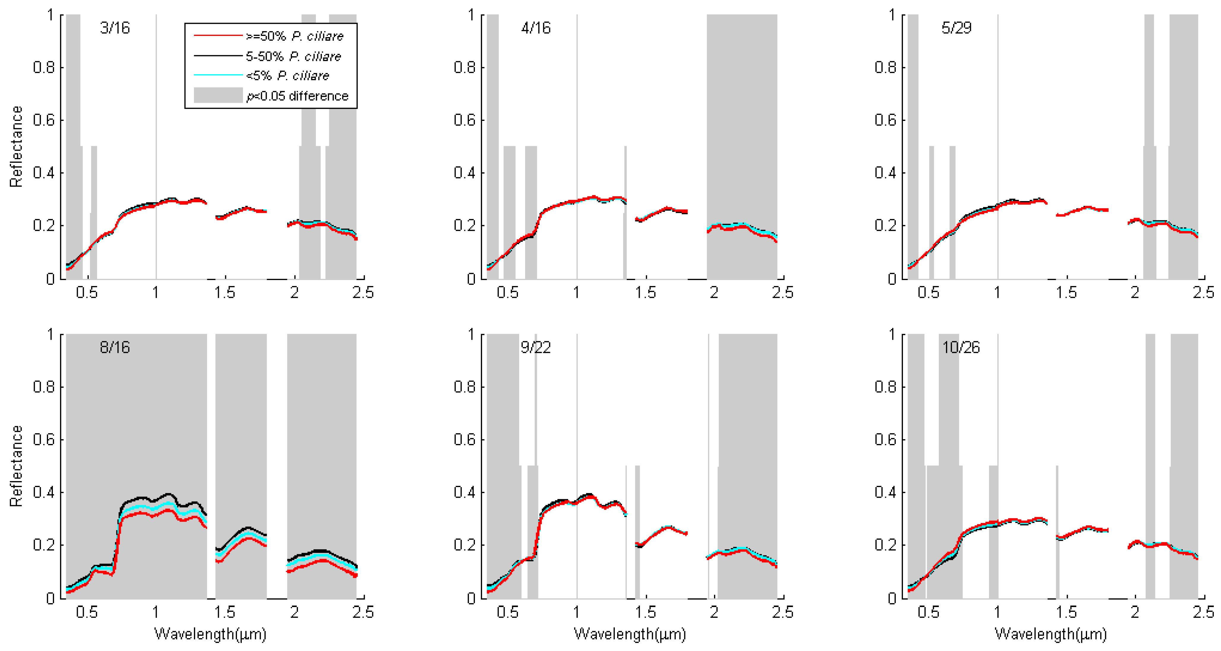
3.1. Spectral Separability of Pennisetum ciliare Over Time

Hyperspectral and TM-convolved reflectance data for all six field dates are shown in Figure 4. Spectra of all vegetative classes changed over the course of the year, with all species showing a slight-green-up signal (i.e., red absorption at 680 nm) in the two spring dates (March and April), followed by a decline in the arid fore-summer (May). Inspection of the reflectance curves of the dominant cover types on all six field spectra collection dates reveals P. ciliare resembles soil, NPV, and P. microphylla in different spectral regions at different times of the year. P. ciliare exhibits a red absorption minimum (680 nm) and red edge (680–720 nm) in March, April, and May that distinguishes it from soil, rock, and NPV, although this separation is lowest in May when Sonoran Desert plants are less photosynthetically inactive. Another characteristic pattern is the strong resemblance of P. ciliare in the 1,400–1,800 nm (SWIR1) and 1,980–2,400 nm (SWIR2) regions to the reference NPV spectrum in all dates except August and September, although even in September the NPV absorption feature at 2,000 nm is evident in P. ciliare. While P. ciliare resembles NPV in these SWIR regions during periods that are dry or drying, the shape of its VNIR reflectance curve more closely resembles soil or rock during the hottest, driest part of the year (25 May). Unfortunately, the complexities of reflectance shape changes in SWIR1 and SWIR2 over the year are lost in the convolution to TM. The absorption feature is lost in the convolution and NPV is not distinct from soil, rock, or vegetation.

Correlations of hyperspectral and TM-convolved P. ciliare reflectance data with other dominant cover types are shown Figure 5. Correlations with soil, rock, and NPV were lower than correlations with other vegetation on all dates—most notably in August, September and, to a lesser extent, in April. Maximum correlation occurred on 16 August for all vegetation and on 29 May for all other cover types in both hyperspectral and TM-convolved spectral space.

Minimum correlation for P. microphylla and P. glandulosa occurred on 26 October in hyperspectral space, but only occurred on the same date for P. microphylla in TM space. Correlation was lowest for P. glandulosa in the March 16 TM-convolved spectra. E. farinosa correlation also differed between the hyperspectral and TM-convolved spectra with minima occurring on 22 September and 26 October, respectively.

The integrated reflectance differences, also shown in Figure 6, portray similar discriminability of P. ciliare from soil, rock, and NPV, with maximum differences occurring on 16 August for all three cover types and minimum differences occurring on 29 May for both rock and NPV while soil had minimum integrated difference on 16 March. Integrated reflectance differences differ from correlation, however.

For example, E. farinosa had the greatest difference on 16 August for both hyperspectral and TM-convolved reflectance, the same date its correlation was maximized. Its minimum occurred on 16 March for both types of spectra. P. glandulosa differences were maximized on 16 August (hyperspectral) and 16 March (TM-convolved) and minimized on 22 September (both spectral types). Only P. microphylla had differences that complemented correlation, having minimum and maximum differences for both spectral types on 16 August and 16 March, respectively (26 October differences were similar to March differences).

Figure 4. Reflectance of abundant cover types found in measured plots on six different dates in 2007 as measured by ASD (left column) and convolved to Landsat TM (right column). P. ciliare is denoted by a thick black line while five dominant native cover types are denoted by thick colored lines. Less abundant cover types are light grey.

Figure 4. Reflectance of abundant cover types found in measured plots on six different dates in 2007 as measured by ASD (left column) and convolved to Landsat TM (right column). P. ciliare is denoted by a thick black line while five dominant native cover types are denoted by thick colored lines. Less abundant cover types are light grey.

Figure 5. Correlation of reflectances (top row) and mean reflectance differences (bottom row) between P. ciliare and native cover types for full spectra (left column) and TM-convolved spectra (right column) for six dates in 2007. Five most abundant cover types are denoted by thick colored lines, whereas less abundant cover types are denoted by light grey.

Figure 5. Correlation of reflectances (top row) and mean reflectance differences (bottom row) between P. ciliare and native cover types for full spectra (left column) and TM-convolved spectra (right column) for six dates in 2007. Five most abundant cover types are denoted by thick colored lines, whereas less abundant cover types are denoted by light grey.

Figure 6. Reflectance differences of six abundant cover types by time (y-axis) and wavelength (x-axis). Positive values (blue) indicate the target is more reflective than P. ciliare for the given wavelength and acquisition date while negative values (green) indicate that P. ciliare is brighter.

Figure 6. Reflectance differences of six abundant cover types by time (y-axis) and wavelength (x-axis). Positive values (blue) indicate the target is more reflective than P. ciliare for the given wavelength and acquisition date while negative values (green) indicate that P. ciliare is brighter.

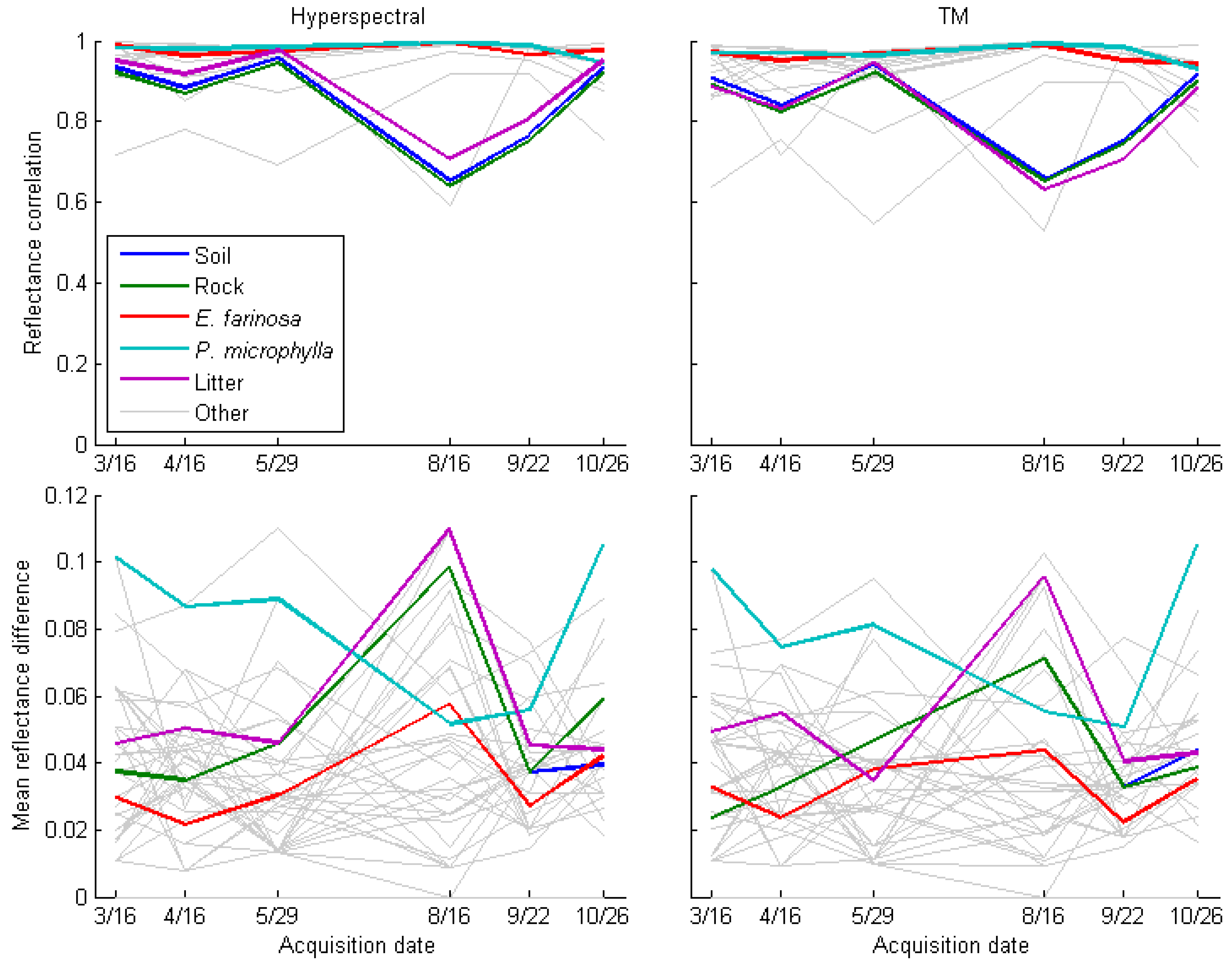
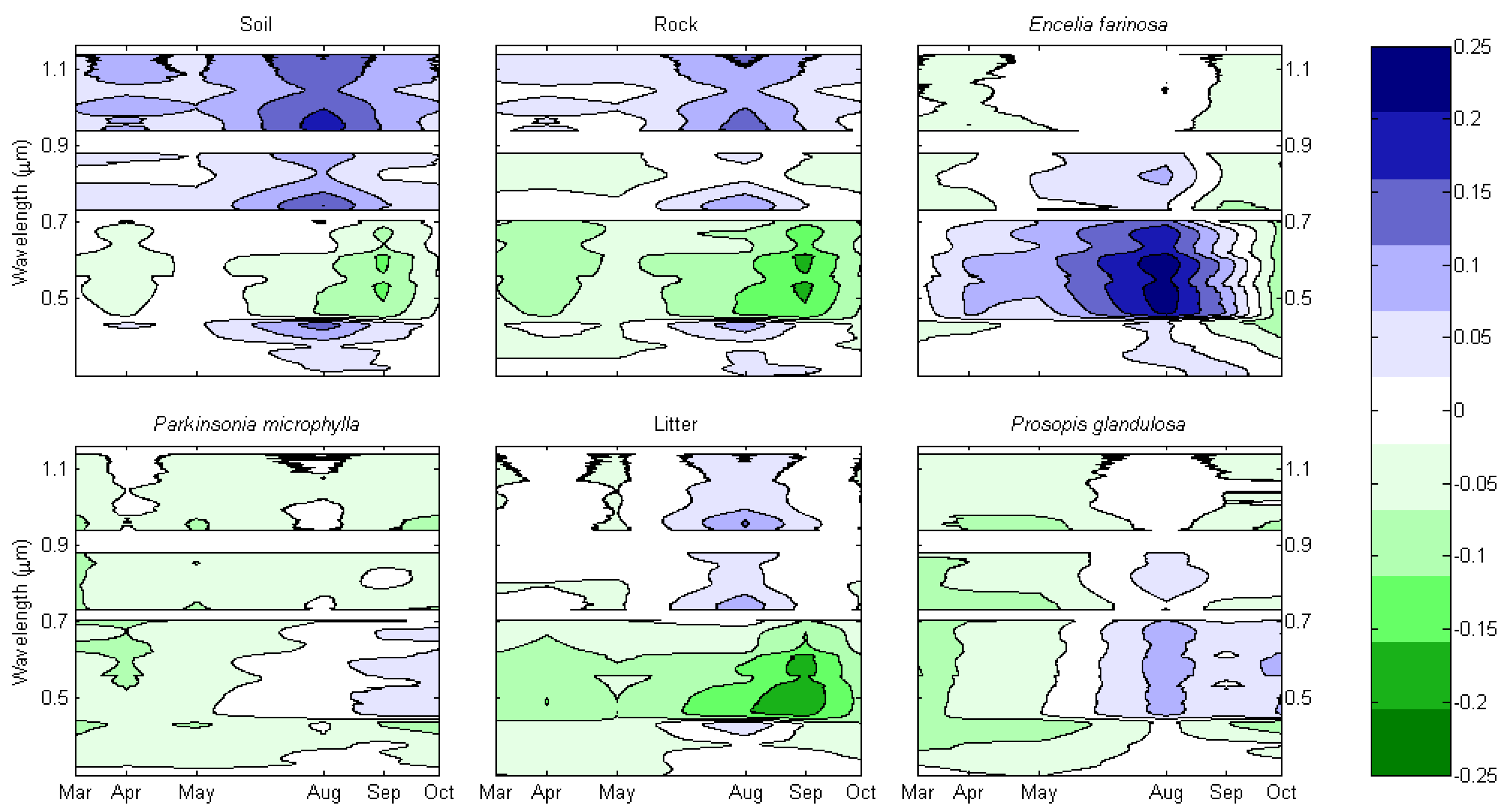
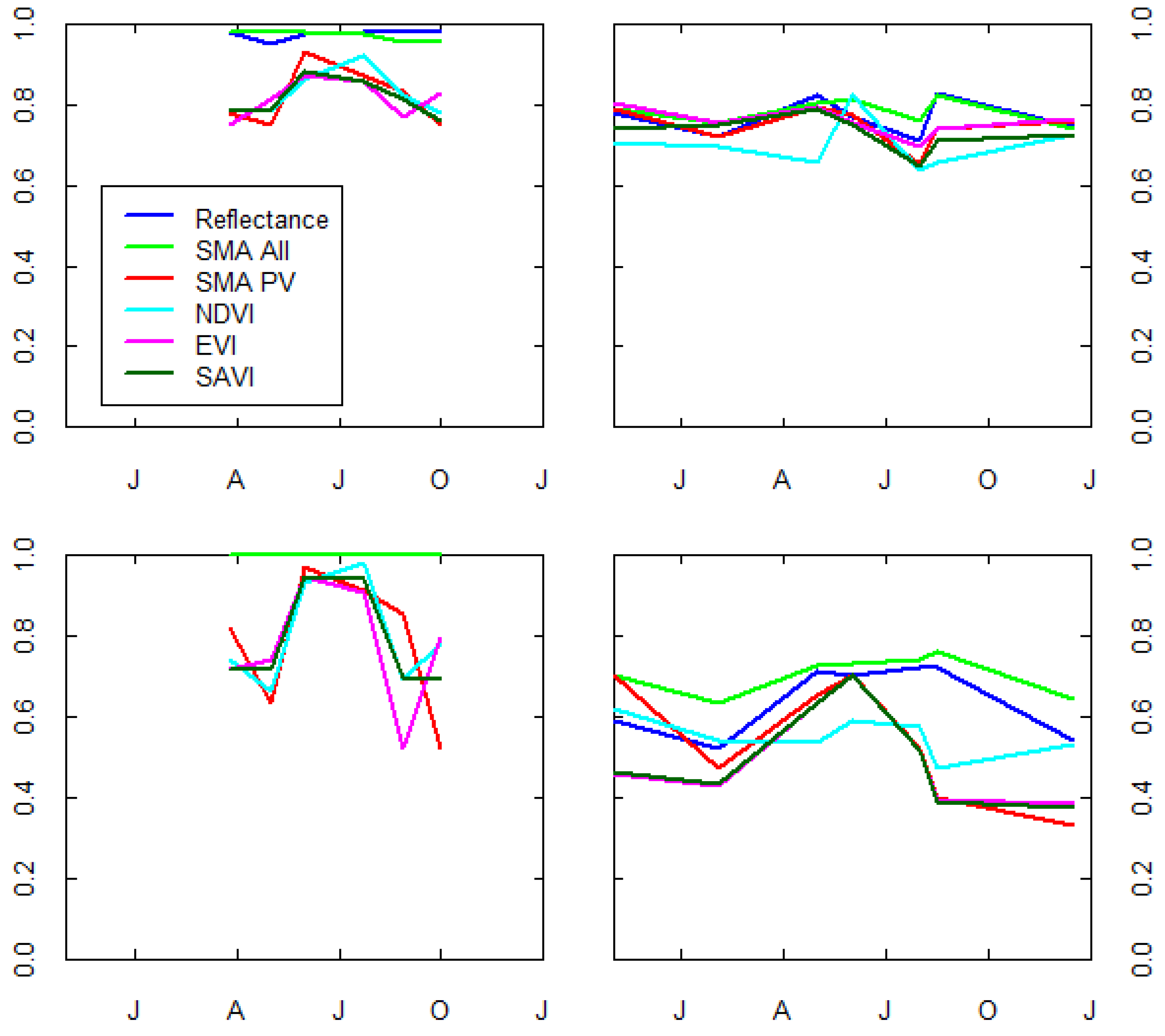
3.2. Mixed Pixel Separability of P. ciliare from Natives in Arizona Upland Landscapes

Predicted reflectance for 6 dates in 2007 of 53 plots used in Olsson et al.’s [15] diversity study are given in Figure 7. This time series captures spring landscape green-up (March–April) followed by an arid fore-summer (May). The onset of the North American monsoon represents the greatest magnitude change in all seasons (May–August). Photosynthetic activity is declining by 22 September and by 26 October, reflectance values are similar to the initial March reflectance values. Wavelengths for which reflectance of dense plots (≥50% P. ciliare) had significantly different reflectance than medium (5–50%) plots are indicated with a full light gray background. Wavelengths for which reflectance of dense plots was different than light (<5%) plots but not medium plots are indicated by a gray background of only half the height of the figure.

Figure 7. Mean simulated reflectance of densely infested (≥50% P. ciliare), moderately infested (5–50% P. ciliare) and uninfested (<5% P. ciliare) plots used in study by Olsson et al. [15]. Wavelengths for which reflectance in densely infested plots are significantly different than in moderately infested and uninfested plots are indicated by full height and half-height grey background, respectively.

Figure 7. Mean simulated reflectance of densely infested (≥50% P. ciliare), moderately infested (5–50% P. ciliare) and uninfested (<5% P. ciliare) plots used in study by Olsson et al. [15]. Wavelengths for which reflectance in densely infested plots are significantly different than in moderately infested and uninfested plots are indicated by full height and half-height grey background, respectively.

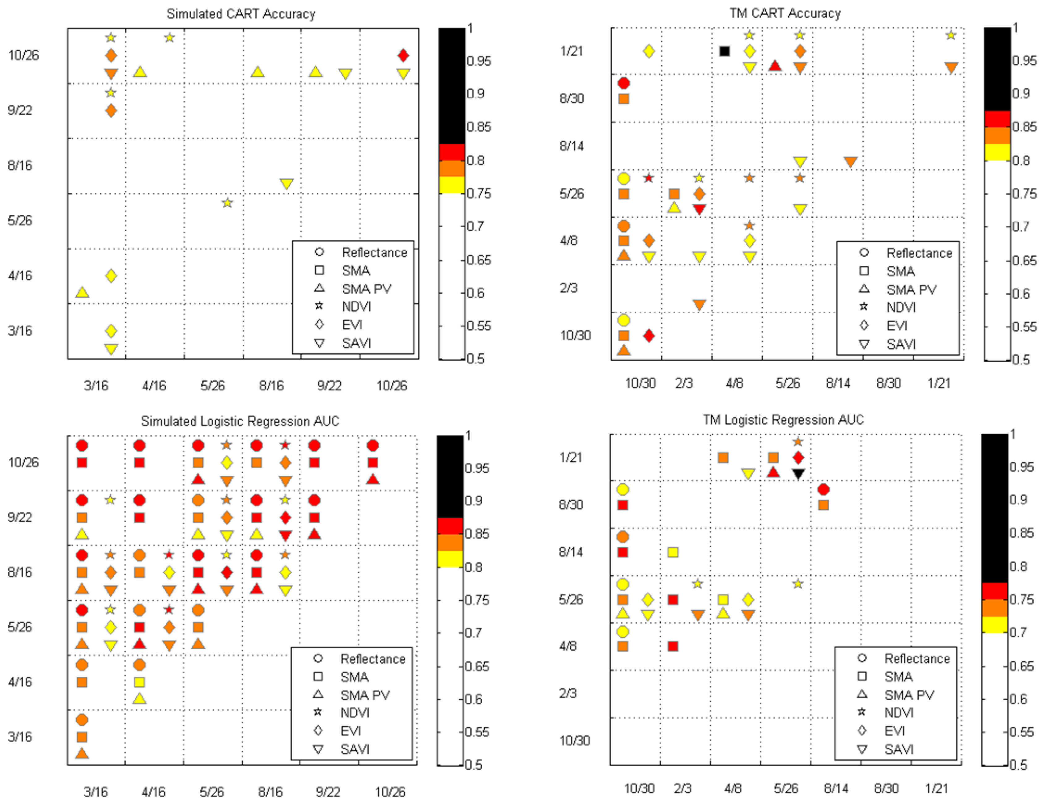
3.3. Single Date Results

P. ciliare-dominated plots differ in their response to the changing seasons in: (1) lower reflectance in the blue wavelength range (400 nm) for all dates, (2) higher red (670 nm) reflectance in April, August, and October, but especially so in August, (3) lower overall reflectance in August, and (4) a more pronounced absorption feature at 2,100 nm in March, May, September and October.

Mean NDVI for training pixels from real Landsat TM scenes are given in Figure 8. Disregarding golf course, riparian, and forest classes, P. ciliare alone had higher mean NDVI than desert scrub in October. In April and May, NDVI was lower, but P. ciliare responded to monsoon precipitation by 8/14 with higher mean NDVI than desert scrub. This was short-lived, as 16 days later the means were identical. By 1/21/08, P. ciliare mean NDVI had dropped below that of desert scrub. This distinction did not translate to classification results.

Figure 8. Mean Normalized difference vegetation index (NDVI) values of training points based on Landsat-5 TM scenes from seven dates over 15 months between 2006 and 2008.

Figure 8. Mean Normalized difference vegetation index (NDVI) values of training points based on Landsat-5 TM scenes from seven dates over 15 months between 2006 and 2008.

CART classification accuracy and logistic regression AUC values for simulated and real Landsat TM scenes are given in Figure 9. Overall accuracy and AUC values were higher in the simulated scenes and, of those models, accuracy and AUC were much higher for the Reflectance model and SMA_All model for all dates. These two models, which had six bands and three bands, respectively, were also highest or among the highest in all dates according to the AUC results, although the accuracy results are less clear. SMA_All and Reflectance for real Landsat TM scenes were the highest in April (4/8) and both August dates (8/16 and 8/30) and were among the leaders of all dates. The simulated Landsat TM classifications exhibited a fairly consistent bell-shaped pattern over the course of the year, starting off either stable or slightly dropping to April, then increasing to May and decreasing after August. Among the VIs of the real Landsat TM scenes, 8/16 NDVI had the highest accuracy and 5/29 PV had the highest AUC. Most classifications had minima on 9/22 and 4/16. The bell-shaped curve seen in the simulated data was not mirrored in the classification of the real Landsat TM data. Although a bell-curve was apparent in the AUCs (PV, EVI, and SAVI) of real Landsat TM models, the peak was shifted towards earlier months; the early season minimum occurred on 2/3 and the late season decline of AUC had occurred by 8/14 whereas the AUC from simulated scenes did not start to decline until late August. Other differences included a dip in accuracy on 8/14 with a rapid rise by 8/30 in all models. Again, the NDVI stood out from the other VIs, displaying later and higher peak accuracy than other VIs.

Figure 9. Classification and regression tree (CART) classification accuracy (top row) and AUC values of logistic regression model (bottom) of simulated Landsat TM scenes (left column) and real Landsat TM scenes (right column). The classifications were based on the original 6 Landsat TM bands (Reflectance), the Spectral mixture analysis (SMA)-derived fractions of Photosynthetic vegetation (PV), non-photosynthetic vegetation (NPV), and NPV (SMA All), the SMA-derived fraction of vegetation (SMA Vegetation), and the vegetation indices, Normalized Vegetation Difference Index (NDVI), Enhanced Vegetation Index (EVI), and Soil-adjusted Vegetation Index (SAVI). The baseline y-axis values for accuracy have been shifted to 0.5 to show greater detail. A grey line on the AUC plots denote the 0.5 line, which represents the point where models are no better than random.

Figure 9. Classification and regression tree (CART) classification accuracy (top row) and AUC values of logistic regression model (bottom) of simulated Landsat TM scenes (left column) and real Landsat TM scenes (right column). The classifications were based on the original 6 Landsat TM bands (Reflectance), the Spectral mixture analysis (SMA)-derived fractions of Photosynthetic vegetation (PV), non-photosynthetic vegetation (NPV), and NPV (SMA All), the SMA-derived fraction of vegetation (SMA Vegetation), and the vegetation indices, Normalized Vegetation Difference Index (NDVI), Enhanced Vegetation Index (EVI), and Soil-adjusted Vegetation Index (SAVI). The baseline y-axis values for accuracy have been shifted to 0.5 to show greater detail. A grey line on the AUC plots denote the 0.5 line, which represents the point where models are no better than random.

3.4. Multidate Results

CART classification accuracy and logistic regression AUC values for two-date combinations of simulated and real Landsat TM scenes are given for the top models in Figure 10. Based on the most accurate models, the dates 26 October and 16 March were included most often in classifications of the simulated TM scenes while 30 October and 21 January were included most often in the classifications of real TM scenes. Based on the models with the highest AUC, the date 16 August from the simulated models and 26 May and 21 January were most often included. The best overall date-combinations in terms of CART model accuracy and logistic regression AUC for simulated scenes were from 26 October + 16 March (accuracy < 0.775) and 26 May + 16 August (AUC < 0.85). Notably, the most accurate CART model involved just the single date of 26 October (accuracy < 0.80). The best models for real TM scenes were from 8 April + 21 January (CART model accuracy > 0.875) and 21 January + 14 August (AUC > 0.775).

Figure 10. CART classification accuracy (top row) and logistic regression AUC (bottom row) of two-scene models for all date combinations using simulated (left column) and real Landsat TM data (right column). Each pixel represents the suite of models developed using the dates denoted by the column and row. Model types are Reflectance (o), SMA (square), SMA PV (triangle), NDVI (star), EVI (diamond), and SAVI (+). Accuracy and AUC are denoted by the color level. Note that axes differ between plots because of different acquisition dates, as do color levels due to large overall differences in accuracy and AUC between simulated and real TM classifications.

Figure 10. CART classification accuracy (top row) and logistic regression AUC (bottom row) of two-scene models for all date combinations using simulated (left column) and real Landsat TM data (right column). Each pixel represents the suite of models developed using the dates denoted by the column and row. Model types are Reflectance (o), SMA (square), SMA PV (triangle), NDVI (star), EVI (diamond), and SAVI (+). Accuracy and AUC are denoted by the color level. Note that axes differ between plots because of different acquisition dates, as do color levels due to large overall differences in accuracy and AUC between simulated and real TM classifications.

Given the number of times each type of model showed up in the top models, vegetation-based classifications were more accurate than SMA or reflectance-based models but the same was not true for AUC. SAVI was more prevalent than other VIs in top models of both simulated and real TM scenes. SAVI was also the basis for the most discriminatory model in the real TM classifications.

While classification accuracy was high, it was disproportionately high considering that 90% of validation points included negative samples. This is conveyed by a 25.7% True Positive Rate and a 74.3% False Negative Rate for the top model overall (1/21 + 4/8 SMA).

4. Discussion

P. ciliare alters ecosystem structure, converting sparse, heterogeneous desert scrub ecosystems characterized by 10–25% cover into well-connected grassland grasslands supporting over 60% cover [11,15]. Several studies hypothesized that such a drastic transformation would be detectable using moderate resolution multispectral sensors such as Landsat TM but were unable to accurately do so [8,9,10]. By analyzing hyperspectral reflectance of P. ciliare and other native cover types, we determined that its spectral reflectance differs from dominant native cover types at different wavelengths at different times of the year, but when present in mixed quantities is difficult to distinguish, especially when reflectance is convolved to TM reflectance in which small-scale variations in spectral response are lost. Four distinguishing spectral features were found in the hyperspectral reflectance curves: (1) cellulose absorption feature at 2,100 nm was seen in P. ciliare at times of the year when this was absent from other vegetation, (2) P. ciliare exhibited higher red reflectance and lower yellow reflectance during senesced phases when contrasted with natives, (3) SWIR2 reflectance rose more rapidly following monsoon precipitation in P. ciliare than native vegetation, and (4) P. ciliare was easily distinguishable from soil, rock, and NPV during spring and summer growing seasons by the presence of vegetative spectral characteristics (e.g., absorption at 670 nm and a steep slope [red edge] from 670 to 800 nm). Landsat TM is unable to resolve the cellulose feature, but with its VNIR bands should be able to resolve the latter three features. Pairing scenes from different seasons in a multi-temporal analysis may increase accuracy over single scenes, but the best models overall were derived from an October TM scene using both simulated and real Landsat TM reflectance. Models based on vegetation indices or unmixed vegetation were as accurate as models based on all six TM bands, indicating that spectral differences in the VNIR are as discriminating as those in the SWIR, or even that the TM SWIR bands add little discriminating power. This result is consistent with personal observations of high contrast between P. ciliare and natives following complete senescence in October and November as shown in Figure 1.

Landsat TM-based classification accuracy was low for both simulated and real TM scenes. We utilized linear (logistic regression) and nonlinear (CART) classification methods with similarly poor results. Nevertheless, we found a number of patterns that have important implications for ecosystem function or can be used to improve the quality of remote sensing results using Landsat TM or other sensors.

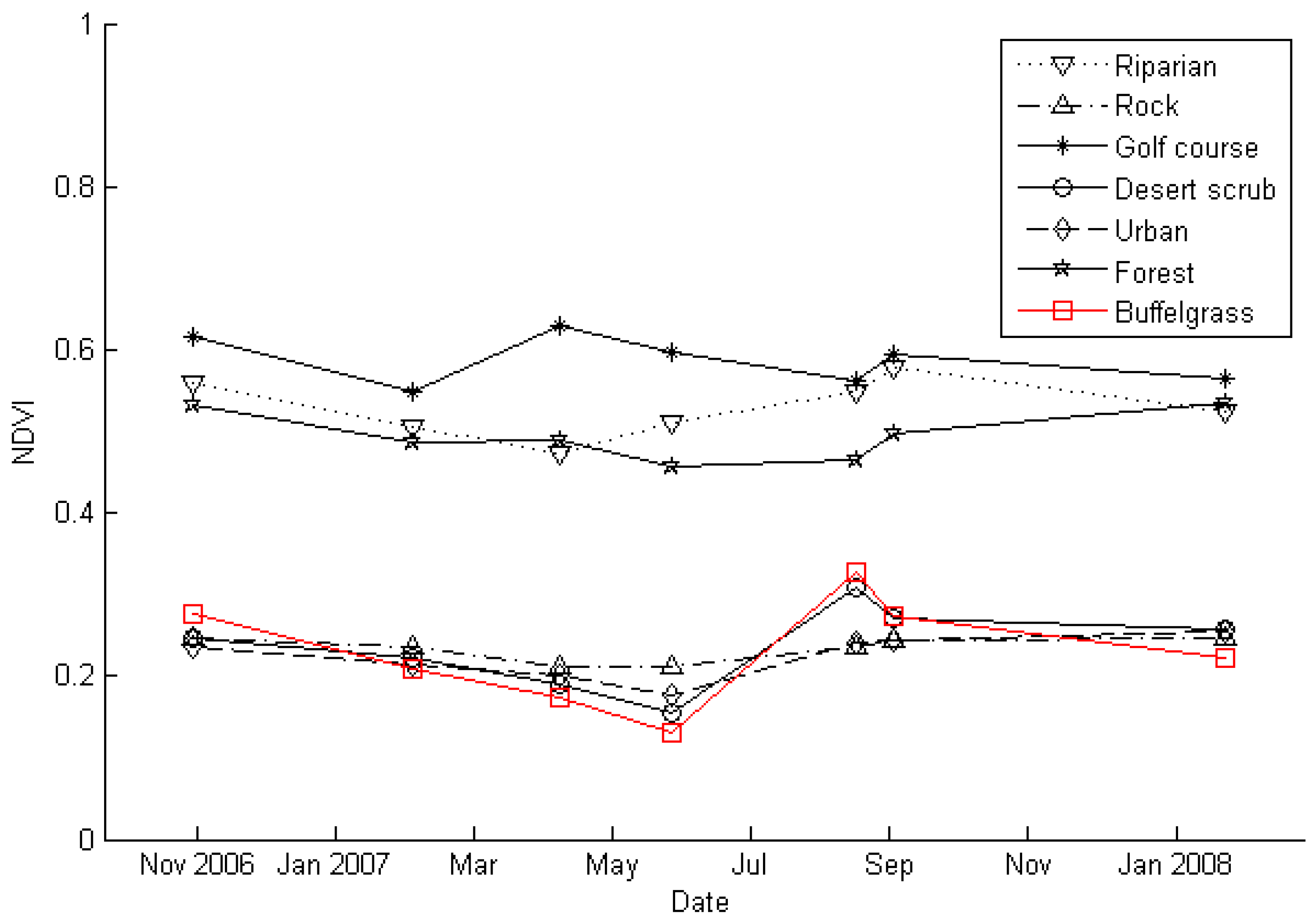
4.1. Invaded Areas are Greener than Uninvaded Areas

Using the spectral model and cover estimates as a foundation for mixture modeling, we found that invaded plots have higher greenness during peak monsoon growth. This is mostly accounted for by differences in vegetative cover between invaded (>70% vegetative cover) and uninvaded (<40%) plots and is highlighted by higher NDVI values in P. ciliare plots in August (Figure 8). However, our multi-temporal mixture model assumed constant cover throughout the year. This may have been more robust for P. ciliare than bare soil because many organisms increase coverage over bare soil in response to summer precipitation. A notable example, the desiccation-tolerant pteridophytes, Selaginella spp., occupy virtually no cover throughout the year but rehydrate and expand to cover a substantial fraction of soil and rock following summer and winter rains (personal observation).

4.2. P. ciliare Dries out and Senesces before Native Vegetation

Warm-season perennial and annual plants in the Sonoran Desert respond vigorously to the onset of monsoon rains and P. ciliare is no exception. However, it appears that P. ciliare dries out earlier than native vegetation as evidenced by the rising reflectance in SWIR1 and SWIR2 in September. The absorption feature at 2,100 nm in September is characteristic of cellulose absorption and likely due to the standing senesced biomass. Additionally, the reduction in absorption at 670 nm in September, which resulted in a yellowish hue, indicated that photosynthetic rate has slowed. This continued into late October when P. ciliare was fully senesced and native vegetation was not yet fully dormant.

4.3. Invaded Areas are Redder during the Senesced Phase

Invaded plots had lower reflectance values than uninvaded plots at 450 nm on all dates. The difference was largest during August and September and smallest during May and April. This separation is due in part to the higher VNIR reflectance associated with soils, rock, and Encelia farinosa, which together account for >60% mean cover in the uninvaded plots. Although VNIR reflectance of P. ciliare closely resembled P. microphylla during peak monsoon growth, it had a distinct shape that contrasted with both P. microphylla and E. farinosa on all five other dates. Differences in the VNIR were further enhanced in September and October, as at 670 nm where reflectance in invaded plots became brighter than uninvaded plots, creating a steeper slope from 450 nm to 700 nm in invaded plots. This translates to a yellow-orange color characteristic that contrasts with the tan background of desert soils. Unfortunately, this contrast may be short-lived. Furthermore, the authors informally monitored these patches in 2008 and 2009 and found that the distinctive hue seen in October–November 2007 was not reproduced in either year. The 2007 crop of P. ciliare was unique over this time period in that 2006 experienced an exceptionally wet summer. By the end of the 2007 growing season, a combination of abundant leaf area resulting from latent stores from 2006 may have combined with climatic events in the fall of 2007 that cured P. ciliare to produce this unique hue. While this may be the case, the October 2006 date was also implicated in higher classification accuracy using real Landsat TM data.

4.4. Best Dates for Distinguishing P. ciliare from Native Vegetation

Late October was the best or second best time of year in terms of CART classification accuracy and logistic regression class discrimination for both simulated and real Landsat TM scenes. In addition, CART models based on 26 October (simulated) and 30 October (real TM) produced models that were comparable to the multidate models. Late May also produced a number of good models using real Landsat TM scenes. The likely explanation is lower photosynthetic rates in P. ciliare-dominated pixels than uninvaded pixels as shown in Figure 8. P. microphylla and other desert natives maintain photosynthesis throughout the summer, albeit at low levels; whereas, P. ciliare does not. Where P. ciliare has displaced these natives, ecosystem photosynthesis is likely depressed. Interestingly, combinations of May and October were not as accurate or discriminatory as other combinations of May, notably May + January and May + February. We did not acquire hyperspectral reflectance during the months of January or February so it is unclear what the mechanisms may be, although a phenological contrast is likely. The months of January and February (winter scenes) were only highlighted by good models when combined with April or May (summer dry scenes). We pose several untested hypotheses: (1) P. ciliare cover competitively inhibits winter annual plants and drought-desiccant mosses, (2) P. ciliare greens up in response to winter precipitation earlier than natives. Either explanation would account for slight changes in both seasons that would be amplified when compared in tandem. The dates predicted by simulated scenes that were not effective discriminating dates in real Landsat TM scenes were the August dates (peak monsoon scenes). This may be due to an oversimplification of the landscape. By not accounting for replacement of bare soil and rock by summer annuals, drought-desiccant mosses, and biological crusts, we overestimated the role that interstitial spaces would play in distinguishing invaded landscapes from uninvaded desert scrub. Considering this, it is worth noting that the few good models produced from August scenes were multi-date models including the scene immediately prior (May) or after (October). We have discussed the benefits of using May and October scenes, but this result lends support to the hypothesis that P. ciliare invasion alters ecosystem function, changing the magnitude of phenological change.

5. Concluding Remarks

We developed and tested a new method for assessing the feasibility of detecting sub-pixel land cover differences in highly mixed pixels that utilizes ground-based reflectance and cover measurements over time. By recombining endmembers in fractions derived from distributions of real-world samples, the optimal timing of separation between invaded and uninvaded pixels can be predicted for various sensors. We selected Landsat TM both to explain past failures to detect P. ciliare in the Sonoran Desert and to identify optimum timing for accurately discriminating between P. ciliare and uninvaded pixels. We note some shortcomings of this approach, mostly arising due to a simplification of the simulated landscape. This could be overcome by improving the land cover model to account for seasonal changes in canopy cover.

Our results show that, although P. ciliare is distinguishable from uninvaded areas in many portions of the electromagnetic spectrum, Landsat TM-based reflectance differences of uninvaded and invaded landscapes are minimal due to the high level of mixing. While classification can be improved by strategically selecting scenes with better phenological distinctions (e.g., late October and May), classification accuracy is remarkably low. Due to the disproportionate role that small, remote outbreaks play in the spread of invasive species, it is unlikely that Landsat TM is going to be able to play an operational role in the detection and monitoring of P. ciliare in the mixed scrub habitats of the Sonoran Desert. The TM sensor lacks the spatial resolution to isolate pure P. ciliare pixels and the spectral resolution to identify the distinctive cellulose absorption characteristic of senesced P. ciliare. An operational method would need to address one or both of these issues. Although the shape of visual reflectance distinguished invasive from uninvaded plots in our study area, the narrow range of values limited by a three- or four-band scene is likely to result in confusion. We feel that a sensor with narrow bands at 2,050 nm, 2,100 nm, and 2,150 nm would be essential.

References

- D’Antonio, C.M.; Vitousek, P.M. Biological invasions by exotic grasses, the grass fire cycle, and global change. Ann. Rev. Ecol. Syst. 1992, 23, 63–87. [Google Scholar] [CrossRef]
- Brooks, M.L.; D’Antonio, C.M.; Richardson, D.M.; Grace, J.B.; Keeley, J.E.; DiTomaso, J.M.; Hobbs, R.J.; Pellant, M.; Pyke, D. Effects of invasive alien plants on fire regimes. Bioscience 2004, 54, 677–688. [Google Scholar] [CrossRef]
- Mclaughlin, S.P.; Bowers, J.E. Effects of wildfire on a Sonoran Desert plant community. Ecology 1982, 63, 246–248. [Google Scholar] [CrossRef]
- Burquez-Montijo, A.M.; Miller, M.E.; Yrizar, A.M.; Tellman, B. Mexican grasslands, thornscrub, and the transformation of the Sonoran Desert b invasive exotic buffelgrass (Pennisetum ciliare). In Invasive Exotic Species in the Sonoran Region; Tellman, B., Ed.; The University of Arizona Press-The Arizona-Sonora Desert Museum: Tucson, AZ, USA, 2002; pp. 126–146. [Google Scholar]
- Williams, D.G.; Baruch, Z. African grass invasion in the Americas: Ecosystem consequences and the role of ecophysiology. Biol. Invasions 2000, 2, 123–130. [Google Scholar] [CrossRef]
- Van Devender, T.R.; Felger, R.S.; Burquez-Montijo, A. Exotic Plants in the Sonoran Desert Region, Arizona and Sonora. In Proceedings of the California Exotic Pest Plant Council Symposium, Concord, CA, USA, 11 December 1997; Volume 3, pp. 10–15.
- Rogstad, A. The Buffelgrass Strategic Plan; Arizona-Sonora Desert Museum: Tucson, AZ, USA, 2008. [Google Scholar]
- Brenner, J. Structure, Agency, and the Transformation of the Sonoran Desert by Buffelgrass (Pennisetum ciliare): An Application of Land Change Science. Ph.D. Thesis, Clark University, Worcester, MA, USA, 2009. [Google Scholar]
- Franklin, K.A.; Lyons, K.; Nagler, P.L.; Lampkin, D.; Glenn, E.P.; Molina-Freaner, F.; Markow, T.; Huete, A.R. Buffelgrass (Pennisetum ciliare) land conversion and productivity in the plains of Sonora, Mexico. Biol. Conser. 2006, 127, 62–71. [Google Scholar] [CrossRef]
- Olsson, A.D.; Marsh, S.E.; Orr, B.J.; Guertin, D.P. Development of a Spatial Decision Support System for Buffelgrass Management for the Tucson Mountain Sector of Pima County; Pima County Natural Resources Parks and Recreation: Tucson, AZ, USA, 2009. [Google Scholar]
- Turner, R.M.; Brown, D.E. Sonoran Desert scrub. In Biotic Communities: Southwestern United States and Northwestern Mexico; Brown, D.E., Ed.; University of Utah Press: Salt Lake, UT, USA, 1994; pp. 181–221. [Google Scholar]
- Huete, A.R. A Soil-Adjusted Vegetation Index (SAVI). Remote Sens. Environ. 1988, 25, 295–309. [Google Scholar] [CrossRef]
- Shreve, F.; Wiggins, I.L. Vegetation and Flora of the Sonoran Desert; Stanford University Press: Stanford, CA, USA, 1964. [Google Scholar]
- de la Fuente, E.G.; Solis, J.D.; Fitzmaurice, A.S.; Encinia, F.B.; Tristan, V.V.; Grant, W.E. Growth rate pattern of buffelgrass [Pennisetum ciliare L. (Link.) Syn. Cenchrus ciliaris L.] in Tamaulipas, Mexico. Tecnica Pecuaria En Mexico 2007, 45, 1–17. [Google Scholar]
- Olsson, A.D.; McClaran, M.P.; Marsh, S.E. Transformation rate and extent of undisturbed Sonoran desert scrub by invasive buffelgrass. Biol. Invasions 2011. in review. [Google Scholar]
- Moody, M.E.; Mack, R.N. Controlling the spread of plant invasions—The importance of Nascent Foci. J. Appl. Ecol. 1988, 25, 1009–1021. [Google Scholar] [CrossRef]
- Daughtry, C.S.T. Discriminating crop residues from soil by shortwave infrared reflectance. Agron. J. 2001, 93, 125–131. [Google Scholar] [CrossRef]
- Tucker, C.J. Red and photographic infrared linear combinations for monitoring vegetation. Remote Sens. Environ. 1979, 8, 127–150. [Google Scholar] [CrossRef]
- Jackson, R.D.; Slater, P.N.; Pinter, P.J. Discrimination of growth and water-stress in wheat by various vegetation indexes through clear and turbid atmospheres. Remote Sens. Environ. 1983, 13, 187–208. [Google Scholar] [CrossRef]
- Tucker, C.J.; Newcomb, W.W.; Los, S.O.; Prince, S.D. Mean and inter-year variation of growing-season Normalized Difference Vegetation Index for the Sahel 1981–1989. Int. J. Remote Sens. 1991, 12, 1133–1135. [Google Scholar] [CrossRef]
- WRCC. Arizona Climate Summaries; Western Regional Climate Center: Reno, NV, USA, 2010. [Google Scholar]
- Lowry, J.; Ramsey, R.D.; Thomas, K.; Schrupp, D.; Sajwaj, T.; Kirby, J.; Waller, E.; Schrader, S.; Falzarano, S.; Langs, L.; et al. Mapping moderate-scale land-cover over very large geographic areas within a collaborative framework: A case study of the Southwest Regional Gap Analysis Project (SWReGAP). Remote Sens. Environ. 2007, 108, 59–73. [Google Scholar] [CrossRef]
- Bowers, J.E.; Bean, T.; Turner, R.M. Two decades of change in distribution of plants at the desert laboratory, Tucson, Arizona. Madrono 2006, 53, 252–263. [Google Scholar] [CrossRef]
- Chavez, P.S. Image-based atmospheric corrections revisited and improved. Photogramm. Eng. Remote Sensing 1996, 62, 1025–1036. [Google Scholar]
- Beyer, H.L. Hawth’s Analysis Tools v 3.27 for ArcGIS 9.x. 2004. Available online: http://www.spatialecology.com/htools (accessed on 13 October 2011).
- Vermote, E.F.; Tanre, D.; Deuze, J.L.; Herman, M.; Morcrette, J.J. Second Simulation of the Satellite Signal in the Solar Spectrum, 6S: An overview. IEEE Trans. Geosci. Remote Sens. 1997, 35, 675–686. [Google Scholar] [CrossRef]
- Adams, J.B.; Smith, M.O. Spectral mixture modeling: A new analysis of rock and soil types at the Viking lander 1 suite. J. Geophys. Res. 1986, 91, 8098–8112. [Google Scholar] [CrossRef]
- Penrose, R.; Todd, J.A. On best approximate solution of linear matrix equations. Math. Proc. Cambridge Phil. Soc. 1956, 52, 17–19. [Google Scholar] [CrossRef]
- Huete, A.; Didan, K.; Miura, T.; Rodriguez, E.P.; Gao, X.; Ferreira, L.G. Overview of the radiometric and biophysical performance of the MODIS vegetation indices. Remote Sens. Environ. 2002, 83, 195–213. [Google Scholar] [CrossRef]
- Breiman, L. Classification and Regression Trees; Wadsworth International Group: Belmont, CA, USA, 1984. [Google Scholar]
- Ramsey, F.L.; Schafer, D.W. The Statistical Sleuth: A Course in Methods of Data Analysis, 2nd ed.; Duxbury Press: Pacific Grove, CA, USA, 2002. [Google Scholar]
- Fielding, A.H.; Bell, J.F. A review of methods for the assessment of prediction errors in conservation presence/absence models. Environ. Conser. 1997, 24, 38–49. [Google Scholar] [CrossRef]
© 2011 by the authors; licensee MDPI, Basel, Switzerland. This article is an open access article distributed under the terms and conditions of the Creative Commons Attribution license (http://creativecommons.org/licenses/by/3.0/).
Share and Cite
Olsson, A.D.; Van Leeuwen, W.J.D.; Marsh, S.E. Feasibility of Invasive Grass Detection in a Desertscrub Community Using Hyperspectral Field Measurements and Landsat TM Imagery. Remote Sens. 2011, 3, 2283-2304. https://0-doi-org.brum.beds.ac.uk/10.3390/rs3102283
Olsson AD, Van Leeuwen WJD, Marsh SE. Feasibility of Invasive Grass Detection in a Desertscrub Community Using Hyperspectral Field Measurements and Landsat TM Imagery. Remote Sensing. 2011; 3(10):2283-2304. https://0-doi-org.brum.beds.ac.uk/10.3390/rs3102283
Chicago/Turabian StyleOlsson, Aaryn D., Willem J.D. Van Leeuwen, and Stuart E. Marsh. 2011. "Feasibility of Invasive Grass Detection in a Desertscrub Community Using Hyperspectral Field Measurements and Landsat TM Imagery" Remote Sensing 3, no. 10: 2283-2304. https://0-doi-org.brum.beds.ac.uk/10.3390/rs3102283