Spaceborne Differential SAR Interferometry: Data Analysis Tools for Deformation Measurement

Abstract

This paper is focused on spaceborne Differential Interferometric SAR (DInSAR) for land deformation measurement and monitoring. In the last two decades several DInSAR data analysis procedures have been proposed. The objective of this paper is to describe the DInSAR data processing and analysis tools developed at the Institute of Geomatics in almost ten years of research activities. Four main DInSAR analysis procedures are described, which range from the standard DInSAR analysis based on a single interferogram to more advanced Persistent Scatterer Interferometry (PSI) approaches. These different procedures guarantee a sufficient flexibility in DInSAR data processing. In order to provide a technical insight into these analysis procedures, a whole section discusses their main data processing and analysis steps, especially those needed in PSI analyses. A specific section is devoted to the core of our PSI analysis tools: the so-called 2+1D phase unwrapping procedure, which couples a 2D phase unwrapping, performed interferogram-wise, with a kind of 1D phase unwrapping along time, performed pixel-wise. In the last part of the paper, some examples of DInSAR results are discussed, which were derived by standard DInSAR or PSI analyses. Most of these results were derived from X-band SAR data coming from the TerraSAR-X and CosmoSkyMed sensors.

1. Introduction

Spaceborne differential interferometric SAR (DInSAR) dates back to 1989 when a technique that exploited L-band SEASAT SAR data was first described [1]. Within DInSAR, the most advanced methods that make use of large sets of SAR images date back more than a decade. In particular, Persistent Scatterer Interferometry (PSI) techniques were first published in the article by Ferretti and co-authors [2]. For a general review of SAR interferometry see [3]. A general review of DInSAR can be found in [4], while a more specific review of PSI applications in urban areas is provided in [5].

During the last two decades, DInSAR has demonstrated its unmatched deformation measurement and monitoring capabilities in a wide range of application fields. An extensive list of successful examples is provided in [3]. However, it is important to underline that DInSAR techniques are not universal, nor robust deformation measurement and monitoring tools. This is largely related to two intrinsic limitations of any DInSAR technique: coherence loss (or lack of Persistent Scatterers—PS) and the need to deal with phase ambiguities or wrapped phases. DInSAR only works if the interferometric phase is good enough to get reliable deformation estimates. The pixels that satisfy this condition are often called coherent pixels or PSs. Regardless of the type of DInSAR technique at hand, coherence loss is the most important limitation of DInSAR, which makes it an “opportunistic deformation measurement method” able to measure deformation only over the available coherent pixels and PSs. The second intrinsic limitation, which affects DInSAR robustness, is related to the ambiguous nature of the DInSAR observations: it suffers severe limitations in the capability to measure “fast” deformation phenomena. For more information on the limitations of the DInSAR techniques, see [5].

Several DInSAR data analysis procedures have been proposed in the last 20 years. Some of them are very simple, like the standard DInSAR configuration, which involves the exploitation of a single interferogram computed from a pair of complex SAR images. Others, like PSI techniques, make use of redundant SAR data and quite refined estimation procedures. In the authors’ opinion, none of the proposed procedures can successfully cover the whole range of potential DInSAR applications (applications where it is indeed possible to make use of DInSAR): this can only be achieved by using different complementary DInSAR methods.

The goal of this paper is to review the experience in DInSAR that the Institute of Geomatics (IG) has gained in almost ten years of research and development activities in this field, often in close cooperation with the Department of Earth Sciences of the University of Milan. In this period, different types of data analysis procedures have been implemented, tested and validated using the spaceborne SAR data acquired by the following sensors: ERS-1 (C-band), ERS-2 (C-band), ASAR-Envisat (C‑band), TerraSAR-X (X-band) and CosmoSkyMed (X-band). In addition, several DInSAR tools have been used to process and analyze C-band and Ku-band data captured by terrestrial SAR sensors [6]. The DInSAR data analysis implemented at the IG is based on flexible tools ranging from the standard DInSAR configuration to an advanced PSI method. A summary of the different types of DInSAR analysis procedures currently used at IG is provided in the next section. Some of the most relevant technical details of these procedures are outlined in Section 3. A specific section is then devoted to the phase unwrapping strategy followed by the IG. Finally, some relevant examples of DInSAR results from very high resolution X-band SAR data are discussed in Section 4.

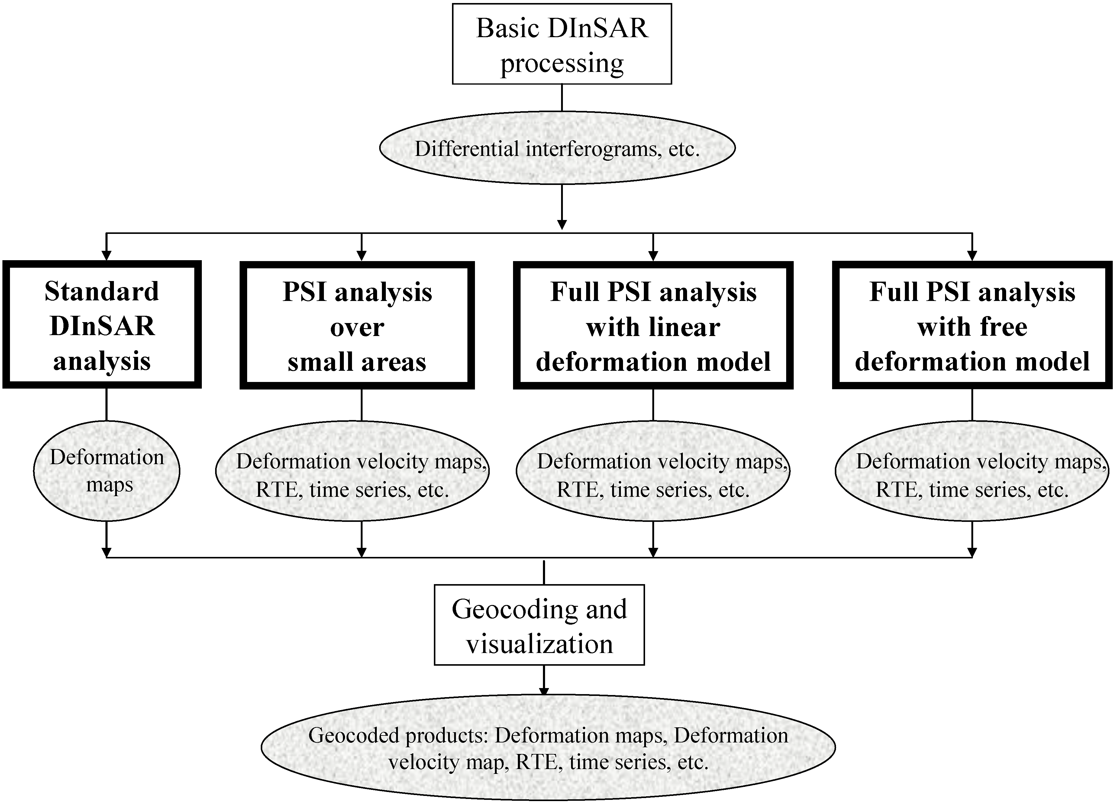
2. DInSAR Analysis Strategies

As mentioned above, the IG is currently implementing different types of DInSAR analysis procedures, see Figure 1. All the procedures share the same initial and final modules: the basic DInSAR processing and the geocoding and visualization. The basic DInSAR processing, usually based on the Diapason software, includes geometric calibration of the master image, image co-registration and interferogram generation. Image calibration, which involves the estimation of the near slant range and the time of acquisition of the first image line, is based on an external Digital Elevation Model (DEM) of the observed area. This step plays a key role in the object-to-image space transformation, used in the differential interferogram generation, and in the image-to-object transformation used in product geocoding. The calibration is followed by image co-registration and the selection of the set of interferograms to be generated. Usually, not all image combinations are exploited: the interferogram set is often chosen by fixing threshold values of the interferogram normal baselines (generally below a few hundred meters) and temporal baselines. Then four different DInSAR data analysis strategies, briefly discussed below, are currently used. A fifth strategy based on a least squares (LS) adjustment and a stepwise linear function for the deformation is described in [7].

Figure 1. General scheme of the different DInSAR data analysis procedures used at IG.

Figure 1. General scheme of the different DInSAR data analysis procedures used at IG.

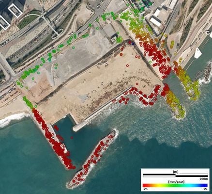
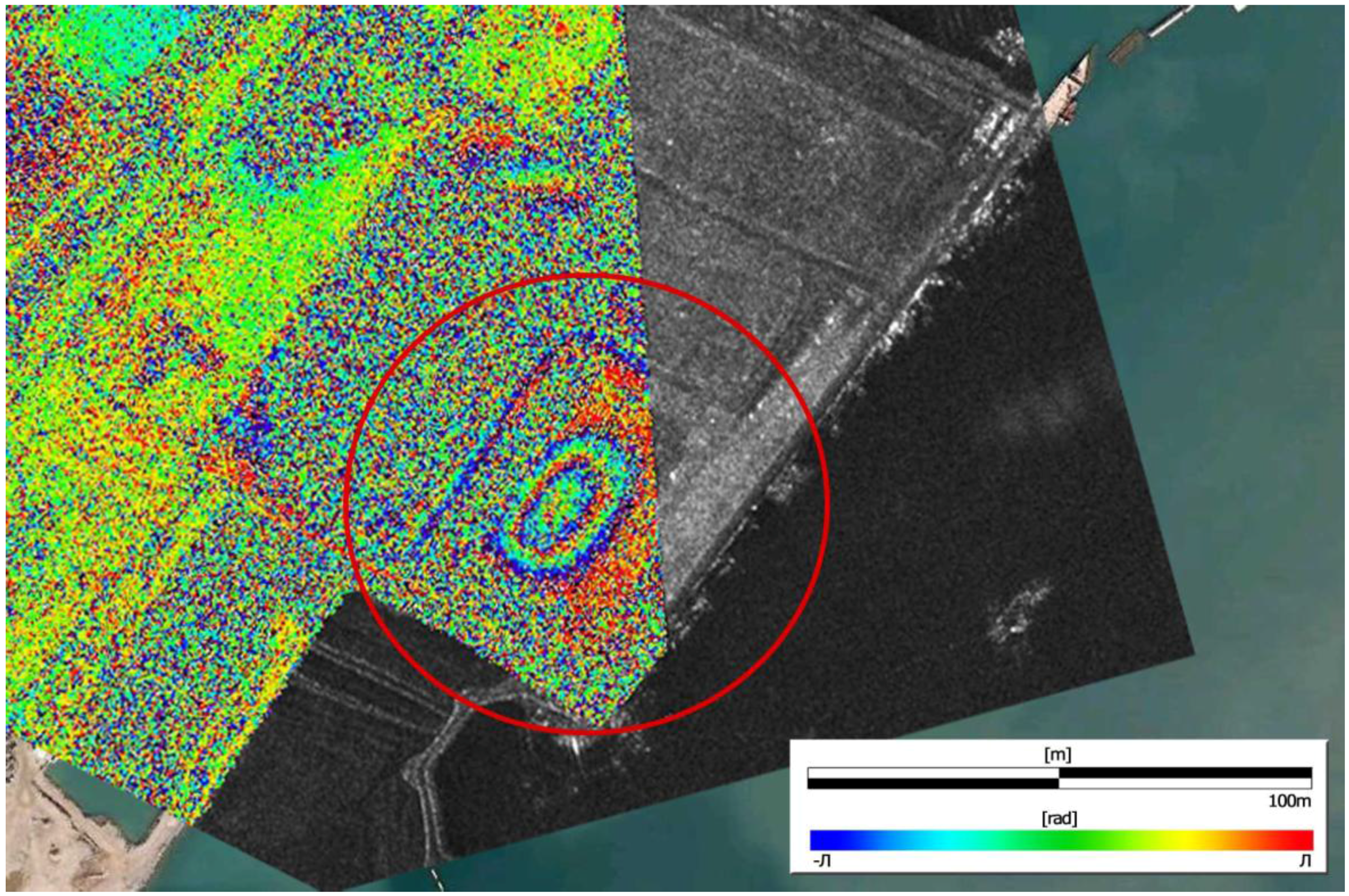
• Standard DInSAR analysis. This simple analysis can be useful to study fast deformation phenomena [8], or displacements occurred in a short period of time when compared to the satellite revisiting time, for example, co-seismic deformation. The best results are achieved using several pairs of interferograms and restricting the analysis to small areas (e.g., up to a few square kilometres), see also [9].
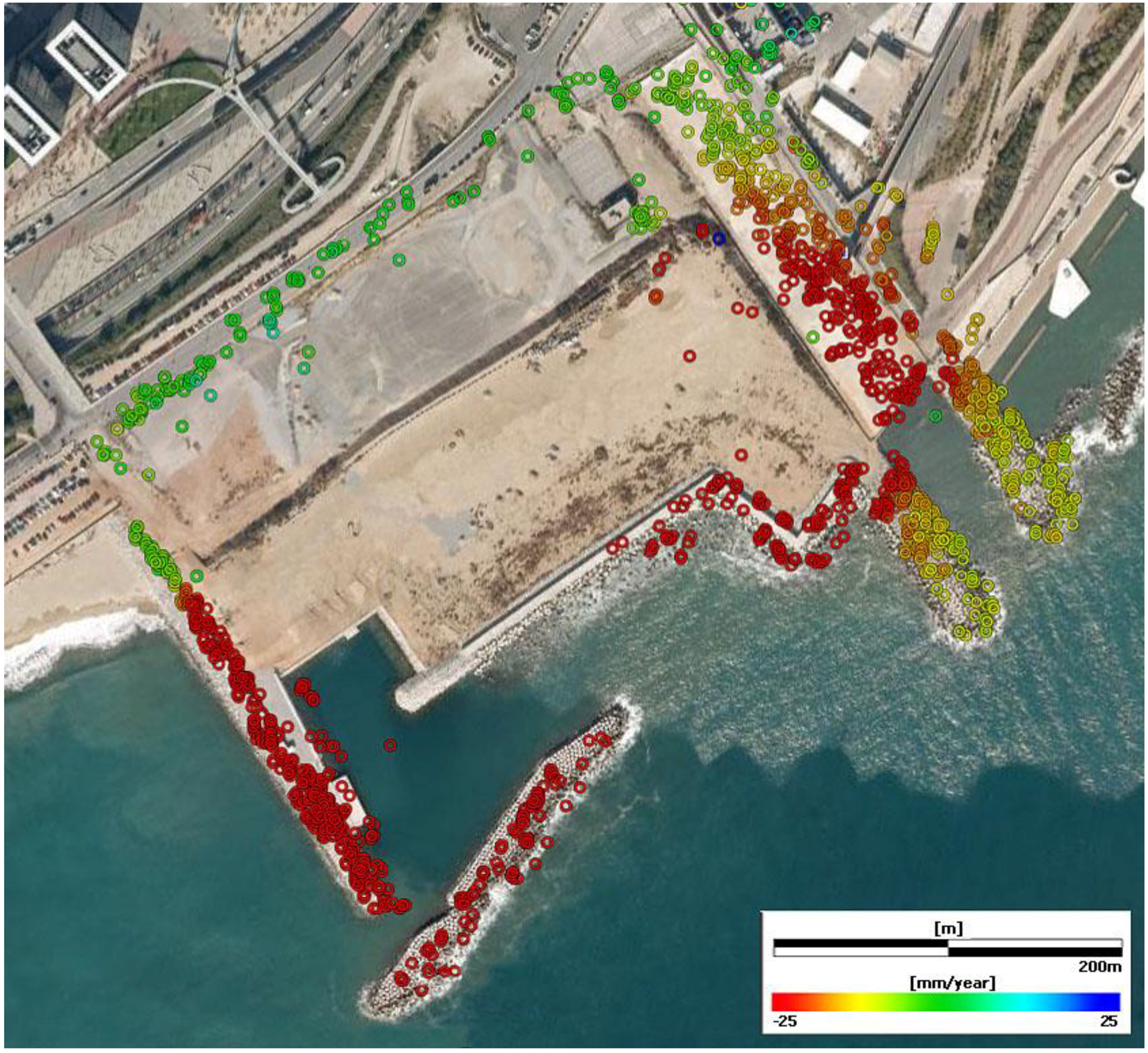
• Small-area PSI analysis. The atmospheric component of DInSAR observations is considerably low in areas up to a few square kilometers. Over small areas, where the atmospheric component has a negligible impact, it is often sufficient to run a simplified PSI data analysis procedure, which does not directly involve the estimation of the atmospheric component. A complete description of this approach, which includes a linear deformation model, is described in [8]. This approach considerably simplifies the computation burden of the analysis and it is by far the approach most commonly used by the authors. The same approach has been recently extended to the estimation of thermal maps (exploiting the thermal expansion component of the PSI observations) using very high resolution X-band SAR data, see [10].
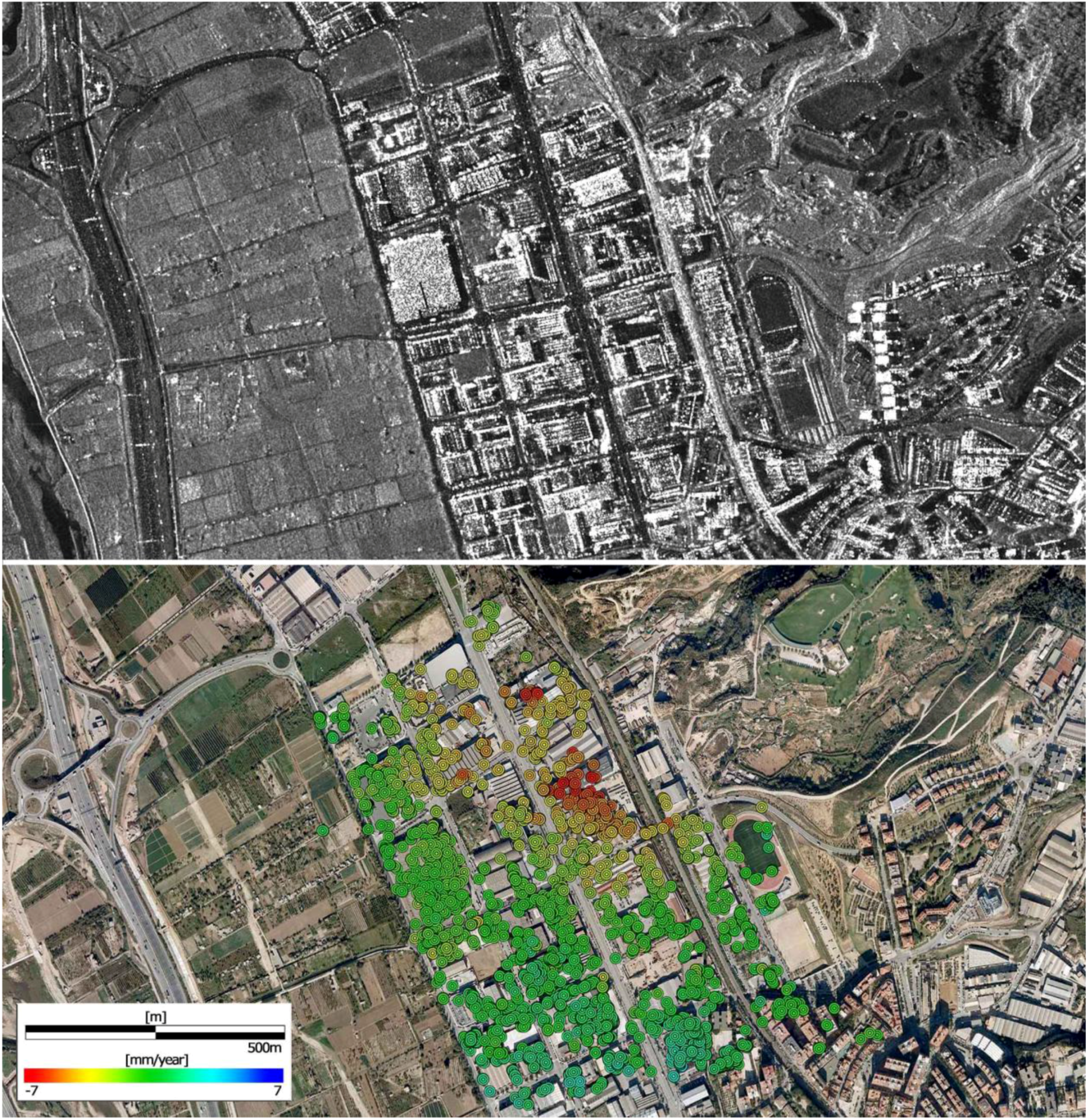
• Full PSI analysis with linear deformation model. This is a standard PSI analysis, which makes use of a linear function to model time deformation evolution. In addition, it separates the atmospheric and deformation components through an appropriate filtering procedure which allows the use of this procedure to analyze wide areas. Several PSI approaches are described in the literature, for example, see [2,11,12,13]. The most important characteristics of the PSI approach implemented at IG are described in the following two sections. It is worth mentioning an important disadvantage of the linear deformation model. This assumption, which is needed to deal with the wrapped interferometric phases, may have a negative impact on deformation estimates for phenomena characterized by non-linear deformation behaviors, that is, where the above assumption is not valid. When the deformation shows “significantly non-linear motion” the PSI procedure “looses” PSs: unfortunately this lack of PSs usually occurs in the areas where the most important deformation phenomena occur. This limitation has to be considered to properly interpret the PSI deformation velocity maps.
• Full PSI analysis with free deformation model. This is the most advanced PSI analysis implemented at IG. In order to avoid the limitation discussed in the previous point, the PSI analysis does not estimate the linear component of deformation. Some of the technical details of this procedure are outlined in the next sections. This approach is useful to analyze deformation phenomena that are highly non-linear in time, for example, the displacements associated with mining activities and tunneling activities, different types of landslides, etc. In addition, this approach is always used to analyze Ground-based SAR (GBSAR) data, which often include very large stacks of SAR images. In fact, especially when continuous GBSAR campaigns are performed, a very dense temporal sampling (with up to one image acquisition every few minutes) and very large stacks (stacks of some thousands of images have been processed at IG) are obtained. In these cases, the free deformation model is used instead of the linear deformation model in order to exploit the valuable information contained in such stacks. It is worth noting that this approach, like all other DInSAR techniques, is limited by the ambiguous nature of the interferometric phases. This issue is discussed later in this paper.

3. Relevant PSI Processing and Analysis Steps

In this section, some of the most relevant steps of the three PSI processing and analysis procedures implemented at IG are described. Each step is briefly outlined below.

• Pixel selection. Like any other PSI technique, the IG procedure exploits only a particular class of pixels, namely coherent pixels or PSs. These points are typically parts of manmade features, such as building and metallic structures, or other natural features like exposed rocks. Pixel selection at full SAR resolution is usually based on the analysis of the SAR amplitude stability over time [14]. The interferometric coherence is used for pixel selection in PSI analyses based on multi-look images (all pixels whose coherence is above a given threshold are selected).
• Estimation of deformation velocity and residual topographic error (RTE). The selected pixels are connected pair-wise by edges, computing the phase difference for each edge and for each of the n interferograms. Redundant connections (i.e., edges) between pixels are used because they provide more robust results than the standard Delaunay triangulation. From the vector of n differential interferometric wrapped phases, using the method of the periodogram, two unknowns per each edge are computed: the differential deformation velocity and the differential RTE. These differential values are then integrated over the whole edge set using an iterative LS procedure. The whole procedure is described in detail in [8], while an extension of the model to account for the thermal expansion, which is particularly important in X-band PSI, is described in [10]. The above procedure is performed if the PSI analysis with linear deformation model is chosen. When the PSI analysis with free deformation model is implemented, the above procedure is only executed for the RTE, fixing to zero the values of the deformation velocity (which in this case is estimated in a later stage).
• Removal of the deformation velocity and RTE phase components. The deformation velocity and RTE values estimated over the pixels selected in the previous step are used to compute the corresponding phase components for each of the n interferograms. Both components are then subtracted from the original interferometric phase, getting a cleaned interferometric phase, which is then processed in the subsequent processing stages. This operation is particularly helpful during phase unwrapping; it is systematically performed for the RTE, especially when processing full resolution data.
• 2+1D phase unwrapping. In this step the interferometric phases are reconstructed by adding integer multiples of 2π to their wrapped values. This operation involves a 2D phase unwrapping, which is run for each interferogram separately using an implementation of the Minimum Cost Flow method [15,16]. The temporal component is then exploited in the so-called “phase estimation” stage, which represents a kind of 1D phase unwrapping along time. For this reason, the entire procedure is named “2+1D phase unwrapping”. Provided that this is the most original part of the whole procedure, it is described in detail in the next section. Its output is a set of phase time series, which contain one sample per each acquisition date of the SAR images, having set to zero the phase of the first image. In other words, the output is a set of m–1 phase images, where m is the number of processed SAR images.
• Estimation of orbital phase trends. Each phase estimated in the previous step contains three main components: deformation, atmospheric contribution and linear trends (tilts) due to orbital errors. The objective of this step is to separate the third component from the other two. This separation is accomplished by exploiting the very smooth spatial pattern caused by orbital errors. This component is estimated by fitting a bilinear polynomial function to each phase images when the study area is approximately smaller than 30 by 30 km. Polynomials of slightly higher order can be used for larger areas.
• Spatio-temporal filtering. After removing the contribution of the orbital errors, each phase contains the deformation and the atmospheric components. A set of filters is then applied to separate the two components. The filters exploit the property described in [2,14]: the atmospheric and the deformation signals have different behavior in time and space. In particular, the atmospheric component is characterized by a high spatial correlation and low temporal correlation. The outcome of this step is the estimated atmospheric contribution (Atmospheric Phase Screen) for each of the m–1 images. The average of all this m–1 contributions is used to estimate the atmospheric contribution of the first image, see [14]. It is worth noting that the deformation time series of the analyzed pixels is also obtained at this stage. However, the final deformation time series are estimated in step 9, which performs a densification with respect to the pixels analyzed in the steps 1–6.
• Atmospheric and orbital error removal. The orbital trends and the atmospheric contributions estimated, for m–1 images, in the previous two steps are then subtracted from the phases of the n interferograms generated at step 3. This operation involves an extrapolation of the atmospheric phase contribution estimated in the previous step to all the image pixels. The interferometric phases cleaned by orbital and atmospheric effects are obtained.
• Pixel densification. The pixel selection described in step 1 is repeated in this step but relaxing the selection thresholds. The objective is to obtain a denser set of pixels, over which the PSI estimation procedure can be performed.
• Estimation of the final products. The final PSI products are generated by running a second iteration of steps 2, 3 and 4 over the denser set of pixels obtained in the previous step. The first product is the RTE map. It is used, internally in the PSI procedure, to geocode the processed PS’s and hence all the PSI products. The use of the RTE generates an advanced geocoding, which is a key step in PSI product exploitation [17]. In addition, since the RTE map provides the height of each PS, it gives fundamental information for the interpretation of the PSI results. The second product is the set of deformation time series. They are generated by adding the deformation velocity that was previously removed from the phases (step 3 of the second processing iteration) to the output of the second iteration of step 4. As described in the next section, the deformation time series are associated with different by-products of the processing step 4, which can be used to assess their quality. Finally, the last product is the deformation velocity map, which is derived by LS fitting to the deformation time series.

The 2+1D Phase Unwrapping Procedure

In this section, the 2+1D phase unwrapping procedure, which represents the most original part of the whole IG PSI processing chain, is described in detail. 2D phase unwrapping is a critical and error‑prone processing stage. Different factors, for example, phase noise, high deformation rates, high local deformation gradients, isolated pixels, etc. can cause errors (that are integer multiples of 2π) during this step. The 2D unwrapping is complemented by the “phase estimation” step, which, starting from the stack of 2D unwrapped differential interferometric phases (the observations), provides pixel‑wise, the phase values in correspondence to each SAR image (the unknown parameters). This is done using an iterative Single Value Decomposition (SVD) LS procedure, see [18,19], and exploiting the integer nature of the 2D unwrapping errors to detect and correct (if possible) these errors or reject the erroneous observations. The main observation equation is given by:

$$\Delta \phi ={({\phi }_{defo}+{\phi }_{atmo}+{\phi }_{tlin})}_S-{({\phi }_{defo}+{\phi }_{atmo}+{\phi }_{tlin})}_M+2N\cdot \pi +{\phi }_{res}$$

(1)

where $\Delta \phi$ is the 2D unwrapped interferometric phase (the observation), S and M are the slave and master images respectively, ${\phi }_{defo}$ is the phase component due to deformation, ${\phi }_{atmo}$ is the term due to atmospheric effects, ${\phi }_{tlin}$ is the term due to orbital errors, $N$ is an integer number and ${\phi }_{res}$ is the residual phase. The above equation does not contain an a priori fixed deformation model for the deformation: it therefore supports both the PSI analysis with free deformation model and the one based on a linear deformation model. The above model includes two unknown parameters ${\phi }_i$ with i = M, S:

$${\phi }_i={({\phi }_{defo}+{\phi }_{atmo}+{\phi }_{tlin})}_i$$

(2)

It is important to underline that in this stage we estimate the sum of the above three phase terms, and not the single terms separately. For each selected pixel we write n equations, one for each interferogram, with m–1 unknowns, where m is the number of images, setting to zero the phase value of the first image. Two key parameters drive the phase estimation: the residuals and the network redundancy. The residual associated with an observation is given by:

$$R=\Delta \phi -({\overline{\phi }}_M-{\overline{\phi }}_S)$$

(3)

where ${\overline{\phi }}_M$ and ${\overline{\phi }}_S$ are the a posteriori estimated phase values. The most important aspect of network redundancy is the number of interferograms directly tied to a given image, that is, the number of interferograms where this image appears either as master or slave. The estimation procedure includes the following steps:

• First SVD LS estimation and computation of residuals.
• Identification of all residuals above a fixed threshold and selection of the bigger one in terms of absolute value (outlier candidate).
• Temporary removal of the outlier candidate from the network, and new SVD LS estimation.
• Check of the residuals of the outlier candidate. If is a multiple of 2π (within a given tolerance), the observation is corrected and reaccepted. Otherwise, the decision of re-entering or rejecting it is based on the comparison of its old and new residuals.
• New SVD LS estimation, computing the residuals, and restarting the procedure from step 2 to 5 iteratively until there are no outlier candidates left. Here the correction of the unwrapping-related errors is extended to all residuals that, within a given tolerance, are multiple of 2π.

The procedure works reasonably only with good network redundancies. Note that the elimination of observations that are characterized by low redundancy could result in a weak network. To avoid this, the redundancy is checked after each iteration and, in case of insufficient redundancy, the concerned outlier candidate are left untouched by the algorithm: the automatic 1D phase unwrapping only works over the redundant parts of the analyzed network. The main output of the procedure is the phase time series per each analyzed pixel. Furthermore, the algorithm provides the standard deviation of each estimated phase, the residuals of the final least squares estimation, and the final local redundancy of each observation. All these outputs are used to assess the quality of the final estimates.

4. Deformation Analysis Results

In this section, several results obtained from standard DInSAR and PSI analyses are discussed. These results were derived from X-band SAR data, except the first one, and using a 30-m digital terrain model (DTM) generated at the Cartographic Institute of Catalonia as by-product of 1:5000 map production. A comparison between C-band and X-band data and a summary of relevant PSI validation results are provided in [17].

The first example concerns the deformation induced on the surface by underground mining activities in Catalonia (Spain). Figure 2 shows the cumulated Line-Of-Sight (LOS) displacements over an observation period of 35 days, derived from a couple of ERS SAR images.

Figure 2. Geocoded displacement map over a mining area located in Catalonia (Spain), which was derived by a standard DInSAR analysis. The map is superimposed over an orthoimage from the Cartographic Institute of Catalonia.

Figure 2. Geocoded displacement map over a mining area located in Catalonia (Spain), which was derived by a standard DInSAR analysis. The map is superimposed over an orthoimage from the Cartographic Institute of Catalonia.

There are two areas that show significant displacements, up to a maximum of 47 mm. The positive values, in this case, indicate displacements away from the SAR sensor: most probably they are mainly along the vertical and downward (i.e., is a subsidence). For this type of phenomena, which involve centrimetric displacements, the standard DInSAR analysis provide very good results with a straightforward data processing. It is worth emphasizing that the geocoding of the displacement map and its superposition to a standard cartographic product (in this case an orthoimage) represent two key steps to enhance the exploitation of the results.

Figure 3 shows two examples of X-band interferometric phases from the TerraSAR-X (left side) and CosmoSkyMed (right side) sensors, respectively. The phases are wrapped, that is, range from −π to +π, and color-coded. In contrast with the previous figure, which displays the output of a standard DInSAR analysis, these are examples of inputs of this type of analysis. These examples illustrate the complexity of the standard DInSAR analysis in an urban and industrial environment. The upper images cover the Barcelona Olympic Port area: the most visible features include the port with L-shaped dikes (indicated by the arrow) and the two twin skyscrapers. The latter ones, highlighted with a circle, show the typical fringe pattern of any tall building: they are mainly caused by the RTE, plus a possible contribution of vertical thermal expansion. Note that these effects, in terms of phase fringes, are usually dominant with respect to the deformation phase component. The bottom images cover different large industrial buildings.

Figure 3. X-band interferometric phases from TerraSAR-X (left) and CosmoSkyMed (right).

Figure 3. X-band interferometric phases from TerraSAR-X (left) and CosmoSkyMed (right).

In this case the phase variation seems to be mainly due to thermal expansion, especially in the larger building located in the centre of both images (indicated by the arrow). The correct interpretation of such interferograms requires a careful analysis, usually employing multiple pairs of interferograms and exploiting a key property: the phase modulation by perpendicular baselines and temperatures during image acquisition.

Figure 4 shows an example of standard X-band DInSAR analysis of TerraSAR-X imagery and concerns the Port of Barcelona (Spain). This figure shows the color-coded wrapped phase superimposed over a SAR amplitude image. A Google Earth image is used as background. The red circle shows two phase fringes that have an ellipsoidal shape. The maximum deformation is approximately 3 cm during an observation period of 11 days, corresponding therefore to a relatively fast deformation. Note that such a pattern cannot be attributed to RTE because, due to the geometric baseline of this interferogram (101 m), a 50-m height accumulation of material would be needed to generate the same phase pattern. This can be categorically excluded in this context. It is worth emphasizing that this example is only based on a single interferogram, i.e., on a pair of SAR images. This aspect is relevant especially considering the high commercial price of the TerraSAR-X images.

Figure 4. X-band interferometric phases from TerraSAR-X over the Port of Barcelona (Spain). The phases are superimposed over a SAR amplitude image, while a Google Earth image (© 2009 Google, GeoEye) is used as background.

Figure 4. X-band interferometric phases from TerraSAR-X over the Port of Barcelona (Spain). The phases are superimposed over a SAR amplitude image, while a Google Earth image (© 2009 Google, GeoEye) is used as background.

Figure 5 displays the geocoded deformation velocity map over the area of the new Zoo of Barcelona, which is superimposed over a Google Earth image. This map was generated from a PSI analysis over small areas (i.e., without explicitly estimating the atmospheric component) and using a linear deformation model. The map covers an area under construction, which includes some land reclaimed from the sea. A major difference between this map and the previous ones, mainly Figure 2, is that this deformation map is made by a set of points, the PSs, while the other ones offer a denser, apparently continuous, coverage. Deformation velocities are color-coded, with green indicating no deformation.

Figure 5. Geocoded deformation velocity map superimposed over a Google Earth image (© 2009 Google, Institut Cartogràfic de Catalunya). The covered area is the new marine Zoo of Barcelona, which is under construction.

Figure 5. Geocoded deformation velocity map superimposed over a Google Earth image (© 2009 Google, Institut Cartogràfic de Catalunya). The covered area is the new marine Zoo of Barcelona, which is under construction.

Most of the new infrastructures show subsidence with rates up to 25 mm/yr. A remarkable feature of this map is the very high PS sampling density achieved over those infrastructures. The results were obtained from a set of 13 images covering the period December 2007 to September 2008.

The last example, which is shown in Figure 6, includes two figures. The upper one displays the mean SAR amplitude image of the analyzed area, which is computed by averaging the amplitude of all available SAR images, while the bottom one shows the geocoded deformation velocity map, which is superimposed over a Google Earth image. Note that the two images have different geometries: the first one is in the original radar image space, while the second one is a geocoded image. This is an industrial area of the municipality of Molins de Rei, located in the metropolitan area of Barcelona. This map was generated through a PSI analysis over small areas and using a linear deformation model.

Figure 6. Mean SAR amplitude image (top) of the covered area. Geocoded deformation velocity map superimposed over a Google Earth image (© 2009 Google, Institut Cartogràfic de Catalunya) (bottom). The covered area is an industrial area of the municipality of Molins de Rei, located near Barcelona.

Figure 6. Mean SAR amplitude image (top) of the covered area. Geocoded deformation velocity map superimposed over a Google Earth image (© 2009 Google, Institut Cartogràfic de Catalunya) (bottom). The covered area is an industrial area of the municipality of Molins de Rei, located near Barcelona.

A portion of the area suffers subsidence, with deformation rates up to 7 mm/yr. 28 images, covering the period December 2008 to November 2009, were used in this analysis. This phenomenon was previously observed using ERS and later ASAR-Envisat imagery, starting in 1992 and covering almost 18 years.

5. Conclusions

In this paper the tools used at the IG to process and analyze spaceborne differential SAR interferometry data for deformation measurement have been described. The paper reflects the experience in DInSAR that the IG has gained in almost a decade of research and development activities in this field, in close cooperation with the Department of Earth Sciences of the University of Milan. A key feature of the IG DInSAR tools is its flexibility, which is achieved using different processing strategies. In this paper, four main DInSAR analysis procedures that are currently used at IG have been described: the standard DInSAR analysis, the PSI analysis over small areas, the full PSI analysis with linear deformation model and the full PSI analysis with free deformation model. A whole section has been devoted to the technical description of most of the main data processing and analysis steps used in the above procedures, especially the PSI analyses. A further section has been dedicated to the core of the IG full PSI analysis: the 2+1D phase unwrapping procedure, which couples a 2D phase unwrapping with the so-called “phase estimation” stage that represents a kind of 1D phase unwrapping along time. This represents the most original part of the whole IG PSI processing chain.

In the last decade the above mentioned DInSAR analysis procedures have been tested and validated using different types of spaceborne SAR data, like those coming from ERS-1 and ERS-2 (C-band), ASAR-Envisat (C-band), TerraSAR-X (X-band) and CosmoSkyMed (X-band). Furthermore, several of these procedures have been used to process and analyze C-band and Ku-band ground-based SAR data. In the last section, several results obtained from two types of analyses, the standard DInSAR and PSI one, have been discussed. Most of these results were derived from X-band SAR data coming from the sensors TerraSAR-X and CosmoSkyMed.

References and Notes

1. Gabriel, A.K.; Goldstein, R.M.; Zebker, H.A. Mapping small elevation changes over large areas: Differential radar interferometry. J. Geophys. Res. 1989, 94, 9183–9191. [Google Scholar] [CrossRef]
2. Ferretti, A.; Prati, C.; Rocca, F. Nonlinear subsidence rate estimation using permanent scatterers in differential SAR interferometry. IEEE Trans. Geosci. Remote Sens. 2000, 38, 2202–2212. [Google Scholar] [CrossRef]
3. Rosen, P.A.; Hensley, S.; Joughin, I.R.; Li, F.K.; Madsen, S.N.; Rodriguez, E.; Goldstein, R.M. Synthetic aperture radar interferometry. Proc. IEEE 2000, 88, 333–382. [Google Scholar] [CrossRef]
4. Crosetto, M.; Crippa, B.; Biescas, E.; Monserrat, O.; Agudo, M.; Fernández, P. Land deformation monitoring using SAR interferometry: State-of-the-art. Photogrammetrie, Fernerkundung, Geoinformation 2005, 6, 497–510. [Google Scholar]
5. Crosetto, M.; Monserrat, O.; Herrera, G. Urban applications of persistent scatterer interferometry. In Radar Remote Sensing on Urban Areas; Remote Sensing and Digital Image Processing Series; Soergel, U., Ed.; Springer Science+Business Media B.V.: Berlin, Germany, 2010; Volume 15, pp. 233–246. [Google Scholar]
6. Crosetto, M.; Monserrat, O.; Jungner, A. Ground-based synthetic aperture radar deformation monitoring. In Proceedings of the 9th Conference on Optical 3-D Measurement Techniques, Vienna, Austria, 1–3 July 2009.
7. Crosetto, M.; Crippa, B.; Biescas, E. Early detection and in-depth analysis of deformation phenomena by radar interferometry. Eng. Geol. 2005, 79, 81–91. [Google Scholar] [CrossRef]
8. Biescas, E.; Crosetto, M.; Agudo, M.; Monserrat, O.; Crippa, B. Two radar interferometric approaches to monitor slow and fast land deformations. J. Surv. Eng. 2007, 133, 66–71. [Google Scholar] [CrossRef]
9. Crosetto, M.; Tscherning, C.C.; Crippa, B.; Castillo, M. Subsidence Monitoring using SAR interferometry: Reduction of the atmospheric effects using stochastic filtering. Geophys. Res. Lett. 2002, 29, 26–29. [Google Scholar] [CrossRef]
10. Monserrat, O.; Crosetto, M.; Cuevas, M.; Crippa, B. The thermal dilation component of persistent scatterer interferometry observations. IEEE Geosci. Remote Sens. Lett. 2011. Submitted. [Google Scholar]
11. Berardino, P.; Fornaro, G.; Lanari, R.; Sansosti, E. A new algorithm for surface deformation monitoring based on small baseline differential SAR interferograms. IEEE Trans. Geosci. Remote Sens. 2002, 40, 2375–2383. [Google Scholar] [CrossRef]
12. Mora, O.; Mallorquí, J.J.; Broquetas, A. Linear and nonlinear terrain deformation maps from a reduced set of interferometric SAR images. IEEE Trans. Geosci. Remote Sens. 2003, 41, 2243–2253. [Google Scholar] [CrossRef]
13. Lanari, R.; Mora, O.; Manunta, M.; Mallorquí, J.J.; Berardino, P.; Sansosti, E. A small-baseline approach for investigating deformations on full-resolution differential SAR interferograms. IEEE Trans. Geosci. Remote Sens. 2004, 42, 1377–1386. [Google Scholar] [CrossRef]
14. Ferretti, A.; Prati, C.; Rocca, F. Permanent scatterers in SAR interferometry. IEEE Trans. Geosci. Remote Sens. 2001, 39, 8–20. [Google Scholar] [CrossRef]
15. Costantini, M. A novel phase unwrapping method based on network programming. IEEE Trans. Geosci. Remote Sens. 1998, 36, 813–821. [Google Scholar] [CrossRef]
16. Costantini, M.; Farina, A.; Zirilli, F. A fast phase unwrapping algorithm for SAR interferometry. IEEE Trans. Geosci. Remote Sens. 1999, 37, 452–460. [Google Scholar] [CrossRef]
17. Crosetto, M.; Monserrat, O.; Iglesias, R.; Crippa, B. Persistent Scatterer Interferometry: Potential, limits and initial C- and X-band comparison. Photogramm. Eng. Remote Sensing 2010, 76, 1061–1069. [Google Scholar] [CrossRef]
18. Golub, G.H.; Van Loan, C.F. Matrix Computations, 3rd ed.; Johns Hopkins University Press: Baltimore, MD, USA, 1996. [Google Scholar]
19. Strang, G. Introduction to Linear Algebra, 3rd ed.; Wellesley-Cambridge Press: Wellesley, MA, USA, 2003. [Google Scholar]