Mapping Fish Community Variables by Integrating Field and Satellite Data, Object-Based Image Analysis and Modeling in a Traditional Fijian Fisheries Management Area


Abstract
:1. Introduction
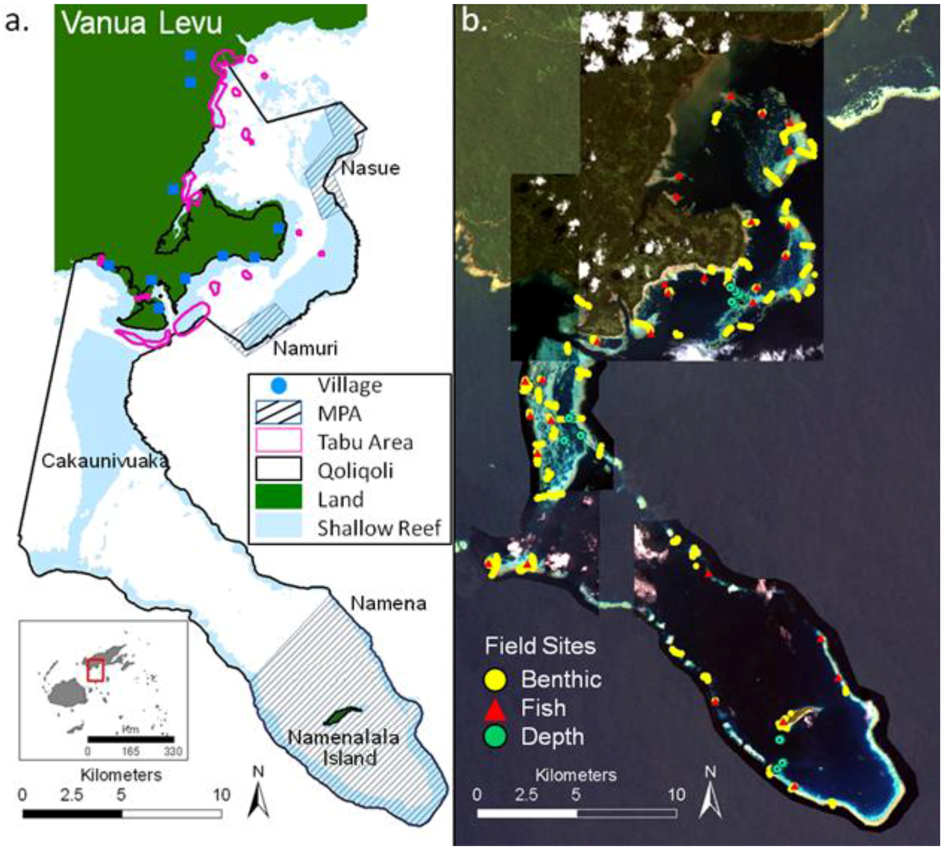
2. Study Area
3. Methods
3.1. Field Data Collection and Processing
3.1.1. Benthic Field Data

| First Level | Description | Second Level | Description |
|---|---|---|---|
| Coral (C) | >10% coral cover | Hard coral dominant | >70% Coral |
| Hard coral and Macroalgae | >10% Macroalgae | ||
| Hard coral and seagrass | >10% Seagrass | ||
| Hard coral and sand | >10% Sand | ||
| Hard coral and rubble | >10% Rubble | ||
| Hard coral and reef matrix | >10% Reef Matrix | ||
| Hard coral and less soft coral | >10% Soft Coral | ||
| Hard coral live and dead | >10% Dead Coral | ||
| Soft Coral (SC) | >10% soft coral cover | Soft coral dominant | >70% Soft Coral |
| Soft coral and macroalgae | >10% Macroalgae | ||
| Soft coral and seagrass | >10% Seagrass | ||
| Soft coral and sand | >10% Sand | ||
| Soft coral and rubble | >10% Rubble | ||
| Soft coral and reef matrix | >10% Reef Matrix | ||
| Soft coral and less hard coral | >10% Hard Coral | ||
| Macroalgae (MA) | <10% live coral cover, macroalgal cover >10% and dominant over seagrass | Macroalgae dominant | >70% Macroalgae |
| Macroalgae and Seagrass | >10% Seagrass | ||
| Macroalgae and Sand | >10% Sand | ||
| Macroalgae and Rubble | >10% Rubble | ||
| Macroalgae and Reef Matrix | >10% Reef Matrix | ||
| Macroalgae and dead coral | >10% dead Coral | ||
| Seagrass (SG) | <10% live coral cover, seagrass cover >10% and dominant over macroalgae | Seagrass dominant | >70% Seagrass |
| Seagrass and sand | >10% Sand | ||
| Seagrass and rubble | >10% Rubble | ||
| Non-Living Substratum (BS) | <10% live coral cover, <10% algal cover, <10% seagrass cover, >70% bare substratum | Sand dominant | >70% Sand |
| Rubble dominant | >70% Rubble | ||
| Reef matrix dominant | >70% Reef Matrix | ||
| Mud/silt dominant | >70% Mud/Silt | ||
| Sand/rubble dominant | >70% Sand/Rubble | ||
| Dead coral dominant | >70% Dead Coral |
3.1.2. Fish Field Data
3.2. Satellite Data
| Attribute | Quickbird | Ikonos | Landsat 5 TM |
|---|---|---|---|
| Data provider | Digitalglobe | Geoeye | NASA |
| Spatial resolution | 2.4 m | 4 m | 30 m |
| Maximum extent | 12 km × 12 km | 12 km × 12 km | 185 km × 185 km |
| Number of scenes | 3 | 2 | 1 |
| Acquisition year | 2006 | 2007 | 2002 |
| Mapping approach | Object based analysis | Object based analysis | Manual delineation |
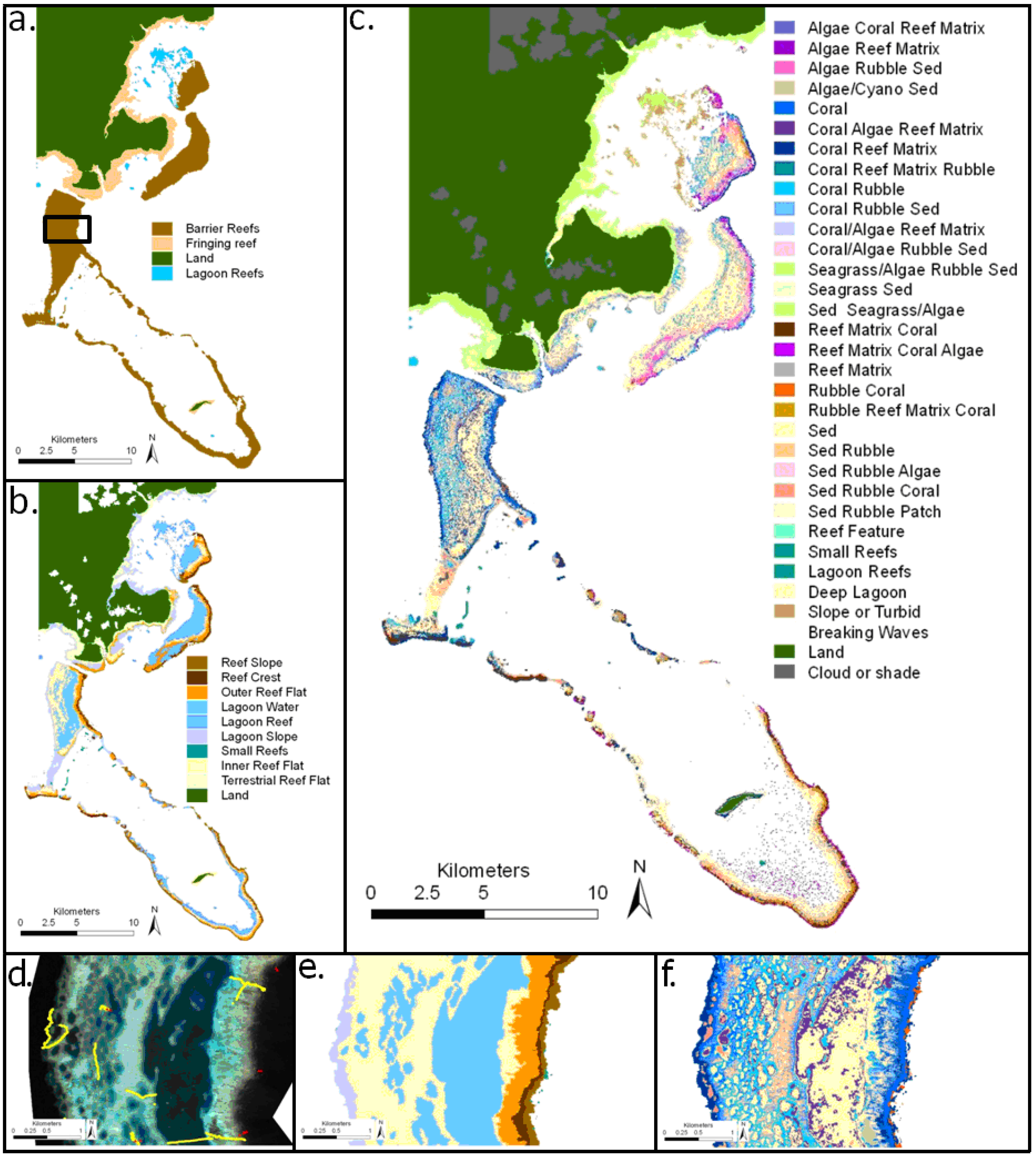
3.2.1. Object-Based Classification of Benthos and Geomorphic Zonation

3.2.2. Accuracy Assessment of Benthic and Geomorphic Maps
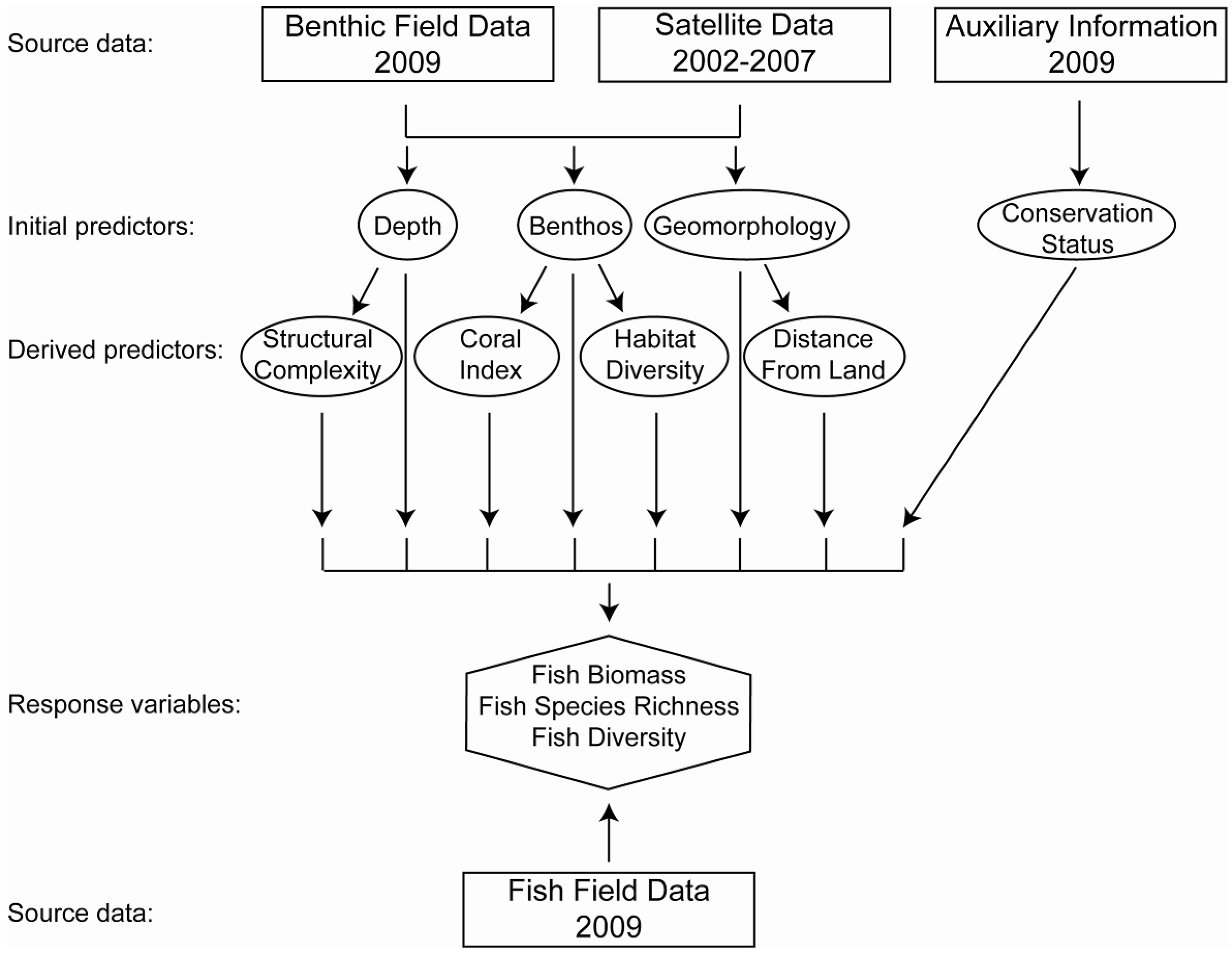
3.3. Mapping of Additional Variables
3.3.1. Depth
3.3.2. Structural Complexity
3.3.3. Live Coral Cover Index
3.3.4. Habitat Richness
3.3.5. Distance from Land
3.3.6. Conservation Status
3.4. Modeling Methods
4. Results
4.1. Geomorphic, Benthic and Depth Maps
4.2. Predictive Models
| Model type | Species richness | Biomass | Shannon diversity |
|---|---|---|---|
| Bagging | 6.395 | 613.6 | 0.563 |
| Boosted Regression Trees | 6.713 | 654.9 | 0.573 |
| Generalized Additive Model | 7.283 | 703.8 | 0.572 |
| Linear Model | 7.545 | 689.5 | 0.568 |
| Random Forest | 6.371 | 601.2 | 0.558 |
| Support Vector Machine | 7.434 | 637.8 | 0.558 |
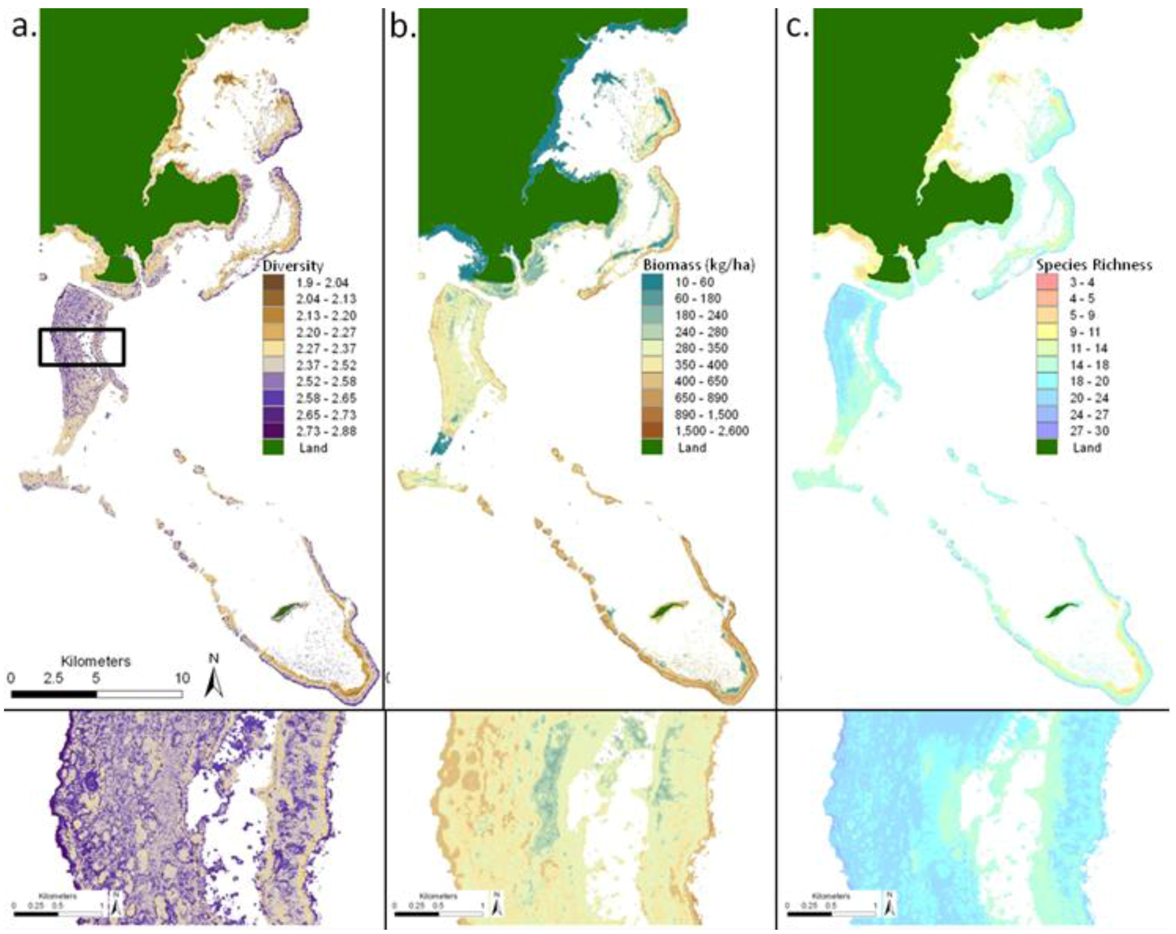
4.3. Predictive Maps
| Linear model | Generalized additive model | Bagging | Random forest | Boosted regression trees | Support vector machine | ||||||
|---|---|---|---|---|---|---|---|---|---|---|---|
| Species richness (ΔRMSE) | |||||||||||
| Cor 4 | 1.791 | Benthos | 1.801 | Benthos | 1.424 | Geo | 0.656 | Geo | 0.639 | Depth | 0.772 |
| Benthos | 1.374 | Cor 4 | 1.678 | Cor 500 | 0.178 | Depth | 0.183 | Benthos | 0.183 | Cur 4 | 0.173 |
| Geo | 1.215 | Geo | 1.239 | Depth | 0.127 | Benthos | 0.135 | Depth | 0.155 | A Cur 4 | 0.132 |
| Biomass (ΔRMSE) | |||||||||||
| Cor 4 | 139.4 | Cor 4 | 98.8 | Geo | 46.6 | Geo | 44.3 | Geo | 44.2 | Depth | 67.1 |
| Benthos | 112.8 | Benthos | 94.7 | Cor 1000 | 22.3 | Dist | 25.2 | Dist | 39.0 | Dist | 45.2 |
| Dist | 42.1 | Geo | 32.6 | Dist | 17.0 | Depth | 15.1 | Cur 300 | 24.0 | A Cur 4 | 10.3 |
| Shannon diversity (ΔRMSE × 10−3) | |||||||||||
| Geo | 16.9 | Geo | 23.1 | Geo | 12.4 | Benthos | 8.46 | Geo | 10.3 | Depth | 6.55 |
| Cor 200 | 10.7 | Cor 1000 | 4.38 | Benthos | 10.7 | Geo | 7.38 | Benthos | 5.99 | Cur 4 | 3.22 |
| Cor 30 | 7.89 | Dist | 0.92 | A Cur 10 | 5.39 | Cor 500 | 5.64 | Depth | 4.20 | A Cur 4 | 1.73 |
5. Discussion
6. Conclusion
Acknowledgements
References
- Bryant, D.; Burke, L.; McManus, J.; Spalding, M. Reefs at Risk: A Map-Based Indicator of Potential Threats to the World’s Coral Reefs; World Resources Institute: Washington, DC, USA, 1998; p. 56. [Google Scholar]
- Andrew, N.L.; Bene, C.; Hall, S.J.; Allison, E.H.; Heck, S.; Ratner, B.D. Diagnosis and management of small-scale fisheries in developing countries. Fish Fish. 2007, 8, 227–240. [Google Scholar] [CrossRef]
- Gaichas, S.K. A context for ecosystem-based fishery management: Developing concepts of ecosystems and sustainability. Marine Policy 2008, 32, 393–401. [Google Scholar] [CrossRef]
- Ainsworth, C.H.; Varkey, D.A.; Pitcher, T.J. Ecosystem simulations supporting ecosystem-based fisheries management in the Coral Triangle, Indonesia. Ecol. Model. 2008, 214, 361–374. [Google Scholar] [CrossRef]
- Lester, S.E.; Halpern, B.S.; Grorud-Colvert, K.; Lubchenco, J.; Ruttenberg, B.I.; Gaines, S.D.; Airame, S.; Warner, R.R. Biological effects within no-take marine reserves: A global synthesis. Marine Ecol. Progr. Ser. 2009, 384, 33–46. [Google Scholar] [CrossRef]
- Jupiter, S.D.; Egli, D.P. Ecosystem-based management in Fiji: Successes and challenges after five years of implementation. J. Marine Biology 2011. [Google Scholar] [CrossRef]
- Syms, C.; Jones, G.P. Disturbance, habitat structure, and the dynamics of a coral-reef fish community. Ecology 2000, 81, 2714–2729. [Google Scholar] [CrossRef]
- Gratwicke, B.; Speight, M.R. The relationship between fish species richness, abundance and habitat complexity in a range of shallow tropical marine habitats. J. Fish Biol. 2005, 66, 650–667. [Google Scholar] [CrossRef]
- Friedlander, A.M.; Parrish, J.D. Habitat characteristics affecting fish assemblages on a Hawaiian coral reef. J. Exp. Mar. Biol. Ecol. 1998, 224, 1–30. [Google Scholar] [CrossRef]
- Lara, E.N.; González, E.A. The relationship between reef fish community structure and environmental variables in the southern Mexican Caribbean. J. Fish Biol. 1998, 53, 209–221. [Google Scholar] [CrossRef]
- Connell, J.H. Diversity in tropical rain forests and coral reefs—High diversity of trees and corals is maintained only in a non-equilibrium state. Science 1978, 199, 1302–1310. [Google Scholar] [CrossRef] [PubMed]
- Jones, G.P.; McCormick, M.I.; Srinivasan, M.; Eagle, J.V. Coral decline threatens fish biodiversity in marine reserves. Proc. Nat. Acad. Sci. USA 2004, 101, 8251–8253. [Google Scholar] [CrossRef] [PubMed]
- Christensen, J.D.; Jeffrey, C.F.; Caldow, C.; Monaco, M.E.; Kendall, M.S.; Appeldoorn, R.S. Cross shelf habitat utilization patterns of reef fishes in southwestern Puerto Rico. Gulf Caribbean Res. 2003, 14, 9–27. [Google Scholar] [CrossRef]
- Dorenbosch, M.; Grol, M.G.G.; Christianen, M.J.A.; Nagelkerken, I.; van der Velde, G. Indo-Pacific seagrass beds and mangroves contribute to fish density coral and diversity on adjacent reefs. Marine Ecol. Progr. Ser. 2005, 302, 63–76. [Google Scholar] [CrossRef] [Green Version]
- Mumby, P.J.; Edwards, A.J.; Arias-Gonzalez, J.E.; Lindeman, K.C.; Blackwell, P.G.; Gall, A.; Gorczynska, M.I.; Harborne, A.R.; Pescod, C.L.; Renken, H.; Wabnitz, C.C.C.; Llewellyn, G. Mangroves enhance the biomass of coral reef fish communities in the Caribbean. Nature 2004, 427, 533–536. [Google Scholar] [CrossRef] [PubMed]
- Pittman, S.J.; McAlpine, C.A.; Pittman, K.M. Linking fish and prawns to their environment: a hierarchical landscape approach. Marine Ecol. Progr. Ser. 2004, 283, 233–254. [Google Scholar] [CrossRef]
- Pittman, S.J.; Christensen, J.D.; Caldow, C.; Menza, C.; Monaco, M.E. Predictive mapping of fish species richness across shallow-water seascapes in the Caribbean. Ecol. Model. 2007, 204, 9–21. [Google Scholar] [CrossRef]
- Grober-Dunsmore, R.; Frazer, T.K.; Beets, J.P.; Lindberg, W.J.; Zwick, P.; Funicelli, N.A. Influence of landscape structure, on reef fish assemblages. Landscape Ecol. 2008, 23, 37–53. [Google Scholar] [CrossRef]
- Mumby, P.J.; Green, E.P.; Edwards, A.J.; Clark, C.D. Coral reef habitat-mapping: How much detail can remote sensing provide? Marine Biol. 1997, 130, 193–202. [Google Scholar] [CrossRef]
- Mumby, P.J.; Hedley, J.D.; Chisholm, J.R.M.; Clark, C.D.; Ripley, H.; Jaubert, J. The cover of living and dead corals from airborne remote sensing. Coral Reefs 2004, 23, 171–183. [Google Scholar] [CrossRef]
- Newman, C.; Knudby, A.; LeDrew, E. Assessing the effect of management zonation on live coral cover using multi-date IKONOS satellite imagery. J. Appl. Remote Sens. 2007, 1. [Google Scholar] [CrossRef]
- Isoun, E.; Fletcher, C.; Frazer, N.; Gradie, J. Multi-spectral mapping of reef bathymetry and coral cover; Kailua Bay, Hawaii. Coral Reefs 2003, 22, 68–82. [Google Scholar]
- Lyzenga, D.R. Passive remote-sensing techniques for mapping water depth and bottom features. Appl. Opt. 1978, 17, 379–383. [Google Scholar] [CrossRef] [PubMed]
- Maritorena, S.; Morel, A.; Gentili, B. Diffuse-reflectance of oceanic shallow waters—Influence of water depth and bottom albedo. Limnol. Oceanogr. 1994, 39, 1689–1703. [Google Scholar] [CrossRef]
- Stumpf, R.P.; Holderied, K.; Sinclair, M. Determination of water depth with high-resolution satellite imagery over variable bottom types. Limnol. Oceanogr. 2003, 48, 547–556. [Google Scholar] [CrossRef]
- Roelfsema, C.; Phinn, S.; Jupiter, S.; Comley, M.; Beger, M.; Peterson, E. Object Based Analysis of High Spatial Resolution Imagery for Mapping Large Coral Reef Systems in The West Pacific at Geomorphic and Benthic Community Scales. In Proceedings of 2010 IEEE International Geoscience and Remote Sensing Symposium, Honolulu, HI, USA, 25–30 July 2010.
- Mellin, C.; Bradshaw, C.J.A.; Meekan, M.G.; Caley, M.J. Environmental and spatial predictors of species richness and abundance in coral reef fishes. Glob. Ecol. Biogeogr. 2010, 19, 212–222. [Google Scholar] [CrossRef]
- Knudby, A.; LeDrew, E.; Brenning, A. Predictive mapping of reef fish species richness, diversity and biomass in Zanzibar using IKONOS imagery and machine-learning techniques. Remote Sens. Environ. 2010, 114, 1230–1241. [Google Scholar] [CrossRef]
- Wedding, L.M.; Friedlander, A.M. Determining the Influence of Seascape Structure on Coral Reef Fishes in Hawaii Using a Geospatial Approach. Marine Geodesy 2008, 31, 246–266. [Google Scholar] [CrossRef]
- Pittman, S.J.; Costa, M.B.; Battista, T.A. Using lidar bathymetry and boosted regression trees to predict the diversity and abundance of fish and corals. J. Coastal Res. 2009, S1, 27–38. [Google Scholar] [CrossRef]
- Kuffner, I.B.; Brock, J.C.; Grober-Dunsmore, R.; Bonito, V.E.; Hickey, T.D.; Wright, C.W. Relationships between reef fish communities and remotely sensed rugosity measurements in Biscayne National Park, Florida, USA. Environ. Biol. Fish. 2007, 78, 71–82. [Google Scholar] [CrossRef]
- Mellin, C.; Andréfouët, S.; Ponton, D. Spatial predictability of juvenile fish species richness and abundance in a coral reef environment. Coral Reefs 2007, 26, 895–907. [Google Scholar] [CrossRef]
- Clarke, P.; Jupiter, S.D. Law, custom and community-based natural resource management in Kubulau District (Fiji). Environ. Conserv. 2010, 37, 98–106. [Google Scholar] [CrossRef]
- Cakacaka, A.; Jupiter, S.D.; Egli, D.P.; Moy, W. Status of Fin Fisheries in a Fijian Traditional Fishing Ground, Kubulau District, Vanua Levu; Technical Report No. 06/10; Wildlife Conservation Society: Suva, Fiji, 2010; p. 21. [Google Scholar]
- WCS. Ecosystem-Based Management Plan: Kubulau District, Vanua Levu, Fiji; Wildlife Conservation Society: Suva, Fiji, 2009; p. 121. [Google Scholar]
- Adams, V.M.; Mills, M.; Jupiter, S.D.; Pressey, R.L. Improving social acceptability of marine protected area networks: A method for estimating opportunity costs to multiple gear types in both fished and currently unfished areas. Biol. Conserv. 2010, 144, 350–361. [Google Scholar] [CrossRef]
- Roelfsema, C.; Phinn, S. Integrating field data with high spatial resolution multispectral satellite imagery for calibration and validation of coral reef benthic community maps. J. Appl. Remote Sens. 2010, 4, 043527. [Google Scholar] [CrossRef] [Green Version]
- Andréfouët, S.; Guzman, H.M. Coral reef distribution, status and geomorphology-biodiversity relationship in Kuna Yala (San Blas) archipelago, Caribbean Panama. Coral Reefs 2005, 24, 31–42. [Google Scholar] [CrossRef]
- Kohler, K.E.; Gill, S.M. Coral Point Count with Excel extensions (CPCe): A Visual Basic program for the determination of coral and substrate coverage using random point count methodology. Computer. Geosci. 2006, 32, 1259–1269. [Google Scholar] [CrossRef]
- English, S.; Wilkinson, C.; Baker, V. Survey Manual for Tropical Marine Resources; Australian Institute of Marine Science: Townsville, QLD, Australia, 1997; p. 390. [Google Scholar]
- Mumby, P.J.; Harborne, A.R. Development of a systematic classification scheme of marine habitats to facilitate regional management and mapping of Caribbean coral reefs. Biol. Conserv. 1999, 88, 155–163. [Google Scholar] [CrossRef]
- Hill, J.; Wilkinson, C. Methods for Ecological Monitoring of Coral Reefs. Version 1: A Resource for Managers; Australian Institute of Marine Science and Reef Check: Townsville, QLD, Australia, 2004; p. 117. [Google Scholar]
- Froese, R.; Pauly, D. Fishbase. Available online: www.fishbase.org. (accessed on 12 January 2009).
- Shannon, C.E.; Weaver, W. The Mathematical Theory of Communication; University of Illinois Press: Urbana, IL, USA, 1963; p. 144. [Google Scholar]
- Blaschke, T. Object based image analysis for remote sensing. ISPRS J. Photogramm. Remote Sens. 2010, 65, 2–16. [Google Scholar] [CrossRef]
- Phinn, S.; Roelfsema, C.; Mumby, P. Multi-scale image segmentation for mapping coral reef geomorphic and benthic community zone. Int. J. Remote Sens. 2011, in press. [Google Scholar]
- Congalton, R.; Green, K. Assessing the Accuracy of Remotely Sensed Data: Principles and Practices; Lewis Publishers: Boca Raton, FL, USA, 1999; p. 137. [Google Scholar]
- Knudby, A.; Brenning, A.; LeDrew, E. New approaches to modelling fish-habitat relationship. Ecol. Model. 2010, 221, 503–511. [Google Scholar] [CrossRef]
- R Core Development Team. R: A Language and Environment for Statistical Computing; R Foundation for Statistical Computing: Vienna, Austria, 2008; Available online: http://www.R-project.org/ (accessed on 28 February 2011).
- Hastie, T.; Tibshirani, R.; Friedman, J.H. The Elements of Statistical Learning: Data Mining, Inference, and Prediction; Springer-Verlag: New York, NY, USA, 2001; p. 763. [Google Scholar]
- Murray, K.; Conner, M.M. Methods to quantify variable importance: Implications for the analysis of noisy ecological data. Ecology 2009, 90, 348–355. [Google Scholar] [PubMed]
- Strobl, C.; Boulesteix, A.-L.; Zeileis, A.; Hothorn, T. Bias in random forest variable importance measures: Illustrations, sources and a solution. BMC Bioinf. 2007, 8. [Google Scholar] [CrossRef]
- Strobl, C.; Boulesteix, A.L.; Kneib, T.; Augustin, T.; Zeileis, A. Conditional variable importance for random forests. BMC Bioinf. 2008, 9. [Google Scholar] [CrossRef] [PubMed]
- Hamel, M.A.; Andréfouët, S. Using very high resolution remote sensing for the management of coral reef fisheries: Review and perspectives. Mar. Pollut. Bull. 2010, 60, 1397–1405. [Google Scholar] [CrossRef] [PubMed]
- Andréfouët, S.; Kramer, P.; Torres-Pulliza, D.; Joyce, K.E.; Hochberg, E.J.; Garza-Perez, R.; Mumby, P.J.; Riegl, B.; Yamano, H.; White, W.H.; Zubia, M.; Brock, J.C.; Phinn, S.R.; Naseer, A.; Hatcher, B.G.; Muller-Karger, F.E. Multi-site evaluation of IKONOS data for classification of tropical coral reef environments. Remote Sens. Environ. 2003, 88, 128–143. [Google Scholar] [CrossRef]
- Mumby, P.J.; Edwards, A.J. Mapping marine environments with IKONOS imagery: Enhanced spatial resolution can deliver greater thematic accuracy. Remote Sens. Environ. 2002, 82, 248–257. [Google Scholar] [CrossRef]
- Su, H.B.; Liu, H.X.; Heyman, W.D. Automated derivation of bathymetric information from multi-spectral satellite imagery using a Non-Linear Inversion Model. Marine Geodesy 2008, 31, 281–298. [Google Scholar] [CrossRef]
- Muslim, A.M.; Foody, G.M. DEM and bathymetry estimation for mapping a tide-coordinated shoreline from fine spatial resolution satellite sensor imagery. Int. J. Remote Sens. 2008, 29, 4515–4536. [Google Scholar] [CrossRef]
- Lyzenga, D.R.; Malinas, N.R.; Tanis, F.J. Multispectral bathymetry using a simple physically based algorithm. IEEE Trans. Geosci. Remote Sens. 2006, 44, 2251–2259. [Google Scholar] [CrossRef]
- Breiman, L. Random forests. Mach. Learn. 2001, 45, 5–32. [Google Scholar] [CrossRef]
- Grober-Dunsmore, R.; Frazer, T.K.; Lindberg, W.J.; Beets, J.P. Reef fish and habitat relationships in a Caribbean seascape: The importance of reef context. Coral Reefs 2007, 26, 201–216. [Google Scholar] [CrossRef]
- Friedlander, A.M.; Brown, E.K.; Monaco, M.E. Coupling ecology and GIS to evaluate efficacy of marine protected areas in Hawaii. Ecol. Appl. 2007, 17, 715–730. [Google Scholar] [CrossRef] [PubMed]
- Mumby, P.J. Beta and habitat diversity in marine systems: A new approach to measurement, scaling and interpretation. Oecologia 2001, 128, 274–280. [Google Scholar] [CrossRef]
- Turner, M.G.; Gardner, R.H.; O'Neill, R.V. Landscape Ecology in Theory and Practice: Pattern and Process; Springer Science + Business Media: New York, NY, USA, 2001; p. 404. [Google Scholar]
- Purkis, S.J.; Graham, N.A.J.; Riegl, B.M. Predictability of reef fish diversity and abundance using remote sensing data in Diego Garcia (Chagos Archipelago). Coral Reefs 2008, 27, 167–178. [Google Scholar] [CrossRef]
- Wedding, L.; Friedlander, A.M.; McGranaghan, M.; Yost, R.; Monaco, M. Using bathymetric LIDAR to define nearshore benthic habitat complexity: Implications for management of reef fish assemblages in Hawaii. Remote Sens. Environ. 2008, 112, 4159–4165. [Google Scholar] [CrossRef]
- Andréfouët, S.; Muller-Krager, F.E.; Robinson, J.A. Millennium Coral Reef Landsat Archive. Available online: http://oceancolor.gsfc.nasa.gov/cgi/landsat.pl (accessed on 13 October 2010).
- Andréfouët, S.; Muller-Krager, F.E.; Robinson, J.A.; Kranenburg, C.J.; Torres-Pulliza, D.; Spraggins, S.A.; Murch, B. Global Assessment of Modern Coral Reef Extent and Diversity for Regional Science and Management Applications: A View from Space. In Proceedings of 10th International Coral Reef Symposium, Okinawa, Japan, 28 June–2 July 2006; pp. 1732–1745.
- Andréfouët, S.; Gilbert, A.; Yan, L.; Remoissenet, G.; Payri, C.; Chancerelle, Y. The remarkable population size of the endangered clam Tridacna maxima assessed in Fangatau Atoll (Eastern Tuamotu, French Polynesia) using in situ and remote sensing data. Ices J. Mar. Sci. 2005, 62, 1037–1048. [Google Scholar]
- McClanahan, T.R.; Graham, N.A.J.; Maina, J.; Chabanet, P.; Bruggemann, J.H.; Polunin, N.V.C. Influence of instantaneous variation on estimates of coral reef fish populations and communities. Marine Ecol. Progr. Ser. 2007, 340, 221–234. [Google Scholar] [CrossRef]
© 2011 by the authors; licensee MDPI, Basel, Switzerland. This article is an open access article distributed under the terms and conditions of the Creative Commons Attribution license (http://creativecommons.org/licenses/by/3.0/).
Share and Cite
Knudby, A.; Roelfsema, C.; Lyons, M.; Phinn, S.; Jupiter, S. Mapping Fish Community Variables by Integrating Field and Satellite Data, Object-Based Image Analysis and Modeling in a Traditional Fijian Fisheries Management Area. Remote Sens. 2011, 3, 460-483. https://0-doi-org.brum.beds.ac.uk/10.3390/rs3030460
Knudby A, Roelfsema C, Lyons M, Phinn S, Jupiter S. Mapping Fish Community Variables by Integrating Field and Satellite Data, Object-Based Image Analysis and Modeling in a Traditional Fijian Fisheries Management Area. Remote Sensing. 2011; 3(3):460-483. https://0-doi-org.brum.beds.ac.uk/10.3390/rs3030460
Chicago/Turabian StyleKnudby, Anders, Chris Roelfsema, Mitchell Lyons, Stuart Phinn, and Stacy Jupiter. 2011. "Mapping Fish Community Variables by Integrating Field and Satellite Data, Object-Based Image Analysis and Modeling in a Traditional Fijian Fisheries Management Area" Remote Sensing 3, no. 3: 460-483. https://0-doi-org.brum.beds.ac.uk/10.3390/rs3030460