Advantages of the Boresight Effect in Hyperspectral Data Analysis


Abstract
:1. Introduction
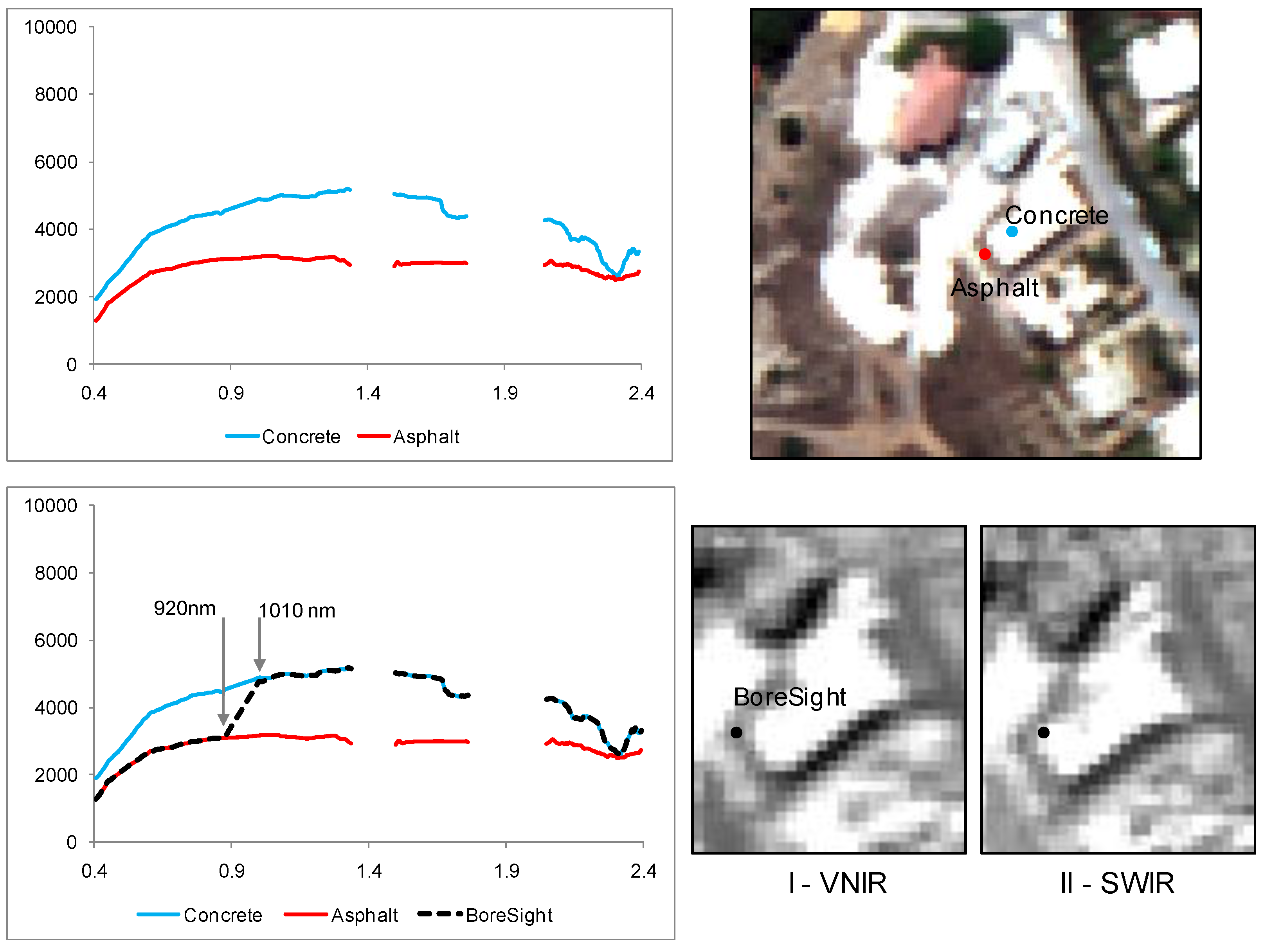
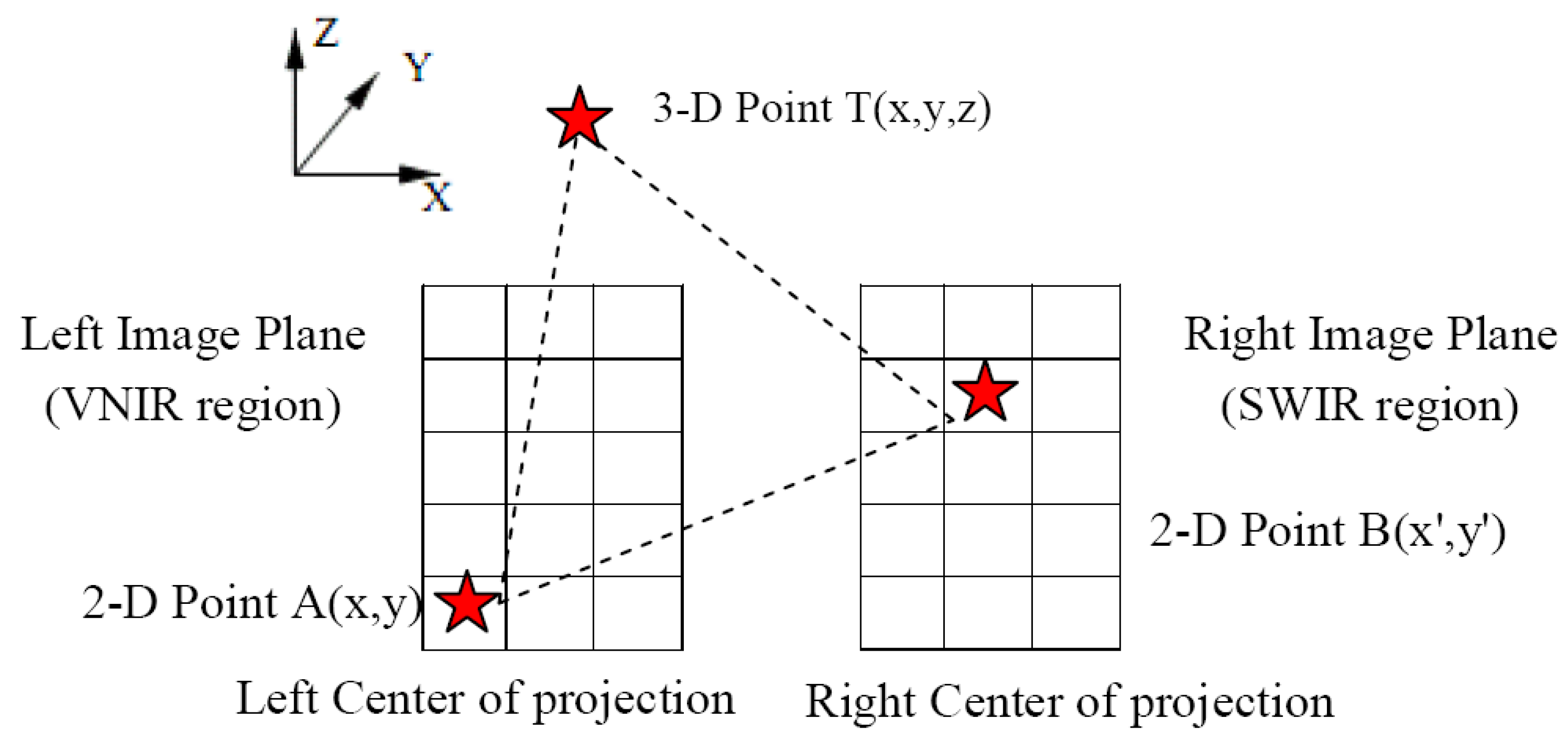
2. Boresight Effect in a Multisensor System


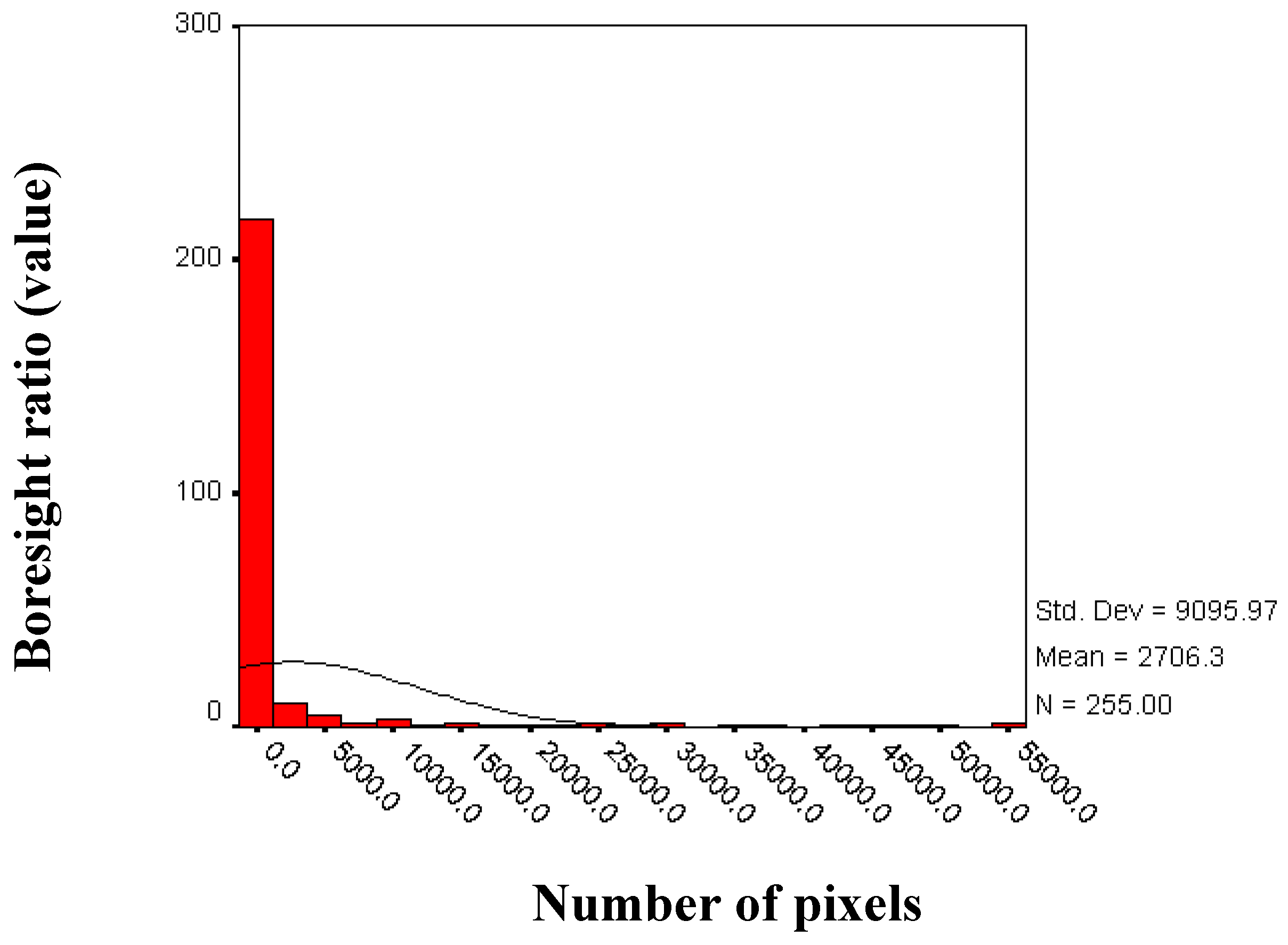
| N | Mean | Std. | Variance | Skewness | ||
|---|---|---|---|---|---|---|
| Statistic | Statistic | Std. Error | Statistic | Statistic | Statistic | Std. Error |
| 255 255 | 2,706.325 | 569.6115 | 9,095.966 | 8.3E + 07 | 4.132 | 0.153 |

3. Boresight Applications: Results and Discussion
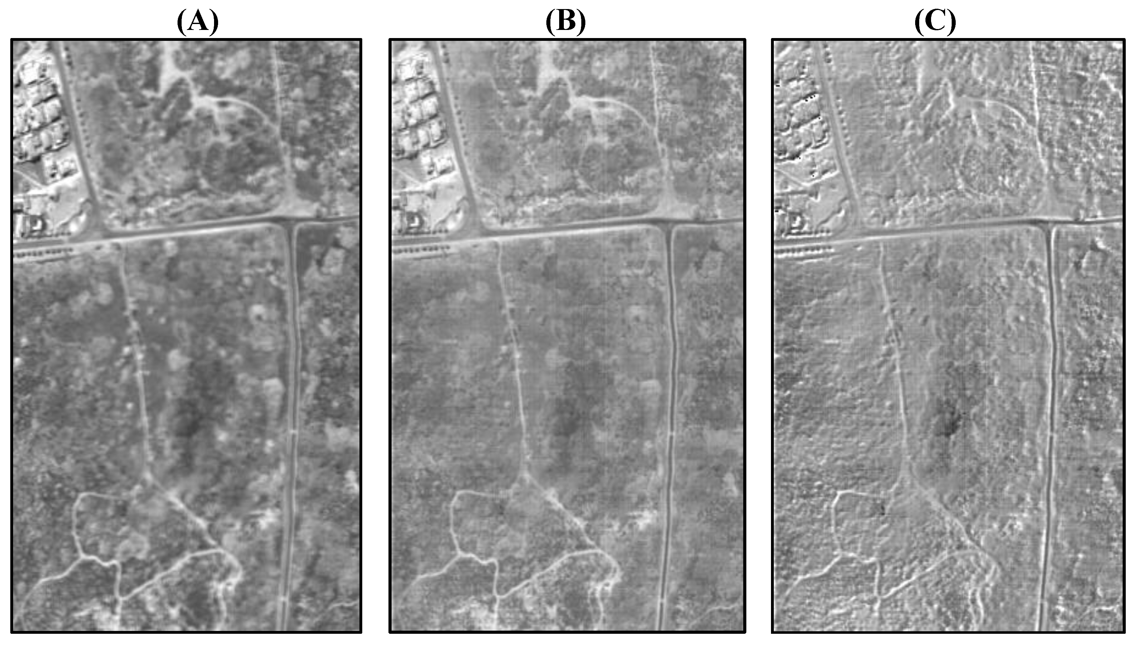
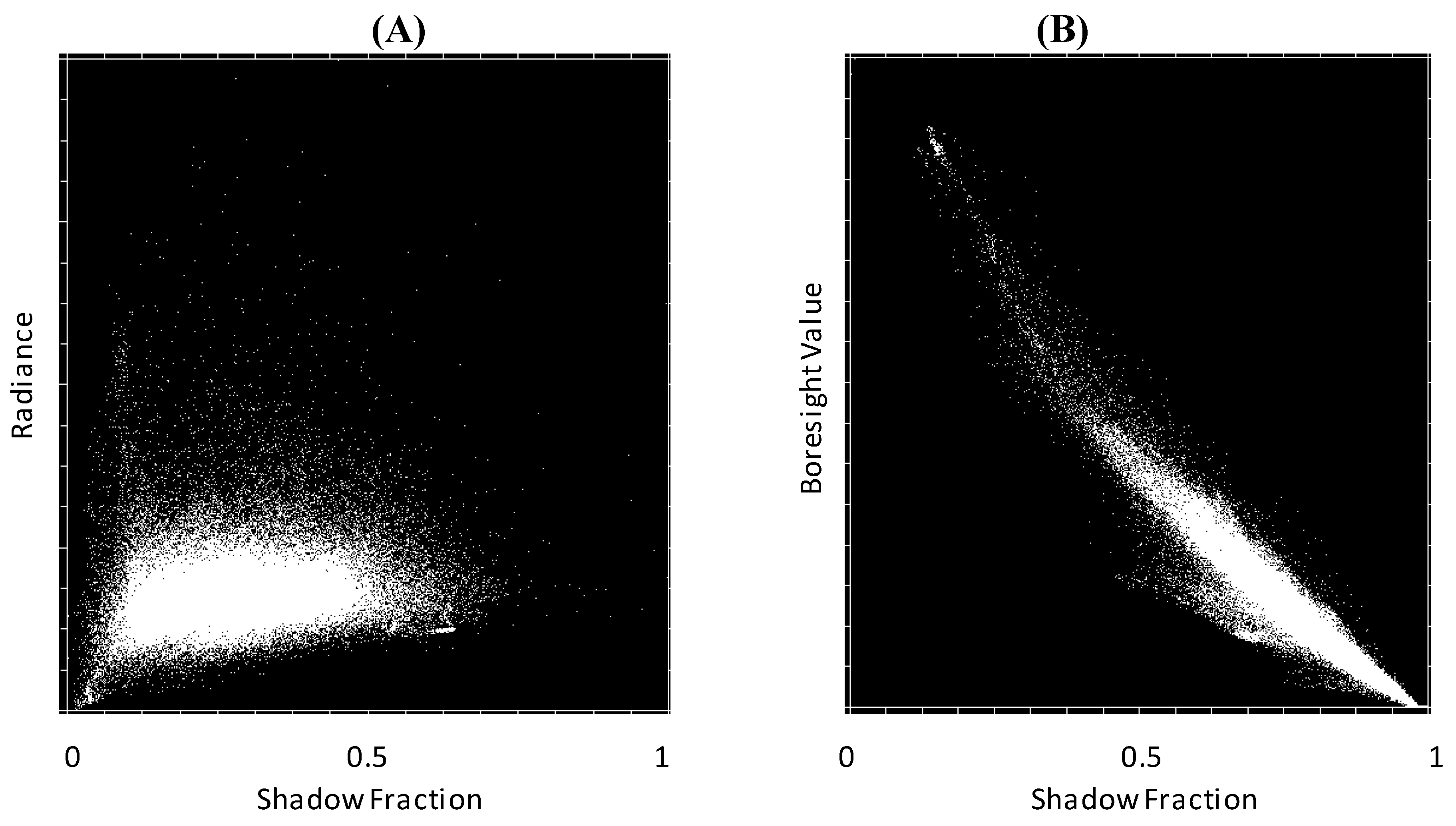
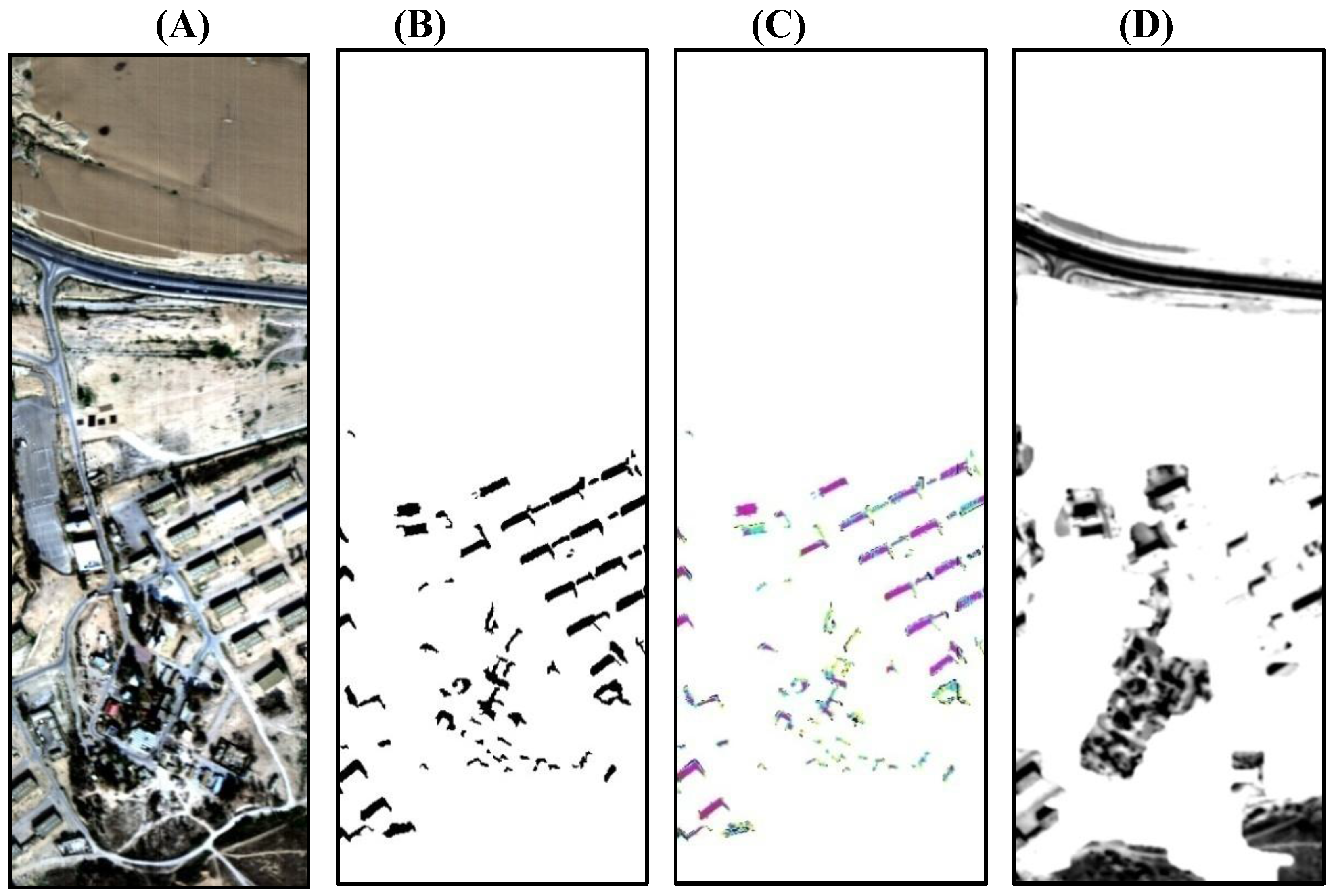
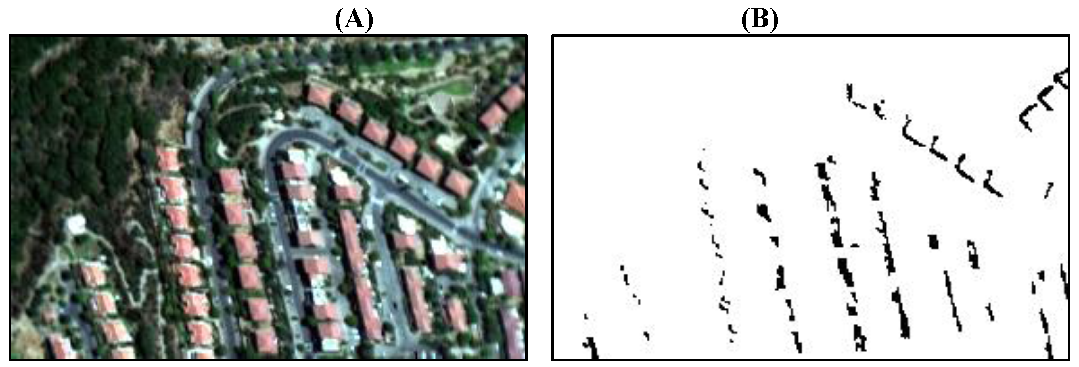
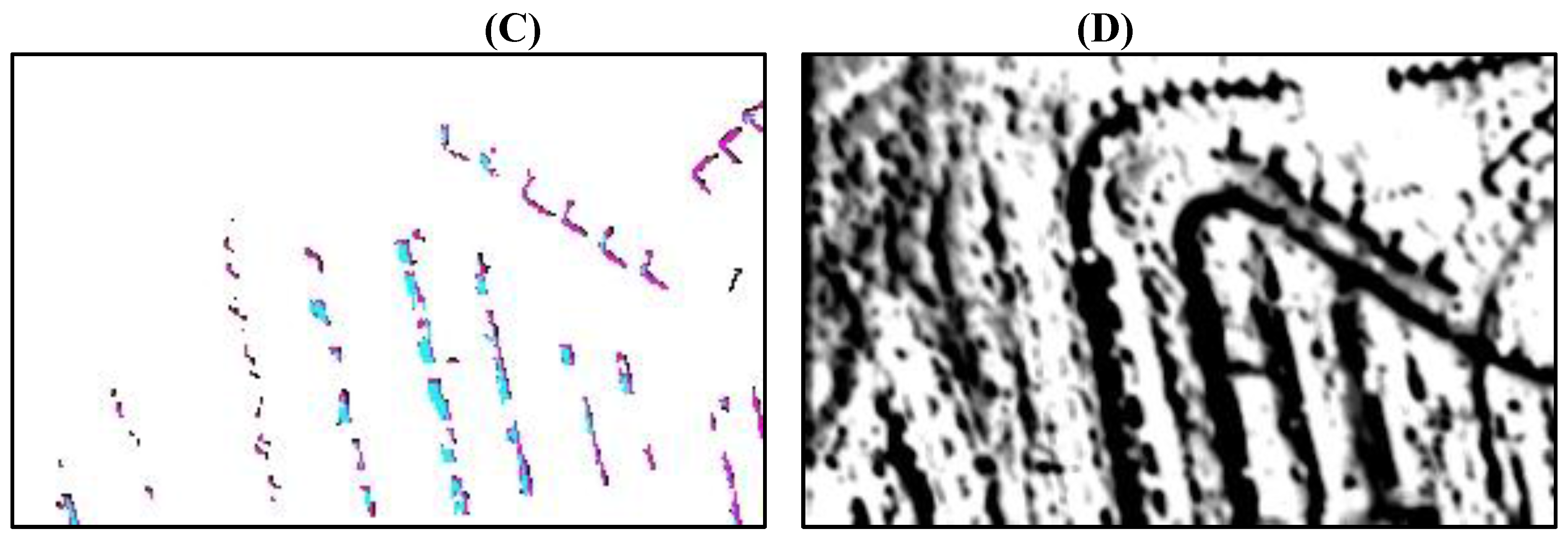
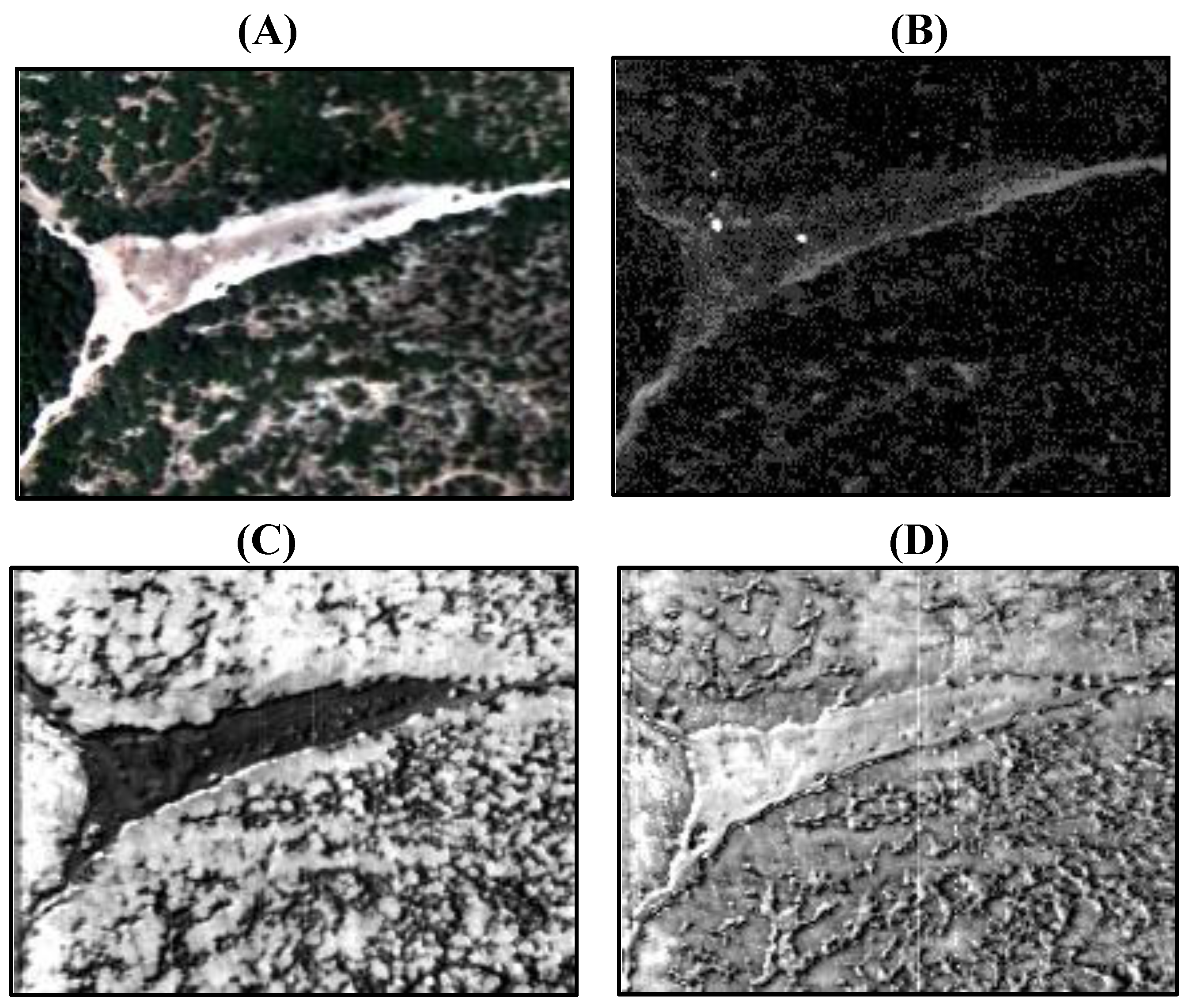
3.1. Enhancing the Shadow Effect


| Class ID | Boresight value (band ratio) | Shadow fraction (ground truth) |
|---|---|---|
| #1 (maroon) | 4–3.4 | 80–100% |
| #2 (magenta) | 3.4–2.5 | 50–80% |
| #3 (cyan) | 2.5–2.1 | 20–50% |
| #4 (yellow) | 2.1–1.9 | 10–20% |


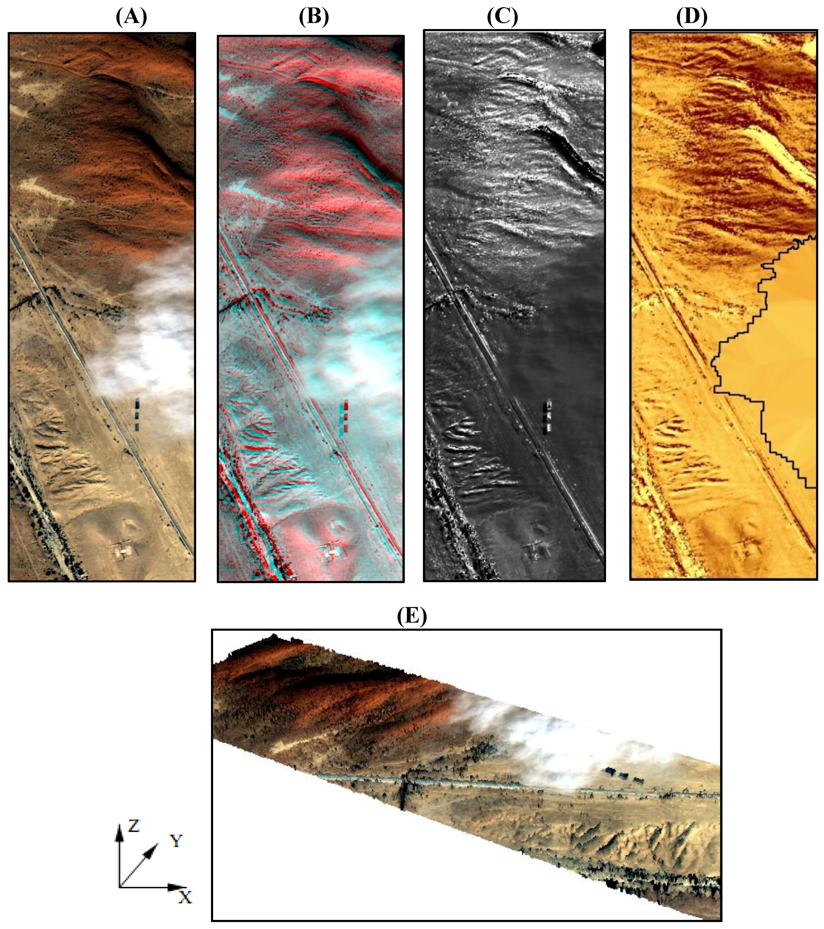
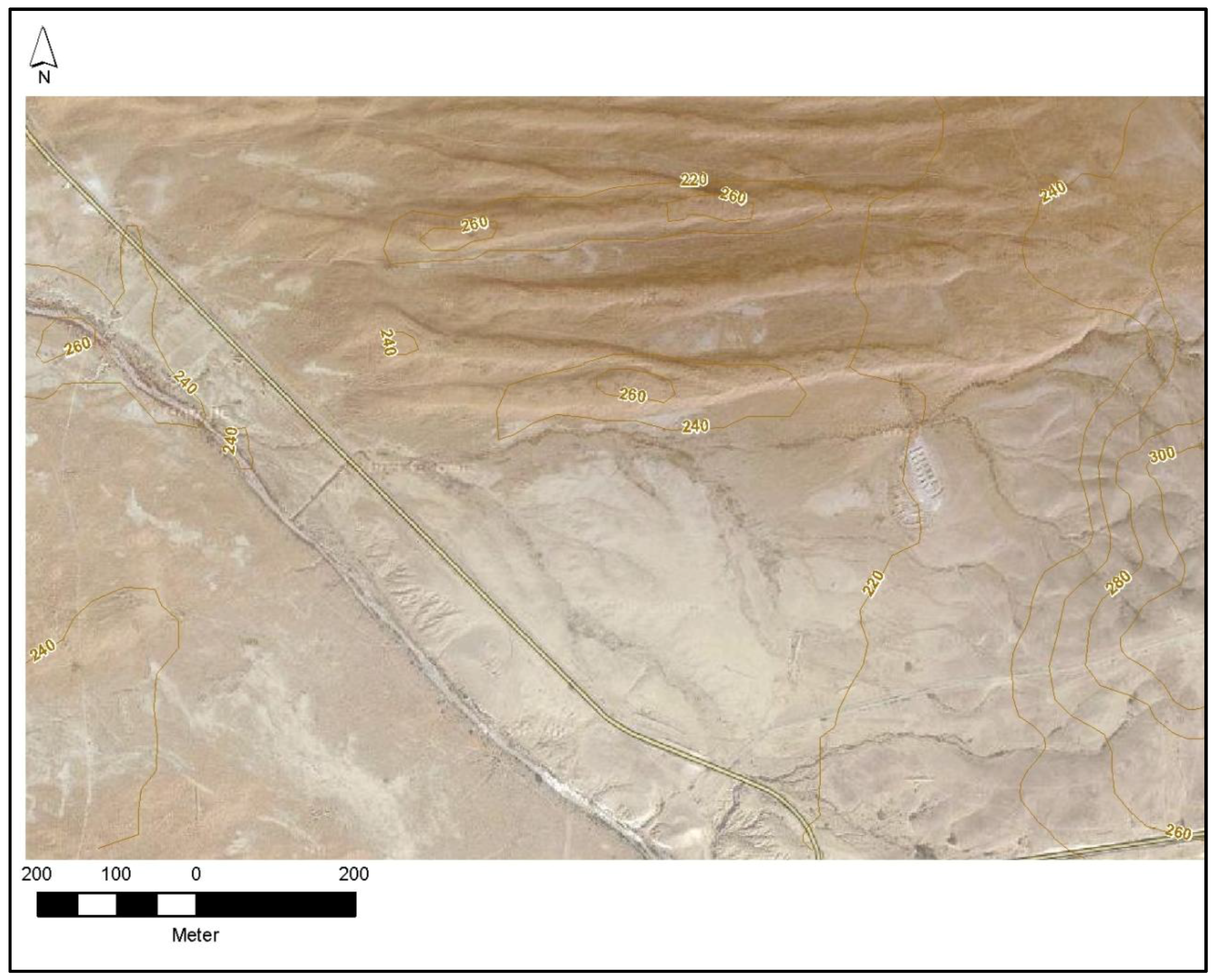
3.2. Stereo 3-D Map

 30 m), (E) AISA-Dual image in 3-D view (x axis 1,500 m, y axis 500 m, z axis (relative to the scene elevation) 30 m).
30 m), (E) AISA-Dual image in 3-D view (x axis 1,500 m, y axis 500 m, z axis (relative to the scene elevation) 30 m).
30 m), (E) AISA-Dual image in 3-D view (x axis 1,500 m, y axis 500 m, z axis (relative to the scene elevation) 30 m).

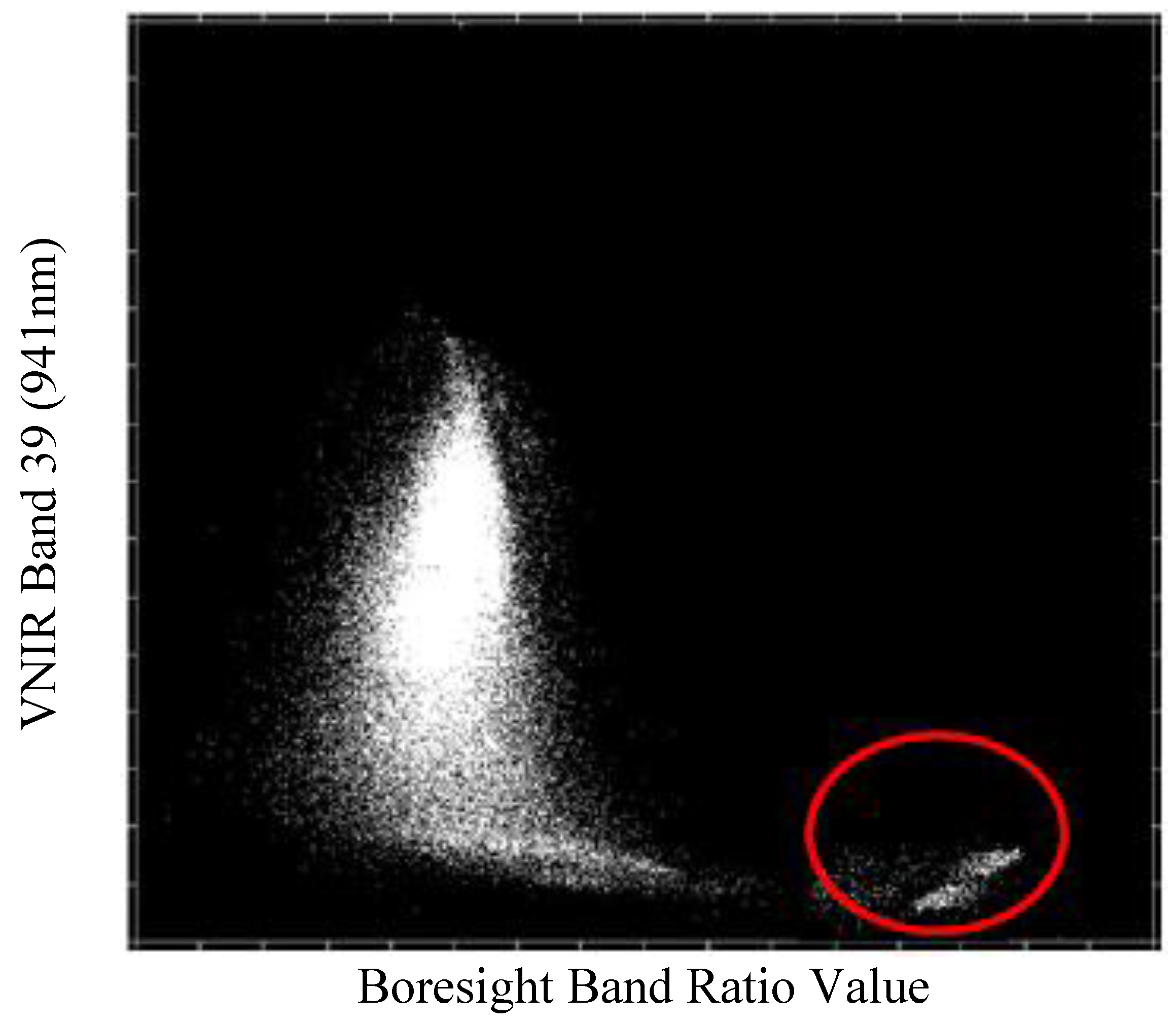
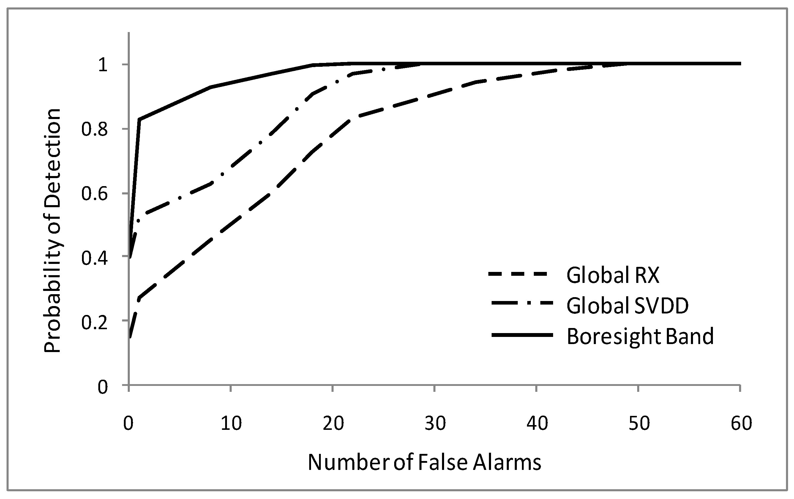
3.3. Unmixing and Anomaly Detection


4. Discussion
5. Conclusions
References and Notes
- Goetz, A.F.H.; Vane, G.; Solomon, J.; Rock, B.N. Imaging spectrometry for Earth remote sensing. Science 1985, 228, 1147–1153. [Google Scholar] [CrossRef] [PubMed]
- Boardman, J.W.; Kruse, F.A. Automated Spectral Analysis: A Geologic Example Using AVIRIS Data, North Grapevine Mountains, Nevada. In Proceedings of Tenth Thematic Conference on Geologic Remote Sensing, San Antonio, TX, USA, 9–12 May 1994; pp. I-407–I-418.
- Budkewitsch, P.; Peshko, M. The Maturing of Hyperspectral Imaging Technology and Its Benefits for Exploration Programs. In Proceeding of PDAC 2005 International Convention, Trade Show and Investors Exchange, Toronto, ON, Canada, 6–9 March 2005.
- Blackburn, G.A. Spectral indices for estimating photosynthetic pigment concentrations: A test using senescent tree leaves. Int. J. Remote Sens. 1998, 19, 657–675. [Google Scholar] [CrossRef]
- Cho, M.A.; Skidmore, A.K. A new technique for extracting the red edge position from hyperspectral data: the linear extrapolation method. Remote Sens. Environ. 2006, 101, 181–193. [Google Scholar] [CrossRef]
- Abuelgasim, A.A.; Ross, W.D.; Gopal, S. Change detection using Adaptive Fuzzy Neural Networks: Environmental damage assessment after the Gulf War. Remote Sens. Environ. 1999, 70, 208–223. [Google Scholar] [CrossRef]
- Coops, N.; Stanford, M.; Old, K.; Dudzinski, M.; Culvenor, D.; Stone, C. Assessment of dothistroma needle blight of pinus radiata using airborne hyperspectral imagery. Phytopathology 2003, 93, 1524–1532. [Google Scholar] [CrossRef] [PubMed]
- Thomas, C.D.; Cameron, A.; Green, R.E.; Bakkenes, M.; Beaumont, L.J.; Collingham, Y.C. Extinction risk from climate change. Nature 2004, 427, 145–148. [Google Scholar] [CrossRef] [PubMed] [Green Version]
- Clark, D.A.; Piper, S.C.; Keeling, C.D.; Clark, D.B. Tropical rain forest tree growth and atmospheric carbon dynamics linked to interannual temperature variation during 1984–2000. Proc. Natl. Acad. Sci. USA 2003, 10, 5852–5857. [Google Scholar] [CrossRef] [PubMed]
- Peterson, D.L.; Aber, J.D.; Matson, P.A.; Card, D.H.; Swanberg, N.; Wessman, C.; Spanner, M. Remote sensing of forest canopy and leaf biochemical contents. Remote Sens. Environ. 1988, 24, 85–108. [Google Scholar] [CrossRef]
- Chen, Z.; Elvidge, C.D.; Groeneveld, D.P. Monitoring seasonal dynamics of arid land vegetation using AVIRIS data. In Summaries of the 6th Annual JPL Airborne Earth Science Workshop, Proceedings of AVIRIS Workshop, Pasadena, CA, USA, 4–8 March 1996; JPL Pub. 96-4. Jet Propulsion Laboratory, California Institute of Technology: Pasadena, CA, USA, 1996; Volume 1, pp. 29–38. [Google Scholar]
- Richardson, L.L.; Ambrosia, V.G. Algal accessory pigment detection using AVIRIS image-derived spectral radiance data. In Summaries of the 6th Annual JPL Airborne Earth Science Workshop, Proceedings of AVIRIS Workshop, Pasadena, CA, USA, 4–8 March 1996; JPL Pub. 96-4. Jet Propulsion Laboratory, California Institute of Technology: Pasadena, CA, USA, 1996; Volume 1, pp. 189–196. [Google Scholar]
- Carder, K.L.; Reinersman, P.; Chen, R.F.; Muller-Karger, F.; Davis, C.O.; Hamilton, M.K. AVIRIS calibration and application in coastal oceanic environments. Remote Sens. Environ. 1993, 44, 205–216. [Google Scholar] [CrossRef]
- Acito, N.; Corsini, G.; Diani, M. Adaptive detection algorithm for full-pixel targets in hyperspectral images. IEE Proc. Vis. Image Signal Process. 2005, 152, 731–740. [Google Scholar] [CrossRef]
- Banerjee, A.; Burlina, P.; Diehl, C. A support vector method for anomaly detection in hyperspectral imagery. IEEE Trans. Geosci. Remote Sens. 2006, 44, 2282–2291. [Google Scholar] [CrossRef]
- Grejner-Brzezinska, D.A. Direct Exterior Orientation of Airborne Imagery with GPS/INS System: Performance Analysis. Navigation 1999, 46, 261–270. [Google Scholar] [CrossRef]
- Moffit, F.; Mikhail, E.M. Photogrammetry; Harper and Row: New York, NY, USA, 1980. [Google Scholar]
- Mostafa, M.M.R.; Schwarz, K.P. Digital image georeferencing from a multiple camera system by GPS/INS. ISPRS J. Photogramm. Remote Sens. 2001, 56, 1–12. [Google Scholar] [CrossRef]
- Chen, J.M. Optically-based methods for measuring seasonal variation of leaf area index in boreal conifer stands. Agr. Forest Meteorol. 1996, 80, 135–163. [Google Scholar] [CrossRef]
- Häme, T.; Salli, A.; Andersson, K.; Lohi, A. A new methodology for the estimation of biomass of conifer-dominated boreal forest using NOAA AVHRR data. Int. J. Remote Sens. 1997, 18, 3211–3243. [Google Scholar] [CrossRef]
- Nilson, T.; Anniste, J.; Lang, M.; Praks, J. Determination of needle area indices of forest canopies in the NOPEX region by ground-based optical measurements and satellite images. Agr. Forest Meteorol. 1999, 98, 449–462. [Google Scholar] [CrossRef]
- Eklundh, L.; Harrie, L.; Kuusk, A. Investigating relationships between Landsat ETM+ sensor data and leaf area index in boreal conifer forest. Remote Sens. Environ. 2001, 78, 239–251. [Google Scholar] [CrossRef]
- Rautiainen, M.; Stenberg, P.; Nilson, T.; Kuusk, A.; Smolander, H. Application of a forest reflectance model in estimating leaf area index of Scots pine stands using Landsat 7 ETM reflectance data. Can. J. Remote Sens. 2003, 29, 314–323. [Google Scholar] [CrossRef]
- Festinger, L. A statistical test for means of samples from skew population. Psychometrika 1943, 8, 205–210. [Google Scholar] [CrossRef]
- Pearson, K. Contributions to the mathematical theory of evolution, II: Skew variation in homogeneous material. Phil. Trans. Roy. Soc. London 1895, 186, 343–414. [Google Scholar] [CrossRef]
- Cochran, W.G. Sampling Techniques; Wiley: New York, NY, USA, 1977. [Google Scholar]
- Schläpfer, D.; Richter, R.; Hueni, A. Recent development in Operational Atmospheric and Radiometric Correction of Hyperspectral Imagery. In Proceedings of 6th EARSeL SIG IS Workshop, Tel-Aviv, Israel, 16–18 March 2009.
- Welch, W.J.; Yu, T.K.; Kang, S.M.; Sacks, J. Computer experiments for quality control by parameter design. J. Quality Technol. 1990, 22, 15–22. [Google Scholar]
- Boos, D.D.; Hughes-Oliver, J.M. How large does n have to be for Z and t intervals? Amer. Statist. 2000, 54, 121–128. [Google Scholar] [CrossRef]
- Pope, A.R. Learning to Recognize Objects in Images: Acquiring and Using Probabilistic Models of Appearance. Ph.D. Thesis, The University of British Columbia, Vancouver, BC, Canada, 1995. [Google Scholar]
- Press, W.H.; Flannery, B.P.; Teukolsky, S.A.; Vetterling, W.T. Numerical Recipes in C; Cambridge University Press: Cambridge, UK, 1988; pp. 681–688. [Google Scholar]
- Shashua, A. Trilinear Tensor: The Fundamental Construct of Multiple View Geometry and Its Applications; Institute of Computer Science, The Hebrew University: Jerusalem, Israel, 1997. [Google Scholar]
- Shashua, A.; Werman, M. Fundamental Tensor: On the Geometry of Three Perspective Views; Institute of Computer Science, The Hebrew University: Jerusalem, Israel, 1995. [Google Scholar]
- Torr, P.H.S.; Zisserman, A. Robust parametrization and computation of the tri-focal tensor. Image Vis. Comput. 1997, 15, 591–605. [Google Scholar] [CrossRef]
- Welch, G.; Bishop, G. An Introduction to the Kalman Filter; University of North Carolina: Chapel Hill, NC, USA, 1997. [Google Scholar]
- Toutin, T. Generating DEM from stereo-images with a photogrammetric approach: Examples with VIR and SAR data. EARSeL Adv. Remote Sens. 1995, 4, 110–117. [Google Scholar]
- Toutin, T. Three-dimensional topographic mapping with ASTER stereo data in rugged topography. IEEE Trans. Geosci. Remote Sens. 2002, 40, 2241–2247. [Google Scholar] [CrossRef]
- PCI Geomatics Group. OrthoEngineSE 3D, v7.0 Reference Manual; Version 7; PCI Geomatics Group: Richmond Hill, ON, Canada, 2001. [Google Scholar]
- Welch, W.J.; Buck, R.J.; Sacks, J.; Wynn, H.P.; Mitchell, T.J.; Morris, M.D. Screening, predicting, and computer experiments. Technometrics 1992, 34, 15–25. [Google Scholar] [CrossRef]
- Sacks, J.; Welch, W.J.; Mitchell, T.J.; Wynn, H.P. Design and analysis of computer experiments. Statist. Sci. 1989, 4, 409–435. [Google Scholar] [CrossRef]
- Reed, I.S.; Yu, X. Adaptivemultiple-band CFAR detection of an optical pattern with unknown spectral distribution. IEEE Trans. Acoust. Signal Process. 1990, 38, 1760–1770. [Google Scholar] [CrossRef]
- Yu, X.; Reed, I.S.; Stocker, A.D. Comparative performance analysis of adaptive multispectral detectors. IEEE Trans. Signal Process. 1993, 41, 2639–2656. [Google Scholar] [CrossRef]
- Yu, X.; Hoff, L.E.; Reed, I.S.; Chen, A.M.; Stotts, L.B. Automatic target detection and recognition in multispectral imagery: A unified ML detection and estimation approach. IEEE Trans. Image Process. 1997, 6, 143–156. [Google Scholar] [PubMed]
- Banerjee, A.; Burlina, P.; Meth, R. Fast Hyperspectral Anomaly Detection via SVDD. In Proceedings of 2007 IEEE International Conference on Image Processing, San Antonio, TX, USA, 16 September–19 October 2007.
- Banerjee, A.; Burlina, P.; Diehl, C. Support vector methods for anomaly detection in hyperspectral imagery. IEEE Trans. Geosci. Remote Sens. 2006, 44, 2282–2291. [Google Scholar] [CrossRef]
- Settle, J.J.; Drake, N.A. Linear mixing and the estimation of ground cover proportions. Int. J. Remote Sens. 1993, 14, 1159–1177. [Google Scholar] [CrossRef]
© 2011 by the authors; licensee MDPI, Basel, Switzerland. This article is an open access article distributed under the terms and conditions of the Creative Commons Attribution license (http://creativecommons.org/licenses/by/3.0/).
Share and Cite
Brook, A.; Ben-Dor, E. Advantages of the Boresight Effect in Hyperspectral Data Analysis. Remote Sens. 2011, 3, 484-502. https://0-doi-org.brum.beds.ac.uk/10.3390/rs3030484
Brook A, Ben-Dor E. Advantages of the Boresight Effect in Hyperspectral Data Analysis. Remote Sensing. 2011; 3(3):484-502. https://0-doi-org.brum.beds.ac.uk/10.3390/rs3030484
Chicago/Turabian StyleBrook, Anna, and Eyal Ben-Dor. 2011. "Advantages of the Boresight Effect in Hyperspectral Data Analysis" Remote Sensing 3, no. 3: 484-502. https://0-doi-org.brum.beds.ac.uk/10.3390/rs3030484