Design and Development of a Multi-Purpose Low-Cost Hyperspectral Imaging System

Abstract

Hyperspectral image analysis is gaining momentum in a wealth of natural resources and agricultural applications facilitated by the increased availability of low-cost imaging systems. In this study, we demonstrate the development of the Vegetation Mobile Mapping System (VMMS), a low-cost hyperspectral sensing system that is supported by consumer-grade digital camera(s). The system was developed using off-the-shelf imaging and navigation components mainly for ground-based applications. The system integrates a variety of components including timing and positioning GPS receivers and an Inertial Measurement Unit (IMU). The system was designed to be modular and interoperable allowing the imaging components to be used with different navigation systems. The technique used for synchronizing captured images with GPS time was presented. A relative radiometric calibration technique utilizing images of homogeneous targets to normalize pixel gain and offset parameters was used. An empirical spectral calibration method was used to assign wavelengths to image bands. Data acquisition parameters to achieve appropriate spatial coverage were presented. The system was tested in ground-based data collection and analysis experiments that included water quality and vegetation studies.

1. Introduction

Vegetation characterization using multispectral and hyperspectral images is a topic of significant research interest. Spectral responses of plants are analyzed and used in many applications such as classifying vegetation [1]. Hyperspectral imagery measures the spectral response at each pixel in a series of narrow and adjacent wavelength bands. This continuous representation of the spectrum at each pixel facilitates many types of analysis. Hyperspectral imagery has been used in many applications including assessing plant stress [2], identifying invasive species [3], estimating water quality parameters of both open oceans [4,5] and turbid inland waters [6], agricultural crop classification and yield estimation [7,8], and characterization of ecosystems [9,10].

Many hyperspectral imaging systems have been developed since NASA’s Airborne Visible InfraRed Imaging Spectrometer (AVIRIS) system [11,12] was introduced in the late 1980s. Some of these systems were airborne such as the Hyperspectral Mapper (HyMap) [13], the Compact Airborne Spectrographic Imager (CASI) [14], the Airborne Visible/Infrared Imaging Spectrometer AVIS [15], Airborne Imaging Spectrometer for Applications (AISA), and the Hyperspectral Digital Imagery Collection Experiment (HYDICE) [16]. Other hyperspectral systems were carried onboard satellite platforms such as the NASA’s Earth Observing-1 mission (EO-1) Hyperion system [17]. Although such systems have supplied the remote sensing community with valuable images, they lacked full implementation control due to cost and availability factors. Other limitations included relatively low spatial resolution and atmospheric effects due to large object-sensor proximity.

Portable handheld spectrometer devices provide spectral data that can be analyzed directly [18,19] or incorporated in the calibration and analysis process of other hyperspectral images [20,21]. Such devices have been used frequently in forestry and agricultural applications. They have rarely been utilized in mobile mapping applications. Data taken by handheld spectrometers is localized, limiting analysis to the spectral information captured by the device at certain location, and does not account for the spatial relationships between imaged objects. Recently, ground-based mobile sensors have been introduced in precision agriculture with sensors developed specifically to measure soil moisture content, plant stress, etc. Most of these systems utilize only a few bands in the spectrum and are limited to analyzing plant irrigation/fertilization needs [22,23], or identifying harmful weeds [24].

In the last few years, low-cost hyperspectral system development emerged motivated by application needs and facilitated by the availability of commercial Original Equipment Manufacturer (OEM) spectrographs and digital cameras capable of sensing in an extended range of the spectrum, especially in the visible/Near Infrared range. Many of the commercially available systems are stationary. They form images line-by-line by rotating the sensor or through a rotating mirror mounted in front of the lens [25,26]. Although this type of system can be used in many ground-based applications, its lack of mobility hinders wide scale implementation. In this research, we present a low-cost close-range mobile mapping system (Vegetation Mobile Mapping System VMMS) comprised of linear array hyperspectral sensor and consumer-grade multispectral camera(s) that can be mounted on multiple ground-based mobile platforms. The sensor is currently being used in several applications such as precision agriculture, water quality parameter estimation, and road right-of-way vegetation analysis. Although the main objective of this system is to study vegetation, its use as an educational tool in graduate courses was invaluable. Detailed information about system components, design, development, and calibration is presented.

2. System Configuration

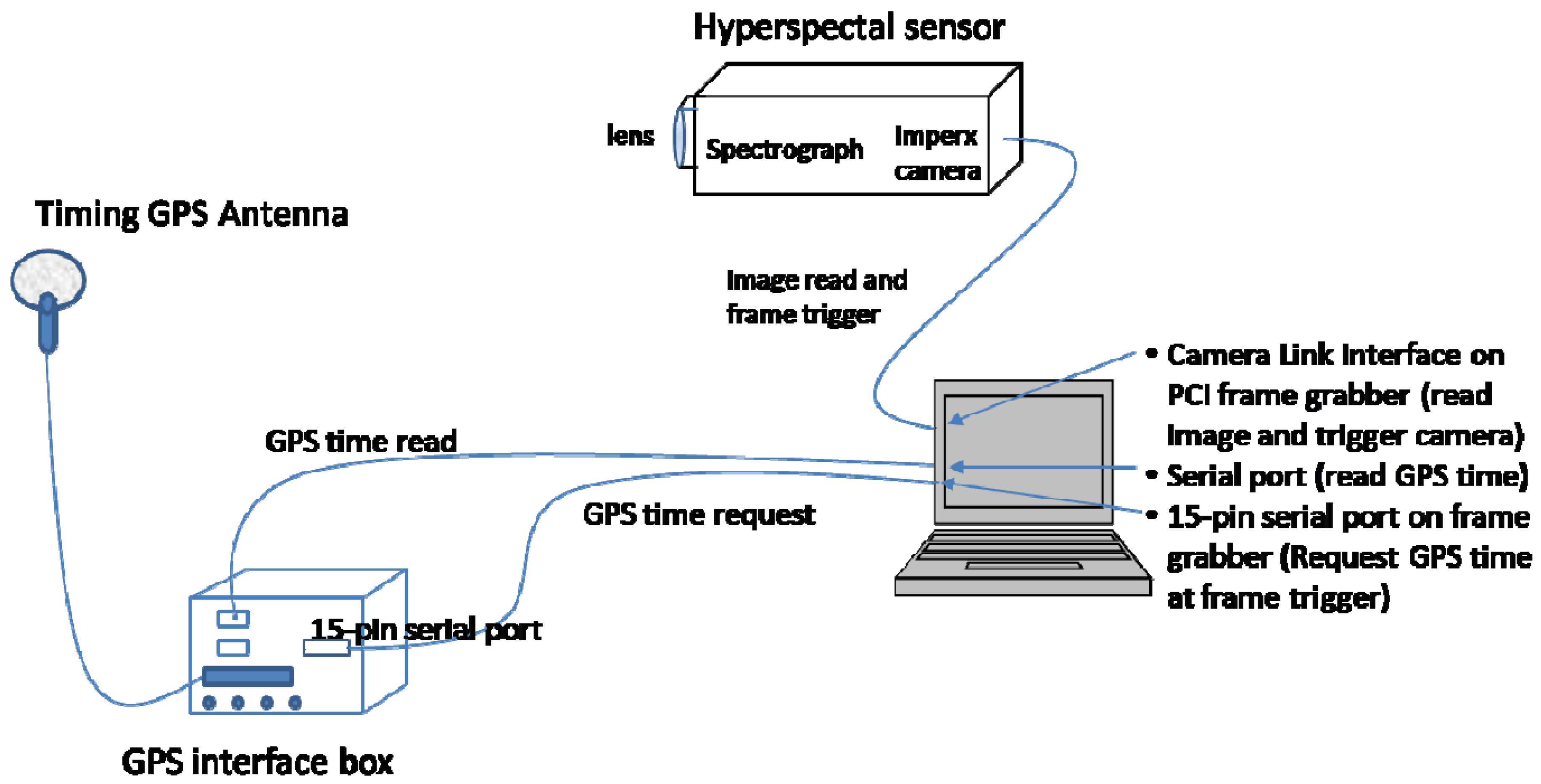
Several design criteria were established to develop the VMMS system as a multi-purpose research and educational tool. One of these criteria was to use off-the-shelf components in a modular interoperable design. Interoperability was important so that the system can be used with multiple platforms utilizing different navigation sensor configurations. The VMMS system is composed of loosely integrated off-the-shelf components that can be divided into two groups: (i) imaging and synchronization sensors; and (ii) navigation sensors. The imaging component is composed of a hyperspectral sensor and consumer-grade high-resolution digital camera(s). Images taken by these sensors are synchronized to the trajectory data through GPS time. The GPS-based synchronization signal is acquired through a designated timing GPS receiver that is different from the geodetic-grade GPS receiver used for determining the platform trajectory. This configuration provides system modularity by allowing the imaging sensors to be georeferenced using different types of position/navigation sensors. Figure 1 presents the main components involved in the hyperspectral and digital camera image acquisition and synchronization process. Detailed description of these components and their functionalities is presented in the next sub-sections.

Figure 1. Data acquisition components for the hyperspectral sensor (top) and the digital cameras (bottom).

Figure 1. Data acquisition components for the hyperspectral sensor (top) and the digital cameras (bottom).

2.1. Hyperspectral Sensor

The hyperspectral sensor is composed of a V10E Specim ImSpector holographic grating [27], manufactured by Spectral Imaging Ltd (Finland). The grating spectrograph disperses the energy passing through a Schneider-Kreuznach Xenoplan (focal length = 17 mm; f-stop = 1.4) c-mount lens and entering a 30 micron width slit into different wavelengths. The dispersed energy is received by a digital camera attached to the back of the spectrograph. Several off-the-shelf digital cameras can be used in this setup. In our system, an Imperx IPX-2M30H-L was used and installed by Autovision Inc. (http://www.autovision.net/). 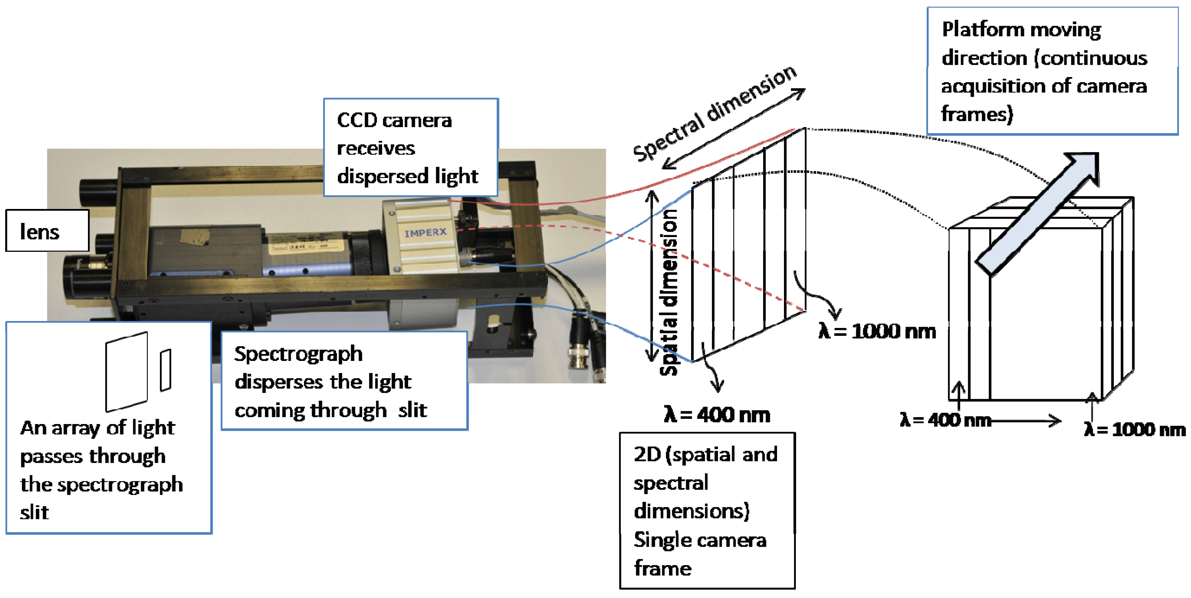Table 1 lists the basic specifications of the V10E ImSpector spectrograph and the Imperx IPX 2M30H-L camera. The energy entering the spectrograph slit is dispersed through the spectrograph optics into different wavelengths and captured by the Imperx camera’s two‑dimensional Charge-Coupled Device (CCD). One dimension on the CCD represents the spatial component and the other dimension represents the spectral component. Each image captured by the Imperx camera represents a line in the formed hyperspectral image. Images are built up line-by-line so that adjacent lines captured by the moving sensor form a hyperspectral image cube. Figure 2 shows a schematic diagram of the hyperspectral image data formation including light dispersion, frame acquisition by the digital camera and image formation through sensor mobility.

The V10E ImSpector spectrograph has a spectral range of 400–1,000 nm with 2.8nm spectral resolution. The Imperx camera has a spectral response range of 400–1,000 nm and a CCD resolution of 1,920 × 1,080 pixels. The spatial dimension of the CCD (1,920 pixels) is binned by two (i.e., each two pixels give one value to achieve higher signal to noise ratio). In our implementation, we acquire 800 pixels in the spatial dimension. The reduced spatial dimension, compared to the physical CCD size of the Imperx camera, even after applying the binning ratio, is to avoid pixels at the edges of the image, which suffer from low incident energy caused by the design of the light dispersing optics.

Table 1. ImSpector Spectrograph and Imperx camera characteristics.

ImSpector V10E Optical Characteristics		Imperx IPX 2M30H-L Camera Characteristics
Spectral range	400–1,000 nm	Active image pixels	1,920 (H) × 1,080 (V)
Spectral resolution	2.8 nm	Active image area	15.9 mm × 8.61 mm
Image size	max 6.15 (spectral) × 14.2 (spatial) mm	Pixel size	7.4 μm
Spatial resolution	rms spot radius < 9 μm	Output	8/10/12 bit
Aberrations	No astigmatism	Interface	Camera link
Bending of spectral lines across spatial axis	Smile < 1.5 μm	Frame rate	33 fps (higher with binning and AOI)
Bending of spatial lines	Keystone < 1 μm	Video gain	6–40 db
Numerical aperture	F/2.4	Hardware/software trigger	Yes
Slit width	30 μm	S/N	60 db
Slit height	14.2 μm	Strobe output	Yes
		Lens mount	C mount 1″ format
		Min illumination	1.0 Lux, f = 1.4

Table 1. ImSpector Spectrograph and Imperx camera characteristics.

ImSpector V10E Optical Characteristics		Imperx IPX 2M30H-L Camera Characteristics
Spectral range	400–1,000 nm	Active image pixels	1,920 (H) × 1,080 (V)
Spectral resolution	2.8 nm	Active image area	15.9 mm × 8.61 mm
Image size	max 6.15 (spectral) × 14.2 (spatial) mm	Pixel size	7.4 μm
Spatial resolution	rms spot radius < 9 μm	Output	8/10/12 bit
Aberrations	No astigmatism	Interface	Camera link
Bending of spectral lines across spatial axis	Smile < 1.5 μm	Frame rate	33 fps (higher with binning and AOI)
Bending of spatial lines	Keystone < 1 μm	Video gain	6–40 db
Numerical aperture	F/2.4	Hardware/software trigger	Yes
Slit width	30 μm	S/N	60 db
Slit height	14.2 μm	Strobe output	Yes
		Lens mount	C mount 1″ format
		Min illumination	1.0 Lux, f = 1.4

Figure 2. A schematic diagram showing hyperspectral image formation.

Figure 2. A schematic diagram showing hyperspectral image formation.

The spectral dimension of each captured frame (1,080 pixels) can be binned by a factor of 4 or 8 to produce 270 or 135 bands, respectively. Using this setting, the dimensions of each captured frame are 800 × 270 or 800 × 135 (depending on the spectral binning factor), which represents a single line in the final hyperspectral image. Adjacent lines (successive frames) captured along platform trajectory produce the final hyperspectral image cube, which has 800 spatial pixels (samples), 270 or 135 bands and a number of lines that depends on the acquisition time and frame rate. A National Instrument (http://www.ni.com/) PCI 1,426 frame grabber is used to trigger the Imperx camera and acquire frames successively. Custom hardware circuit board and software application were developed to control the image acquisition mechanism including the camera synchronization with GPS time.

2.2. Digital Camera(s)

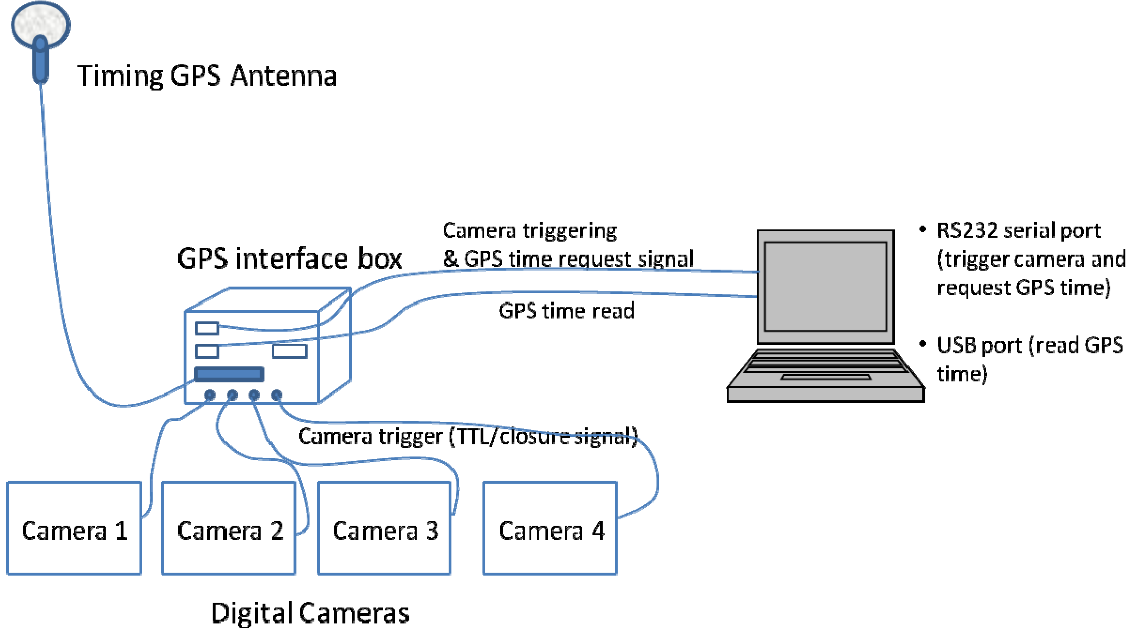
In our implementation, we used a high resolution consumer-grade digital camera system to acquire images in addition to the hyperspectral sensor for documentation and feature recognition purposes. Capturing images with suitable overlap (more than 50%) can allow the creation of 3D models through bundle adjustment of the acquired images [28]. The system can utilize any digital camera that can be triggered by external TTL signal. In our design, a camera trigger signal sent by the acquisition software through the RS232 port is received by a custom electronic circuit that diverts the signal to the camera(s) and the timing GPS. This implementation allows triggering multiple cameras simultaneously, while obtaining a single GPS time stamp for the triggering signal.

2.3. Synchronization (Timing) Sensor

Each imaging sensor (hyperspectral sensor and digital camera(s)) is synchronized independently using GPS time. Synchronization is accomplished using Trimble (http://www.trimble.com/) Accutime Gold^TM GPS receiver, which is capable of responding with a time stamp to an external event within ~500 nanoseconds (ns) from the event arrival [29]. This receiver also outputs a pulse-per-second signal and time stamp with an accuracy of 15 ns at one sigma confidence level. For modularity purposes, two separate Accutime Gold antennas were configured for mobile applications as suggested in the user guide and used in our system for the hyperspectral sensor and the digital camera(s). Design of the image synchronization implementation is detailed in Section 3.

2.4. Navigation Sensors

Many georeferencing techniques that utilize multiple navigation sensor types have been suggested for mobile mapping applications. Systems that integrate satellite positioning systems (e.g., GPS and GLONASS) with tactical grade Inertial Navigation Systems (INS) are most common yet expensive. Recent research suggests that low-cost Micro-Electro-Mechanical Systems (MEMS) IMU have the potential to provide attitude accuracy suitable for some applications. As a low-cost system, the VMMS system utilizes a Gladiator LandMark20 GPS/IMU MEMS-based IMU (http://www.gladiatortechnologies.com/) and Topcon HyperLite+ (http://www.topconpositioning.com/) dual frequency GPS receivers capable of collecting data at 10 Hz rate. We are also in the process of acquiring and testing the higher-grade SPN^TM CPT GPS/INS system from NovAtel (http://www.novatel.com/). Reports of testing the use of low-end MEMS based IMU sensor in ground‑based mobile mapping systems indicated the possibility of achieving a positional accuracy of 0.05 m and attitude accuracy of 0.35 deg [30]. We expect our system to perform much better given the published specs of the Gladiator (MEMS) system.

3. Image Acquisition Software

Two software applications were developed to acquire the hyperspectral and digital camera images and to assign GPS time stamps from our timing GPS receivers using the LabView v8.6 software (http://www.ni.com/labview/). Custom-made electronic boards were developed to support the image synchronization process by passing signals to the timing GPS receivers when an image is triggered. Hardware electronic signals are used to trigger the imaging sensors and to stimulate the GPS receivers simultneously. Detailed information about the software and electronic boards can be acquired through direct contact with the authors.

For the hyperspectral sensor, the application simultaneously triggers the camera and sends a hardware signal to an electronic board that directs this signal to the timing GPS receiver. The receiver responds back with a time stamp that is recorded by the application, which also acquires the captured frames, reformats and stores them in Binary Interlaced by Line (BIL) format. The data transfer communication with the timing receiver is conducted using serial communication (9,600 bits per second baud rate) through the proprietary Trimble Standard Interface Protocol (TSIP). Binary data packets sent by the receiver (including GPS time) in response to hardware sensor trigger events are received, parsed and stored by the application. The application also implements a buffer queue algorithm for image data acquisition to ensure continuous image recording and minimize frame dropping.

Figure 1 illustrates the hyperspectral system components and their functions. A series of trigger signals are created by the acquisition application and sent through the camera link interface on the frame grabber to the Imprex camera. These triggers are synchronized with hardware pulses sent to the custom-made GPS interface board through a 15-pin serial port on the frame grabber. The pulses are received by the timing GPS receiver, which responds by sending time stamps that correspond to the triggered frames. This implementation creates a hardware trigger mechanism that is robust against delay introduced by the operating system delay. Each frame captured by the Imperx camera represents a single line in the final hyperspectral image. This mandates a fast acquisition rate to maintain continuous object coverage. In the mean time, the Trimble Accutime Gold GPS receiver can time stamp events up to 5 Hz. In the VMMS implementation, a maximum of 5 frames per second are synchronized through the Accutime GPS receiver. An interpolation algorithm estimates the time up to the maximum number of frames captured by the Imperx camera.

A different application was developed for the consumer-grade camera(s) image acquisition and synchronization with GPS time. The application utilizes hardware triggering signals created at certain frequency and sent to the camera and the timing GPS receiver through RS232 port. This simple and generic implementation allows the application to run from any laptop computer with RS232 port and is capable of handling multiple cameras at the same time.

4. Radiometric and Spectral Characteristics of Hyperspectral Sensor

4.1. Radiometric Characteristics

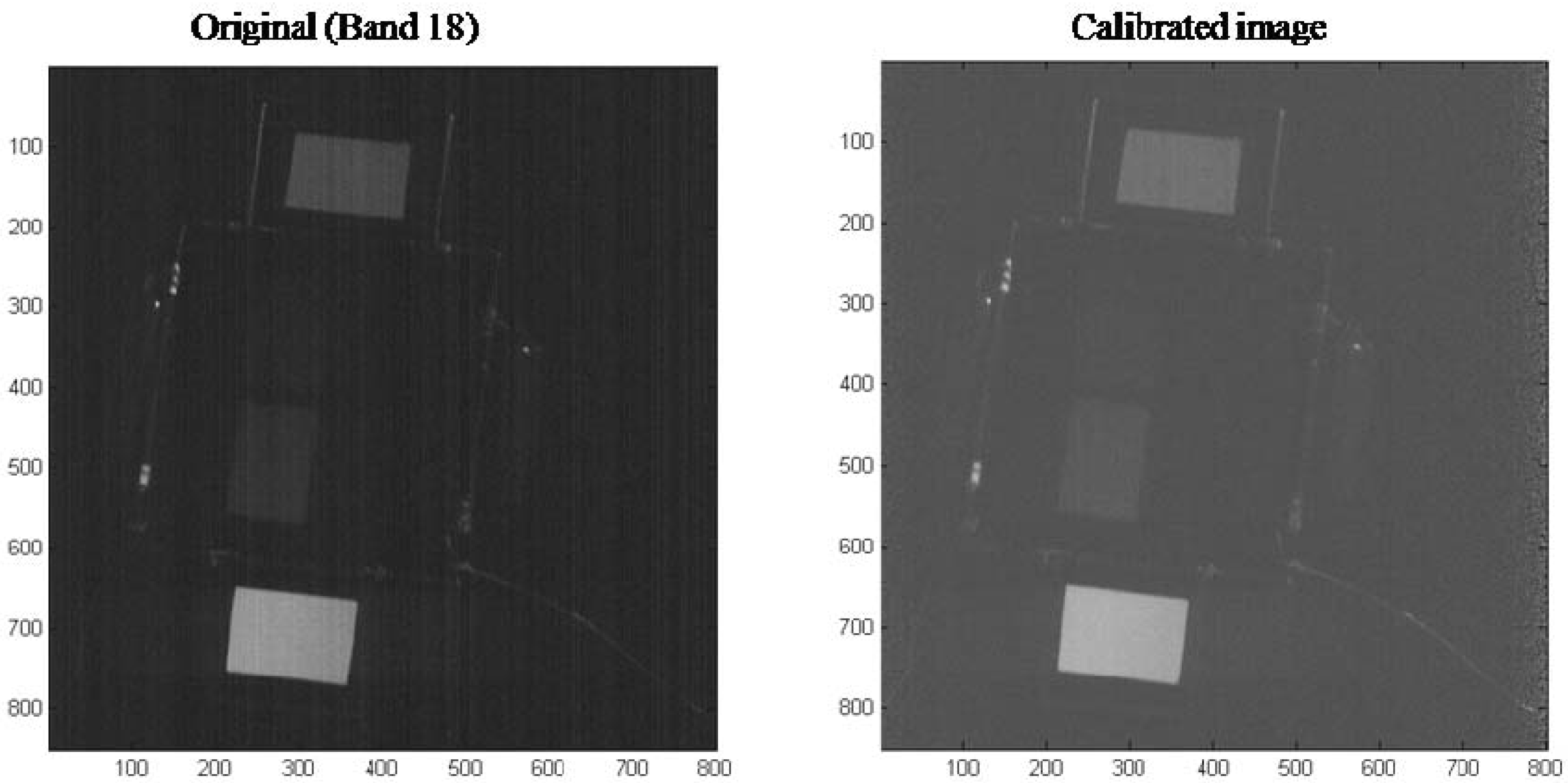
The Imperx digital camera captures images with 12 bit radiometric resolution using CCD sensor technology. Individual CCD pixels produce signal known as dark current even if they are not exposed to light. Dark currents are corrected by collecting a dark cube image while the sensor is not receiving light. Dark values are then subtracted from the digital number values of each image pixel. Additionally, pixels on the sensor may have different gain and offset components when reacting to incident photons. Binning reduces the effect of gain and offset differences by integrating detector response over multiple pixels. Remaining artifacts, however, are usually evidenced by a striping appearance of treated images, especially over homogeneous objects.

We performed several tests to determine the relative gain and offset characteristics of each pixel. The detectors’ relative calibration coefficients were determined by analyzing reference images taken of homogeneous targets at different light intensities. A total of 6 images of white and black targets (Spectralon targets with 99% and 1% calibrated reflectance) were captured by the sensor in direct sunlight with different exposure time settings. All pixel digital numbers were normalized to the mean of the middle 50%. For each image band captured using N = 800 detectors (pixels), the observation equation that models the linear gain a and offset b coefficients as a function of observed DN^o and calibrated DN^c digital numbers can be written as:

$$D{N}_i^{o,k}=a^k\times D{N}_i^{c,k}+b^k+v_i^k$$

(1)

where, i = 1, 2, …L is the line in a single image band; k = 1, 2, ….N = 800 is the detector (pixel) number in a single band line; $D{N}_i^{o,k}$ is the observed DN value, $D{N}_i^{c,k}$ is the calibrated DN value; and $v_i^k$ is the residual error.

Figure 3 shows bands 10 (heavy stripes) and 18 (moderate stripes) of an image cube taken before and after applying the gain and offset calibration coefficients. The image shows that the appearance of striping was greatly reduced.

Figure 3. The results of applying relative detector calibration on band 10 (top) and band 18 (bottom) of one of the hyperspectral images captured by our sensor for a water body with floating and submerged reflection sheets.

Figure 3. The results of applying relative detector calibration on band 10 (top) and band 18 (bottom) of one of the hyperspectral images captured by our sensor for a water body with floating and submerged reflection sheets.

4.2. Spectral Characteristics

As previously mentioned, one dimension of the frame captured by the Imperx camera is binned by a factor of 2 (spatial dimension), while the other dimension is binned by either 4 or 8 (spectral dimension). A total of 270 and 135 spectral bands (effective 205, and 102) can be achieved if the binning modes are 4 and 8, respectively. A binning mode of 8 reduces the size of the image and enhances the signal to noise ratio at the expense of reduced spectral resolution. An approximate empirical calibration algorithm was used to determine the wavelength range for each band. The algorithm utilized the characteristics of the Fluorescent light and fit a linear regression model between the band numbers and the corresponding wavelengths as shown in Figure 4.

Figure 4. Empirical spectral calibration using Fluorescent light spectra (8 pixel spectral binning configuration). Fluorescent light spectra (left) and linear regression of wavelength against band number (right).

Figure 4. Empirical spectral calibration using Fluorescent light spectra (8 pixel spectral binning configuration). Fluorescent light spectra (left) and linear regression of wavelength against band number (right).

5. Ground Pixel Size

Two components govern the spatial resolution of our system. In the across-track direction, spatial resolution is determined by the binned pixel(s) size (px = 2 × 7.4 = 14.8 microns), lens focal length (f = 17 mm), and the distance between the sensor and object. In the along-track direction, spatial resolution is determined by the spectrograph slit size (s = 30 microns), lens focal length and distance from the imaged object determine the system spatial resolution. The ground pixel size in the across-track (w_c) and along-track (w_l) directions are shown by Equations (2) and (3).

$$w_c = px*\frac{H}{f}$$

(2)

$$w_l= s*\frac{H}{f}$$

(3)

where H is the distance between the sensor and the imaged object.

Equation (4) depicts total across-track ground coverage (W_c) by multiplying the pixel ground coverage (w_c) by the number of pixels in each line (S = 800 pixels). Spacing between two consecutive along track lines (W_l) is determined by the speed (v) of the mobile platform (ground or air vehicle) and the capturing frame rate (r) as shown in Equations (5).

$$W_c = S*w_c$$

(4)

$$W_l= \frac{v}{r}$$

(5)

In order to attain continuous along track coverage, the distance $W_l$ should not exceed the distance $w_l$. This is achieved by controlling the platform speed, acquisition rate and/or the distance between the sensor and the objet. In our system, frame rate is adjustable through the image acquisition software as described in Section 3.1. Table 2 lists along-track and across-track track coverage at different distances from the imaged objects, platform speeds, and acquisition frame rates (20, 40, and 60 frame per second).

Table 2. Hyperspectral sensor spatial coverage at different vehicle speeds and frame acquisition rates.

Frame rate r (frames/second)	20 frames/sec
max speed v (m/sec)	0.3	0.4	0.5	3	4	5	50	60	70
Along track distance between lines wl (cm)	1.5	2.0	2.5	15.0	20.0	25.0	250.0	300.0	350.0
Minimum distance to object H (m)	8.5	11.3	14.2	85.0	113.3	141.7	1,416.7	1,700.0	1,983.3
Across track pixel size wa (cm)	0.7	1.0	1.2	7.4	9.9	12.3	123.3	147.9	172.6
Across track ground coverage Wa (m)	5.9	7.9	9.9	59.2	78.9	98.6	986.0	1,183.2	1,380.4
Frame rate r (frames/second)	40 frames/sec
max speed v (m/sec)	0.3	0.4	0.5	3	4	5	50	60	70
Along track distance between lines wl (cm)	0.8	1.0	1.3	7.5	10.0	12.5	125.0	150.0	175.0
Minimum distance to object H (m)	4.3	5.7	7.1	42.5	56.7	70.8	708.3	850.0	991.7
Across track pixel size wa (cm)	0.4	0.5	0.6	3.7	4.9	6.2	61.6	74.0	86.3
Across track ground coverage Wa (m)	3.0	3.9	4.9	29.6	39.4	49.3	493.0	591.6	690.2
Frame rate r (frames/second)	60 frames/sec
max speed v (m/sec)	0.3	0.4	0.5	3	4	5	50	60	70
Along track distance between lines wl (cm)	0.5	0.7	0.8	5.0	6.7	8.3	83.3	100.0	116.7
Minimum distance to object H (m)	2.8	3.8	4.7	28.3	37.8	47.2	472.2	566.7	661.1
Across track pixel size wa (cm)	0.2	0.3	0.4	2.5	3.3	4.1	41.1	49.3	57.5
Across track ground coverage Wa (m)	2.0	2.6	3.3	19.7	26.3	32.9	328.7	394.4	460.1

Table 2. Hyperspectral sensor spatial coverage at different vehicle speeds and frame acquisition rates.

Frame rate r (frames/second)	20 frames/sec
max speed v (m/sec)	0.3	0.4	0.5	3	4	5	50	60	70
Along track distance between lines wl (cm)	1.5	2.0	2.5	15.0	20.0	25.0	250.0	300.0	350.0
Minimum distance to object H (m)	8.5	11.3	14.2	85.0	113.3	141.7	1,416.7	1,700.0	1,983.3
Across track pixel size wa (cm)	0.7	1.0	1.2	7.4	9.9	12.3	123.3	147.9	172.6
Across track ground coverage Wa (m)	5.9	7.9	9.9	59.2	78.9	98.6	986.0	1,183.2	1,380.4
Frame rate r (frames/second)	40 frames/sec
max speed v (m/sec)	0.3	0.4	0.5	3	4	5	50	60	70
Along track distance between lines wl (cm)	0.8	1.0	1.3	7.5	10.0	12.5	125.0	150.0	175.0
Minimum distance to object H (m)	4.3	5.7	7.1	42.5	56.7	70.8	708.3	850.0	991.7
Across track pixel size wa (cm)	0.4	0.5	0.6	3.7	4.9	6.2	61.6	74.0	86.3
Across track ground coverage Wa (m)	3.0	3.9	4.9	29.6	39.4	49.3	493.0	591.6	690.2
Frame rate r (frames/second)	60 frames/sec
max speed v (m/sec)	0.3	0.4	0.5	3	4	5	50	60	70
Along track distance between lines wl (cm)	0.5	0.7	0.8	5.0	6.7	8.3	83.3	100.0	116.7
Minimum distance to object H (m)	2.8	3.8	4.7	28.3	37.8	47.2	472.2	566.7	661.1
Across track pixel size wa (cm)	0.2	0.3	0.4	2.5	3.3	4.1	41.1	49.3	57.5
Across track ground coverage Wa (m)	2.0	2.6	3.3	19.7	26.3	32.9	328.7	394.4	460.1

6. Sample Data Collection and Preliminarily Analysis

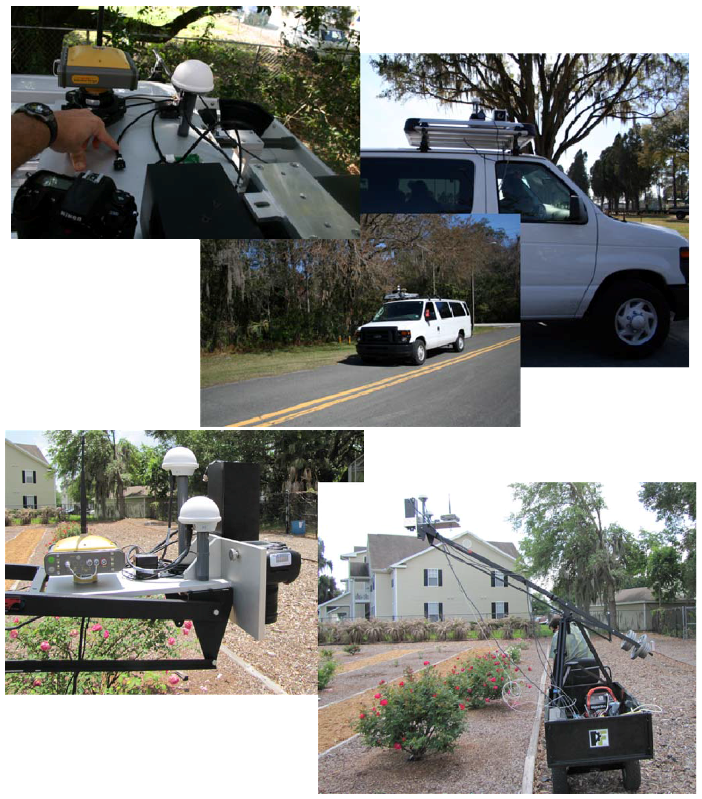
Our VMMS system was designed to fit two different ground-based mobile platforms: one for road right-of-way mapping and the other for precision agriculture applications. The system can be mounted on a motor vehicle (van) so that the cameras look to the side at the right-of-way objects. The precision agriculture imaging application was facilitated by mounting the imaging and navigation devices on a plate positioned on a crane. The crane tripod can be carried by a truck or a tractor. In this design, the cameras look downwards for vegetation (e.g., crop) imaging. Figure 5 shows the imaging and navigation equipment mounted on both platforms.

An image of a road right-of-way captured by the hypersepctral sensor mounted on the roof of a van is shown in Figure 6. The image is formed line-by-line with vehicle movement. A false color representation is shown in the figure using three of the hyperspectral image narrow bands (R:765 nm, G:683 nm, B:552 nm). The figure also shows the spectral profile captured by the sensor for three different locations on the image for a healthy shrub, dead grass, and the sky.

Figure 5. Imaging system mounted on a van (top) and on a boom carried by a tractor trailer (bottom).

Figure 5. Imaging system mounted on a van (top) and on a boom carried by a tractor trailer (bottom).

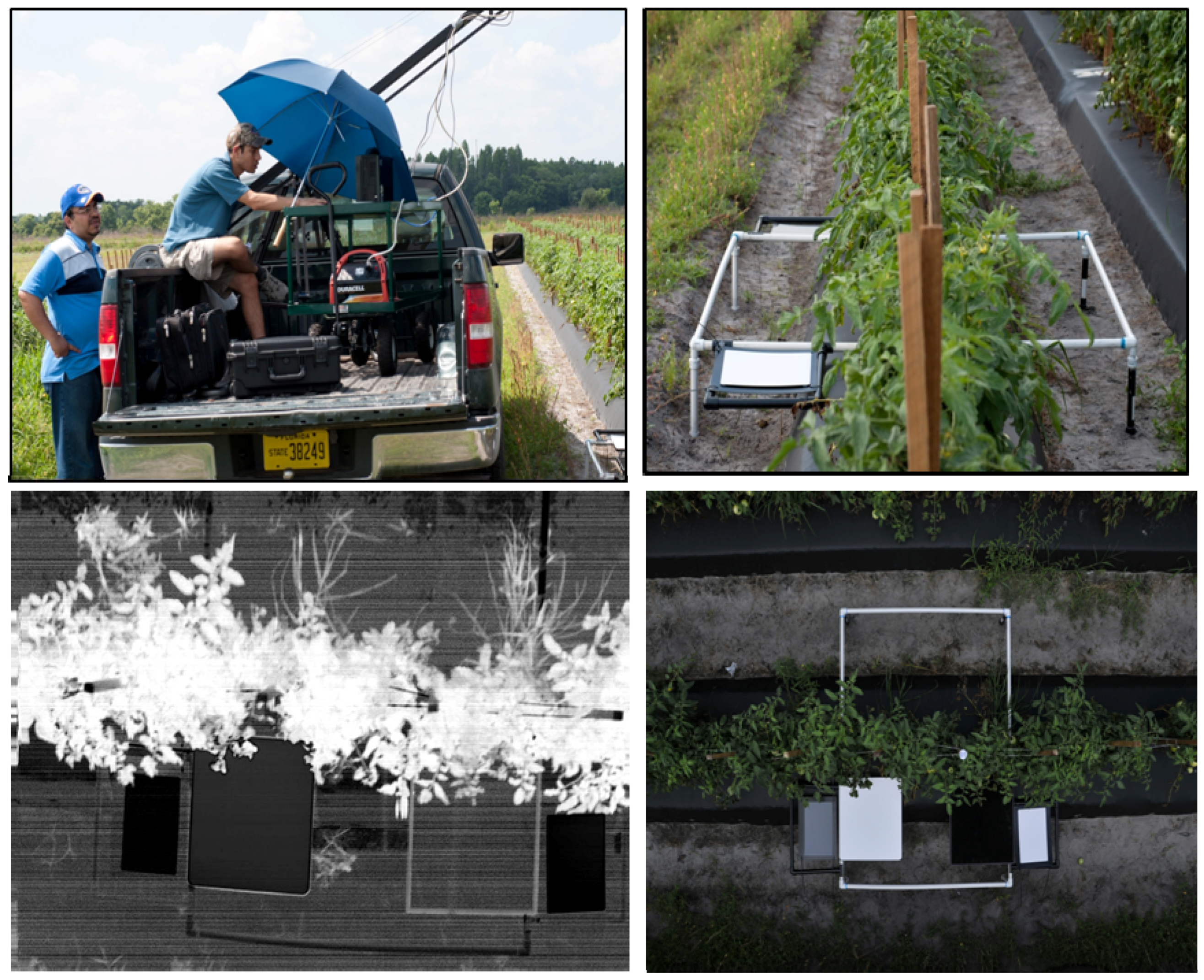
Two data sets were analyzed by our system to: (1) quantify tomato vegetation health and (2) estimate chlorophyll-a (chl-a) concentration in aquaculture ponds. The algorithms used in the analysis used individual narrow bands acquired by our hyperspectral sensor in the red and infrared regions of the spectrum. The tomato vegetation experiment was conducted to evaluate the use of our systems to detect and quantify bacterial disease in tomato vegetation. Our experiments involved capturing imagery on three different dates along the plant cycle at 4, 6, and 8 weeks age for five different trials under different management conditions and was accompanied by field evaluation accomplished by plant pathology experts. Figure 7 shows image acquisition of tomato field and calibration boards used for the image atmospheric calibration. The bottom left corner image is an image subset of a Normalized Difference Vegetation Index (NDVI) using two bands (λ = 668 and 736 nm).

Figure 6. False color (R:765 nm, G:683 nm, B:552 nm) (top) composite for right-of-way vegetation captured using van-mounted hyperspectral sensor. Spectral profiles (bottom) for healthy vegetation, stressed vegetation and the sky.

Figure 6. False color (R:765 nm, G:683 nm, B:552 nm) (top) composite for right-of-way vegetation captured using van-mounted hyperspectral sensor. Spectral profiles (bottom) for healthy vegetation, stressed vegetation and the sky.

Our initial evaluation used the NDVI calculated using two bands (λ = 668 and 736 nm). These two bands represent the chlorophyll-a strong absorption and fluorescence bands in the red and infrared region and define the two end of the chlorophyll red edge area of the spectrum. Although, we used NDVI index only in this preliminarily phase, the results quantified plant growth in the plant from edge 4 to 6 weeks, which overcame the disease effect. The plant at age 8 weeks showed clear deterioration and produced a correlation of 0.60 with field estimation. Future experiments are underway to use other plant indices, refine used wavelengths, and to create models that take plant growth into consideration.

In the second experiment (water quality analysis), the images were acquire simultaneously with water samples from 30 aquaculture ponds to study the feasibility of using ground-based remote sensing sensors in estimating chl-a concentration in the water as indicator of algae bloom and a measure of water quality. A 3-band index [6] utilizing bands (λ = 680, 700 and 769 nm) produced a correlation coefficient of 0.93 with chl-a concentration obtained by lab analysis of water samples. Work is still undergoing to improve the chl-a estimation model using submerged targets and to extend the model to other water quality parameters such as Nitrogen and Phosphorus content.

Figure 7. Image acquisition of Tomato field. Bottom left image shows NDVI created using the λ = 668 and 736 nm bands.

Figure 7. Image acquisition of Tomato field. Bottom left image shows NDVI created using the λ = 668 and 736 nm bands.

7. Summary and Conclusions

A low-cost hyperspectral imaging system composed of an integrated set of off-the-shelf imaging and navigation sensors was demonstrated. Our system is comprised of a spectrograph to disperse light spectrally, digital camera to capture light dispersed by the spectrograph, consumer-grade digital camera for documentation and low accuracy positioning analysis, GPS timing receiver(s) to synchronize captured frames with GPS time, and navigation sensors (positioning GPS receiver and IMU) for trajectory and attitude observation. The system can be mounted on multiple platforms to provide images at multiple scales and various applications. Two ground-based implementations were presented for right-of-way mapping and cultivated crop studies. A modular system design was adopted that separates the imaging component from the positioning and attitude measuring components. This design allows the imaging system to be interoperable through use with different positioning and attitude systems. Captured frames were triggered and simultaneously synchronized with GPS time through designated GPS timing receivers. Radiometric calibration was achieved by normalizing pixel gain and offset response of individual pixels. An empirical method for spectral calibration that utilizes the spectrum properties for Fluorescent light was used to estimate band wavelengths. The utility of our system was demonstrated through preliminarily analysis of images captured for aquaculture ponds and tomato vegetation.

For future research, we envision the need to finalize testing the overall positional accuracy of the system using different navigation sensors. On the application side, efforts are needed to develop atmospheric calibration procedures for the hyperspectral imagery to incorporate variations in sensor‑object-sun locations along extended road segments and to account for shadow effect and variations in object scales due to varying object-senor distances.

References and Notes

- Lu, D.; Weng, Q. A survey of image classification methods and techniques for improving classification performance. Int. J. Remote Sens. 2007, 28, 823–870. [Google Scholar] [CrossRef]
- Champagne, C.; Staenz, K.; Bannari, A.; Deguise, J.-C.; Mcnairn, H.; Shang, S. Validation of a Hyperspectral Curve-Fitting Model for the estimation of plant water content of agricultural canopies. Remote Sens. Environ. 2003, 87, 148–160. [Google Scholar] [CrossRef]
- Okamoto, H.; Murata, T.; Kataoka, T.; Hata, S. Plant classification for weed detection using hyperspectral imaging with wavelet analysis. Weed Biol. Manag. 2007, 7, 31–37. [Google Scholar] [CrossRef]
- Koponen, S.; Pulliainen, J.; Kallio, K.; Hallikainen, M. Lake water quality classification with airborne hyperspectral spectrometer and simulated MERIS data. Remote Sens. Environ. 2002, 79, 51–59. [Google Scholar] [CrossRef]
- Thiemann, S.; Kaufmann, H. Lake water quality monitoring using hyperspectral airborn data—A semiempirical multisensor and multitemporal approach for the Mecklenburg Lake District, Germany. Remote Sens. Environ. 2002, 81, 228–237. [Google Scholar] [CrossRef]
- Gitelson, A.A.; Dall’Olmo, G.; Moses, W.; Rundquist, D.C.; Barrow, T.; Fisher, T.R.; Gurlin, D.; Holz, J. A simple semi-analytical model for remote estimation of chlorophyll-a in turbid waters: Validation. Remote Sens. Environ. 2008, 112, 3582–3593. [Google Scholar] [CrossRef]
- Estep, L.; Terrie, G.; Davis, B. Technical Note: Crop stress detection using AVIRIS hyperspectral imagery and artificial neural networks. Int. J. Remote Sens. 2004, 25, 4999–5004. [Google Scholar] [CrossRef]
- Ye, X.; Sakai, K.; Garciano, L.; Asada, S.; Sasao, A. Estimation of citrus yield from airborne hyperspectral images using a neural network model. Ecol. Model. 2006, 198, 426–432. [Google Scholar] [CrossRef]
- Schmidt, K.S.; Skidmore, A.K. Spectral discrimination of vegetation types in a coastal wetland. Remote Sens. Environ. 2003, 85, 92–108. [Google Scholar] [CrossRef]
- Becker, B.L.; Lusch, D.P.; Qi, J. Identifying optimal spectral bands from in situ measurements of Great Lakes coastal wetlands using second derivative analysis. Remote Sens. Environ. 2005, 97, 238–248. [Google Scholar] [CrossRef]
- Porter, W.M.; Enmark, H.T. A system overview of the Airborne Visible/Infrared Imaging Spectrometer (AVIRIS). Proc. SPIE 1988, 834, 22–31. [Google Scholar]
- Vane, G.; Green, R.O.; Chrien, T.G.; Enmark, H.T.; Hansen, E.G.; Porter, W.M. The airborne visible/infrared imaging spectrometer (AVIRIS). Remote Sens. Environ. 1993, 44, 127–143. [Google Scholar] [CrossRef]
- Cocks, T.; Jenssen, R.; Stewart, A.; Wilson, I.; Shields, T. The HyMap Airborne Hyperspectral Sensor: The System, Calibration and Performance. In Proceedings of 1st EARSeL Workshop on Imaging Spectroscopy, Zurich, Switzerland, 6–8 October 1998; pp. 37–43.
- Anger, C.D.; Mah, S.; Babey, S.K. Technological Enhancements to the Compact Airborne Spectrographic Imager (CASI). In Proceedings of 1st International Airborne Remote Sensing Conference and Exhibition, Strasbourg, France, 11–15 September 1994; Volume 2, pp. 200–213.
- Oppelt, N.; Mauser, W. Airborne Visible/Infrared Imaging Spectrometer AVIS: Design, characterization and calibration. Sensors 2007, 7, 1934–1953. [Google Scholar] [CrossRef] [Green Version]
- Basedow, R.W.; Carmer, D.C.; Anderson, M.E. HYDICE System: Implementation and performance. Proc. SPIE 1995, 2480, 258–267. [Google Scholar]
- Pearlman, J.S.; Barry, P.S.; Segal, C.; Shepanski, J.; Beiso, D.; Carman, S. Hyperion, A space‑based imaging spectrometer. IEEE Trans. Geosci. Remote Sens. 2003, 41, 1160–1173. [Google Scholar] [CrossRef]
- Mcclure, W.F.; Moody, D.; Stanfield, D.L.; Kinoshita, O. Hand-held NIR spectrometry. Part II: An economical no-moving parts spectrometer for measuring chlorophyll and moisture. Appl. Spectrosc. 2002, 56, 720–724. [Google Scholar] [CrossRef]
- Li, F.; Gnyp, M.L.; Jia, L.; Miao, Y.; Yu, Z.; Koppe, W.; Bareth, G.; Chen, X.; Zhang, F. Estimating N status of winter wheat using a handheld spectrometer in the North China Plain. Field Crops Res. 2008, 106, 77–85. [Google Scholar] [CrossRef]
- Hadley, B.C.; Garcia-Quijano, M.; Jensen, J.R. Empirical versus model-based atmospheric correction of digital airborne imaging spectrometer hyperspectral data. Geocarto Int. 2005, 20, 21–28. [Google Scholar] [CrossRef]
- Glenn, N.F.; Mundt, J.T.; Weber, K.T.; Prather, T.S.; Lass, L.W.; Pettingill, J. Hyperspectral data processing for repeat detection of small infestations of leafy spurge. Remote Sens. Environ. 2005, 95, 399–412. [Google Scholar] [CrossRef]
- Hummel, J.W.; Sudduth, K.A.; Hollinger, S.E. Soil moisture and organic matter prediction of B‑horizon soils using an NIR soil sensor. Comput. Electron. Agr. 2001, 32, 149–165. [Google Scholar] [CrossRef]
- Kostrzewski, M.; Waller, P.; Guertin, P.; Haberland, J.; Colaizzi, P.; Barnes, E.; Thompson, T.; Clarke, T.; Riley, E.; Choi, C. Ground-based remote sensing of water and nitrogen. Trans. ASAE 2003, 46, 29–38. [Google Scholar] [CrossRef]
- Downey, G.; Fouratier, V.; Kelly, J.D. Detection of honey adulteration by addition of fructose and glucose using near infrared transflectance spectroscopy. Near Infrared Spectrosc. 2003, 11, 447–456. [Google Scholar] [CrossRef]
- Okamoto, H.; Lee, W.S. Green citrus detection using hyperspectral imaging. Comput. Electron. Agr. 2009, 66, 201–208. [Google Scholar] [CrossRef]
- Ye, X.; Sakai, K.; Okamoto, H.; Garciano, L.O. A ground-based hyperspectral imaging system for characterizing vegetation spectral features. Comput. Electron. Agr. 2008, 63, 13–21. [Google Scholar] [CrossRef]
- Aikio, M. Hyperspectral Prism-Grating-Prism Imaging Spectrograph. Ph.D. Dissertation, Technical Research Center of Finland, Espoo, Finland, 2001. [Google Scholar]
- Abd-Elrahman, A.; Gad-Elraab, M. Using commercial-grade digital camera in the estimation of hydraulic flume bed changes. Survey. Land Inform. Sci. 2008, 68, 35–45. [Google Scholar]
- Trimble. Trimble Acutime Gold User Guide; 2007; Available online: http://trl.trimble.com/docushare/dsweb/Get/Document-377646/TrimbleAcutimeGold_1A.pdf (accessed on 10 May 2010).
- Niu, X.; Hassan, T.; Ellum, C.; El-Sheimy, N. Directly Georeferencing Terrestrial Imagery Using MEMS-based INS/GNSS Integrated Systems. In Proceedings of the XXIII FIG Congress, Munich, Germany, 8–13 October 2006.
© 2011 by the authors; licensee MDPI, Basel, Switzerland. This article is an open access article distributed under the terms and conditions of the Creative Commons Attribution license (http://creativecommons.org/licenses/by/3.0/).