Estimating Single Tree Stem Volume of Pinus sylvestris Using Airborne Laser Scanner and Multispectral Line Scanner Data

Abstract

So far, only a few studies have been carried out in central European forests to estimate individual tree stem volume of pine trees from high resolution remote sensing data. In this article information derived from airborne laser scanner and multispectral line scanner data were tested to predict the stem volume of 178 pines (Pinus sylvestris) in a study site in the south-west of Germany. First, tree crowns were automatically delineated using both multispectral and laser scanner data. Next, tree height, crown diameter and crown volume were derived for each crown segment. All combinations of the derived tree features were used as explanatory variables in allometric models to predict the stem volume. A model with tree height and crown diameter had the best performance with respect to the prediction accuracy determined by a leave-one-out cross-validation: Root Mean Square Error (RMSE) = 24.02% and Bias = 1.36%.

1. Introduction

In general two main approaches are distinguished to estimate forest inventory attributes from airborne laser scanner (ALS) data [1]: (1) Area based methods, also described as canopy height distribution (CHD) approaches; and (2) Individual-tree-detection (ITD) methods. Often the CHD approaches are associated with low-resolution and the ITD methods with high-resolution data.

In Central Europe, the majority of studies have concentrated on CHD approaches to estimate forest inventory attributes such as stand heights, basal area or timber volume per hectare. Usually geo-referenced plots from operational inventories were utilized as reference data. Metrics related to canopy height and densities have been used as predictors in regression models and nonparametric methods (e.g., [2,3,4,5]).

In addition, a number of single tree delineation algorithms were developed. Possibilities to detect individual tree crowns in deciduous and mixed temperate forests in Germany are described in [6]. In [7] a 3D single tree modeling procedure was developed and tested in a mixed forest in southern Germany. A 3D segmentation technique using full-waveform ALS data was presented by [8]. The procedure was tested in the Bavarian Forest National Park in south-eastern Germany. The potential of full-waveform ALS for tree species classification in a mixed forest in Austria was presented by [9].

However, there are fewer ALS studies in central European forests that explored the estimation of individual-tree-based information relevant for forest inventories such as tree height, stem diameter and stem volume. Experiments have been carried out in the Bavarian Forest National Park in south-eastern Germany [10,11,12]. A first European-wide attempt to derive single tree information from ALS data was carried out within the HIGH-SCAN project [13].

The main reason why CHD approaches have been favored is due to the fact that these methods are considered to be more robust than ITD techniques [14,15]. Particularly in dense deciduous forests in the temperate climate zones it can be difficult to delineate individual trees with satisfying accuracy [6]. Another reason why the estimation of single tree attributes has not been studied in detail is that appropriate reference data is often missing. The positions of trees on the ground have to be measured with high precision. Otherwise it is very difficult and often impossible to link crown segments which were delineated based on remote sensing data with trees measured in the field.

The objective of this study was to analyze the potential of high-resolution ALS and multispectral line scanner data for the extraction of individual-tree-based information for pine trees (Pinus sylvestris) in a study site in the south-west of Germany. The main objective was to assess the accuracy of several allometric models for stem volume estimation of automatically delineated trees. The results were analyzed and compared to other studies carried out in Germany and Scandinavia.

2. Test Site and Data

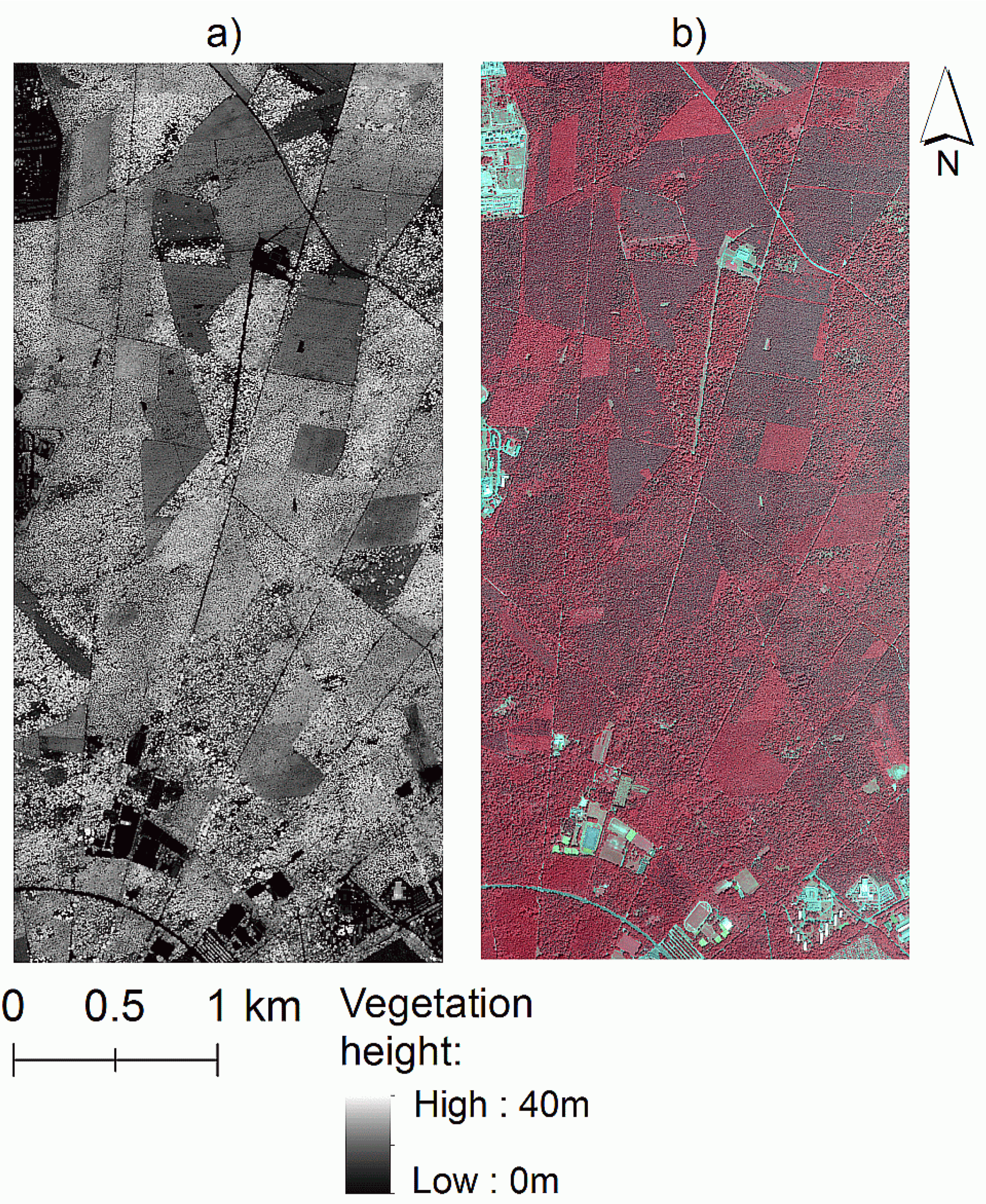
The study area is located in the south-west of Germany, north of the city of Karlsruhe within the federal state of Baden-Württemberg and has a size of 924 ha (Its coordinates in the Gauss–Krüger system are: top left: 3,456,300,00/5,436,100,00 and bottom right: 3,458,400,00/5,431,700,00). A vegetation height model from ALS and a color-infrared (CIR) orthophoto of the study area is shown in Figure 1.

The study site is characterized by flat terrain (min. height: 101 m a.s.l., max. height: 123 m a.s.l.) and various forest stands (pure and mixed forest) with different species and age classes. However, Scots pine (Pinus sylvestris) dominates the study site with 51% (in total 56% coniferous trees).

Figure 1. (a) Vegetation height model from ALS and (b) Color-infrared orthophoto from multispectral line scanner data of the study area near Karlsruhe, Germany.

Figure 1. (a) Vegetation height model from ALS and (b) Color-infrared orthophoto from multispectral line scanner data of the study area near Karlsruhe, Germany.

Four spectral channels were acquired during leaf-on conditions in July 2008 by TopoSys GmbH using a multispectral line scanner. One advantage of this sensor is that shadowing effects only occur orthogonal to the flight line [16]. The single flight strips were rectified and geo-referenced using a surface model, which was filtered from laser scanner data (6–7 points/m²) and acquired at the same time as the optical data. Important flight and technical parameters of the line scanner are listed in Table 1.

Table 1. Flight and technical parameters of the flight campaign in summer 2008 using a multispectral line scanner integrated in the “Falcon II system” (AGL = above ground level).

Parameter	Value
Flying height	700 [m] AGL
Spectral channels	Blue: 450–490 [nm] Green: 500–580 [nm] Red: 580–660 [nm] Near infrared: 770–890 [nm]
Viewing angle	21.6 [°]
Pixels per line	682
Ground sampling distance	0.4 [m]

Table 1. Flight and technical parameters of the flight campaign in summer 2008 using a multispectral line scanner integrated in the “Falcon II system” (AGL = above ground level).

Parameter	Value
Flying height	700 [m] AGL
Spectral channels	Blue: 450–490 [nm] Green: 500–580 [nm] Red: 580–660 [nm] Near infrared: 770–890 [nm]
Viewing angle	21.6 [°]
Pixels per line	682
Ground sampling distance	0.4 [m]

Full-waveform laser scanner data were measured in November 2009 by Milan Geoservice GmbH using the IGI Litemapper 5600 system with a Riegl LMS-Q560 (240 KHz) scanner.

To obtain a high point density (> 20 rays/m²), the study area was flown twice, first in north-south and then in east-west direction. Flight and system parameters are shown in Table 2.

Table 2. Flight and system parameters of the flight campaign in summer 2009 with the “Harrier 56” LiDAR system (AGL = above ground level).

Parameter	Value
Measurement rate	240 [kHz]
Field of view	60 [°]
Flying height	600 [m] AGL
Flying speed	46 [m/s]
Density	22 [rays/m2]
Vertical/horizontal accuracy (excluding GPS errors)*	~0.1/~0.03 [m]

*according to manufacturer information.

Table 2. Flight and system parameters of the flight campaign in summer 2009 with the “Harrier 56” LiDAR system (AGL = above ground level).

Parameter	Value
Measurement rate	240 [kHz]
Field of view	60 [°]
Flying height	600 [m] AGL
Flying speed	46 [m/s]
Density	22 [rays/m2]
Vertical/horizontal accuracy (excluding GPS errors)*	~0.1/~0.03 [m]

*according to manufacturer information.

The full-waveform data was processed using the software “RiANALYZE 560” and was delivered in ASCII format with 3D coordinates of the reflections and additional information such as target number, number of targets in beam, echo signal amplitude and the echo pulse width.

An “Active Surface Algorithm”, implemented in the software “TreesVis” [17] was used to compute a terrain and a surface model (DTM and DSM) with 1-m resolution from the reflections. The algorithm employs the general technique of matching a deformable surface to the laser points by means of energy minimization. To estimate a model of the bare earth (DTM), the surface will be fitted to the points that are considered to be terrain points, which are frequently the lowest points within a defined neighborhood [18]. For the computation of a model including vegetation and buildings, the surface will be fitted to the highest reflections. A normalized DSM (nDSM), in forests often referred to as canopy height model (CHM), was derived as the difference model of DSM and DTM:

nDSM(x,y) = DSM(x,y) − DTM(x,y)

Field measurements were carried out in winter 2009 and spring 2010. Nine square field plots with a size of 30 × 30 m were established within forest stands dominated by Scots pine. Some selected stands have a low proportion of further tree species such as red oak (Quercus rubra), sessile oak (Quercus petraea), beech (Fagus sylvatica) and birch (Betula pendula). Figure 2 shows a 3D view (DSM with CIR texture) of a typical pine stand in the test site with one of the square field plots.

Figure 2. 3D view (DSM with CIR texture) of a typical pine stand in the study area with one of the square field plots (visualized by the white lines).

Figure 2. 3D view (DSM with CIR texture) of a typical pine stand in the study area with one of the square field plots (visualized by the white lines).

Starting from the center of the plots the positions of 288 pines were determined with the help of a TruePulse 360 laser rangefinder. Table 3 shows the mean age of the dominant tree layer and the number of trees measured per plot.

Table 3. Overview of the field plots with the mean age of the dominant tree layer and the number of pines measured in the field.

Plot	Age [years]	Age class*	Number of pines measured in the field
1	28	II	78
2	30	II	87
3	55	III	14
4	55	III	21
5	55	III	27
6	80	IV	14
7	80	IV	19
8	85	V	20
9	123	VII	8

*age classes are defined as: II = 21−40 years, III = 41−60 years, IV = 61−80 years

Table 3. Overview of the field plots with the mean age of the dominant tree layer and the number of pines measured in the field.

Plot	Age [years]	Age class*	Number of pines measured in the field
1	28	II	78
2	30	II	87
3	55	III	14
4	55	III	21
5	55	III	27
6	80	IV	14
7	80	IV	19
8	85	V	20
9	123	VII	8

*age classes are defined as: II = 21−40 years, III = 41−60 years, IV = 61−80 years

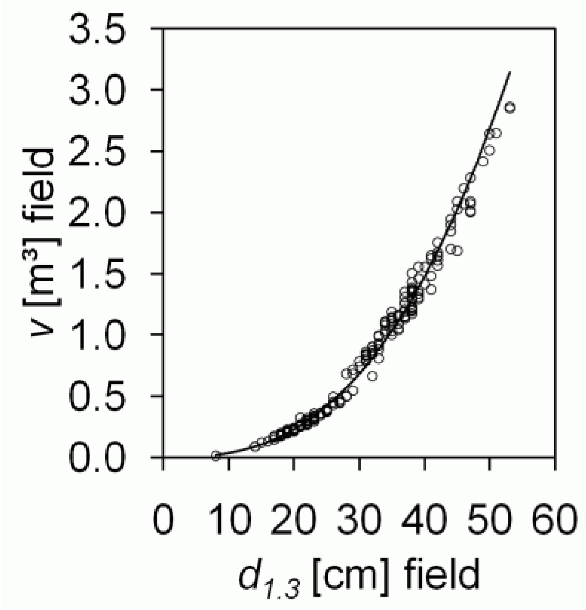
The following features were measured for all trees: (1) height—using a Vertex and (2) diameter at breast height (DBH)—using a caliper. Finally, the stem volume of single trees was computed using the software BDATpro developed by the Forest Research Institute of Baden-Württemberg [19] with the tree height and DBH as the input variables.

3. Methodology

3.1. Automatic Single Tree Segmentation

The processing workflow is a slightly modified version of the algorithm described in [6] and [17]. The main modification is that multispectral line scanner data was integrated in the procedure as an additional dataset with the objective to improve the separation of coniferous and deciduous trees:

• In the first step the study area is classified into the classes: (a) coniferous trees and (b) deciduous trees. For this purpose an unsupervised classification procedure as described in [20] is employed: First, a forest mask is generated using intermediate reflections of the ALS data. Due to the characteristic structure of trees in addition to gaps in the forest canopy, intermediate reflections from branches, stems and leaves between the DSM and DTM can be utilized to delineate the forest area. Inside of the forest mask, gray value combinations of the NIR and green channel of the multispectral line scanner data are used to define a two-dimensional feature space. NIR and green channel were selected, since both channels revealed the main difference in the spectral reflectance of coniferous and deciduous trees in the study site. The assumption is that two distinct clusters can be isolated in the feature space; one represents coniferous trees and the other one deciduous trees. For this purpose the feature space is segmented iteratively until exactly two distinct clusters are generated. After that, pixels of the entire image are classified according to their affiliation to one of the clusters. Next, the definition domain of the study site is reduced to the first class (all regions with coniferous trees).
• In the second processing step individual coniferous tree crowns are segmented based on the DSM from ALS data. DSM based segmentation techniques for crown delineation were suggested by several authors e.g., [21,22,23]. Hypothetically each convex shape in the DSM represents an individual tree crown. The segmentation is achieved with a “pouring algorithm”. The algorithm works similar to “watershed segmentation”. However, for the application of watershed segmentation it is necessary to invert the surface model which is not needed for the pouring segmentation because local maxima are used as the initial points. Local maxima are defined as pixels in the surface model which either alone or as a plateau have higher values than their direct neighbors. Thus, the maxima represent potential tree tops. The boundaries between tree crowns appear as valleys in the surface model. Starting from the maxima regions are expanded down to the deepest points of the valleys as long as there are chains of pixels in which the height values become smaller, similar to water drops flowing downwards in all possible directions [24].
• Due to the fact that the crown segments are often too large, the tree crowns are corrected in the third processing step with the help of a “ray-algorithm”. The assumption is that height changes within an individual crown must be continuous. Thus, virtual rays between the tree tops (local maxima) and border points are generated. New border points are created if there is an interruption in the continuous height changes.

A result of the automatic segmentation is shown in Figure 3. The figure shows a pine stand with age class III (the trees are approximately 55 years old). For better visual interpretation the irregularly shaped crown regions were transformed into circles. Each circle has the same center and the same size as the original crown segment. In Figure 3(a) the automatically delineated pines are superimposed on the nDSM and in Figure 3(b) on a CIR orthophoto. Additionally, in Figure 3(c) the crowns that were measured on the ground, at one of the field plots, are shown as red polygons (eight edges of each crown were projected to the ground using a densitometer).

Figure 3. Automatically delineated pines (yellow circles) with (a) nDSM, (b) CIR orthophoto and (c) crowns measured in the field (red polygons).

Figure 3. Automatically delineated pines (yellow circles) with (a) nDSM, (b) CIR orthophoto and (c) crowns measured in the field (red polygons).

Finally, visual interpretation was used to link automatically delineated crown segments with trees measured on the ground at one of the nine square field plots as listed in Table 3. A tree on the ground was only assigned to an automatically delineated crown if its position was found inside of the crown segment. If more than one tree position was found within a crown segment the tree height was used as an additional criterion. In such a case the tree with the height closest to the ALS measured tree height was assigned. Altogether it was possible to link 178 (61.81%) crown segments with a tree position on the ground. Figure 4 illustrates the number of detected and linked pines in dependence of the age class and Table 4 shows characteristics of the identified trees. The verification result shows only trees that were successfully linked to a corresponding tree position on the ground and which can be used to develop models for volume estimation. Cases where no field tree was found inside an automatically delineated crown are not considered.

Figure 4. Number of detected pines per age class for the field plots listed in Table 3.

Figure 4. Number of detected pines per age class for the field plots listed in Table 3.

Table 4. Characteristics of the 178 identified pine trees.

Variable	Mean	Standard Deviation	Min.	Max.
Height [m]	22.62	5.17	9.80	32.30
Stem diameter [cm]	31.31	9.49	8.00	53.00
Stem volume [m³]	0.9217	0.620	0.0124	2.8637

Table 4. Characteristics of the 178 identified pine trees.

Variable	Mean	Standard Deviation	Min.	Max.
Height [m]	22.62	5.17	9.80	32.30
Stem diameter [cm]	31.31	9.49	8.00	53.00
Stem volume [m³]	0.9217	0.620	0.0124	2.8637

3.2. Estimation of Individual Tree Features

For each delineated tree segment the features listed in Table 5 were derived from the remote sensing data and were used as predictors to estimate single tree stem volume. The same or similar features are suggested in textbooks [25,26] and were also used by [10,11] or [22] for stem volume estimation.

Table 5. Individual tree features derived from ALS data.

No.	Variable	Unit	Description	Data source
1	h	[m]	Tree height	ALS point cloud
2	cd	[m]	Crown diameter	Automatically delineated crown segments
3	cv	[m3]	Crown volume	ALS point cloud and nDSM

Table 5. Individual tree features derived from ALS data.

No.	Variable	Unit	Description	Data source
1	h	[m]	Tree height	ALS point cloud
2	cd	[m]	Crown diameter	Automatically delineated crown segments
3	cv	[m3]	Crown volume	ALS point cloud and nDSM

3.2.1. Estimation of the Tree Height

For each crown segment several descriptive height values were derived from the ALS point cloud (after subtracting the ground surface height) and were compared with the field measurements in order to determine the best estimate for the tree height h which is defined as the height from ground level to the tip of the tree. Similar to area based approaches (e.g., [27] or [28]) several height metrics were calculated separately for each crown segment. Quantiles corresponding to the 50, 60…, 90 height percentiles (hp) in addition to the maximum height were derived from the point cloud. First based on all echoes ahp₅₀, ahp₆₀, ahp₇₀, ahp₈₀, ahp₉₀, ahp_max and then using only the first echoes (first reflections detected in the waveforms) fhp₅₀, fhp₆₀, fhp₇₀, fhp₈₀, fhp₉₀, fhp_max. Correlations are shown in Table 6. The maximum height ahp_max (or fhp_max) yielded the highest correlation and was finally used as an estimate for the individual tree height and as predictor for stem volume estimation.

Table 6. Correlations of different height percentiles derived from the ALS point cloud with tree heights measured in the field.

Height percentiles–all laser points	Correlation coefficient (r)	Height percentiles–only first echo points	Correlation coefficient (r)
ahpmax	0,957**	fhpmax	0,957**
ahp90	0,952**	fhp90	0,953**
ahp80	0,949**	fhp80	0,949**
ahp70	0,944**	fhp70	0,947**
ahp60	0,944**	fhp60	0,943**
ahp50	0,880**	fhp50	0,942**

** Correlation is significant at the 0.01 level (2-tailed).

Table 6. Correlations of different height percentiles derived from the ALS point cloud with tree heights measured in the field.

Height percentiles–all laser points	Correlation coefficient (r)	Height percentiles–only first echo points	Correlation coefficient (r)
ahpmax	0,957**	fhpmax	0,957**
ahp90	0,952**	fhp90	0,953**
ahp80	0,949**	fhp80	0,949**
ahp70	0,944**	fhp70	0,947**
ahp60	0,944**	fhp60	0,943**
ahp50	0,880**	fhp50	0,942**

** Correlation is significant at the 0.01 level (2-tailed).

3.2.2. Estimation of the Crown Diameter and Crown Volume

As described under section 2.1 the irregularly shaped crown regions were transformed into circles. Each circle has the same center and the same size as the original crown segment. The diameter of each circle was used as an estimate for cd.

For the estimation of the crown volume cv it was necessary to estimate the crown base height cbh of each tree. For this purpose a procedure for canopy layer detection as suggested by [7] was employed. First, all ALS reflections within a crown segment were selected and “normalized” by subtracting the ground surface height. From the normalized points a height distribution function was derived. An example is shown in Figure 5 where the blue curve shows the height distribution of all laser reflections. Many reflections can be found near to the ground and also within the interval from approximately 19 to 27 m. The assumption is that this interval represents the potential crown height. To estimate the crown base height the one-dimensional function was smoothed with a Gaussian function as visualized by the red curve in Figure 5. To determine the height interval that describes the tree crown best, the second derivative of the smoothed function was computed. The result is shown by the green curve. The zero-crossings of the second derivative were analyzed and used to determine the potential crown base height.

Figure 5. Estimation of the crown base height cbh using the height distribution of laser reflections according to [7], Blue: height distribution function, Red: smoothed height distribution function, Green: second derivative of the smoothed height distribution function.

Figure 5. Estimation of the crown base height cbh using the height distribution of laser reflections according to [7], Blue: height distribution function, Red: smoothed height distribution function, Green: second derivative of the smoothed height distribution function.

Finally, the crown volume cv was estimated for each tree using the normalized DSM and the estimated crown base height cbh:

$$cv={\displaystyle \sum _{(x,y)\in cr}(nDS{M}_{xy}}-cbh)\cdot (\Delta x\cdot \Delta y)$$

(1)

where

• cv = crown volume [m³];
• cr = crown region;
• nDSM_xy = Height values [m] of the nDSM for each xy position of the crown segment;
• cbh =crown base height for an individual tree [m];
• Δx = raster width in x direction [m];
• Δy = raster width in y direction [m].

3.2.3. Stem Volume Estimation

Single tree stem volume v [m³] is generally estimated based on easily measured field variables such as tree height and stem diameter. Often allometric equations are developed [29,30,31] e.g., using the diameter at breast height d_1.3 [cm] as the only predictor:

$$v=f(d_{1.3})={\beta }_0{d_{1.3}}^{{\beta }_1}\text{or\hspace{0.17em}}\log (v)=\log ({\beta }_0)+{\beta }_1\log (d_{1.3})$$

(2)

or a two parameter model with the tree height $h$ [m] as an additional predictor:

$$v=f(d_{1.3},h)={\beta }_0{d_{1.3}}^{{\beta }_1}{h}^{{\beta }_2}\text{or\hspace{0.17em}}\log (v)=\log ({\beta }_0)+{\beta }_1\log (d_{1.3})+{\beta }_2\log (h)$$

(3)

${\beta }_0,{\beta }_1,{\beta }_2$ = regression coefficients.

Figure 6 demonstrates the very close relation between field-measured d_1.3 and v for the 178 pine trees used in this study. In addition, a close relation can be observed for the field-measured tree height h_field and v as shown in Figure 7.

Figure 6. Allometric relationship between field measured d_1.3 and v.

Figure 6. Allometric relationship between field measured d_1.3 and v.

Figure 7. Allometric relationship between field measured h_field and v.

Figure 7. Allometric relationship between field measured h_field and v.

The figures justify the use of general allometric equations for the estimation of single tree volume. Models based on allometric relations were also developed with ALS features for CHD approaches by others (e.g., [27,28]) and furthermore by [32] to estimate basal area and stem volume for individual trees in a deciduous forest in California.

All combinations of the tree features listed in Table 5 were explored for volume estimation. First, each feature was tested as the only predictor for volume estimation. Then the features were combined with each other in multiple regressions. The allometric models are given in Table 7.

Table 7. Allometric models for stem volume estimation.

No.	Model
1.	$\log (v)=\log ({\beta }_0)+{\beta }_1\log (h)$
2.	$\log (v)=\log ({\beta }_0)+{\beta }_1\log (cd)$
3.	$\log (v)=\log ({\beta }_0)+{\beta }_1\log (cv)$
4.	$\log (v)=\log ({\beta }_0)+{\beta }_1\log (h)+{\beta }_2\log (cd)$
5.	$\log (v)=\log ({\beta }_0)+{\beta }_1\log (h)+{\beta }_2\log (cv)$
6.	$\log (v)=\log ({\beta }_0)+{\beta }_1\log (cd)+{\beta }_2\log (cv)$
7.	$\log (v)=\log ({\beta }_0)+{\beta }_1\log (h)+{\beta }_2\log (cd)+{\beta }_3\log (cv)$

Table 7. Allometric models for stem volume estimation.

No.	Model
1.	$\log (v)=\log ({\beta }_0)+{\beta }_1\log (h)$
2.	$\log (v)=\log ({\beta }_0)+{\beta }_1\log (cd)$
3.	$\log (v)=\log ({\beta }_0)+{\beta }_1\log (cv)$
4.	$\log (v)=\log ({\beta }_0)+{\beta }_1\log (h)+{\beta }_2\log (cd)$
5.	$\log (v)=\log ({\beta }_0)+{\beta }_1\log (h)+{\beta }_2\log (cv)$
6.	$\log (v)=\log ({\beta }_0)+{\beta }_1\log (cd)+{\beta }_2\log (cv)$
7.	$\log (v)=\log ({\beta }_0)+{\beta }_1\log (h)+{\beta }_2\log (cd)+{\beta }_3\log (cv)$

4. Results

Table 8 shows the different regression models for stem volume estimation. The models were derived using all 178 identified pine trees. In addition to unstandardized regression coefficients also standardized coefficients are listed to analyze the relative importance of the predictors. Moreover the t-statistic is shown to determine if a variable is making a significant contribution to the model for stem volume estimation (if the value for significance is less than 0.05). The goodness-of-fit of the regressions is given in Table 9 by the coefficient of determination (R²) in addition to the adjusted R².

Table 8. Regression models for stem volume estimation.

Model	Regression coefficients	Unstandardized coefficients	Standardized coefficients	t	Significance
1	$\log ({\beta }_0)$	−4.969		−42.141	0.000
	$\log (h)$	3.575	0.951	40.799	0.000
2	$\log ({\beta }_0)$	−2.027		−14.409	0.000
	$\log (cd)$	2.686	0.709	13.327	0.000
3	$\log ({\beta }_0)$	−2.441		−13.911	0.000
	$\log (cv)$	1.206	0.700	13.020	0.000
4	$\log ({\beta }_0)$	−4.876		−48.487	0.000
	$\log (h)$	3.101	0.825	33.162	0.000
	$\log (cd)$	0.788	0.208	8.360	0.000
5	$\log ({\beta }_0)$	−5.011		−49.641	0.000
	$\log (h)$	3.119	0.830	33.279	0.000
	$\log (cv)$	0.348	0.202	8.109	0.000
6	$\log ({\beta }_0)$	−2.257		−12.247	0.000
	$\log (cd)$	1.636	0.432	2.796	0.006
	$\log (cv)$	0.507	0.295	1.910	0.058
7	$\log ({\beta }_0)$	−4.928		−46.315	0.000
	$\log (h)$	3.086	0.821	32.900	0.000
	$\log (cd)$	0.499	0.132	2.258	0.025
	$\log (cv)$	0.144	0.084	1.443	0.151

Table 8. Regression models for stem volume estimation.

Model	Regression coefficients	Unstandardized coefficients	Standardized coefficients	t	Significance
1	$\log ({\beta }_0)$	−4.969		−42.141	0.000
	$\log (h)$	3.575	0.951	40.799	0.000
2	$\log ({\beta }_0)$	−2.027		−14.409	0.000
	$\log (cd)$	2.686	0.709	13.327	0.000
3	$\log ({\beta }_0)$	−2.441		−13.911	0.000
	$\log (cv)$	1.206	0.700	13.020	0.000
4	$\log ({\beta }_0)$	−4.876		−48.487	0.000
	$\log (h)$	3.101	0.825	33.162	0.000
	$\log (cd)$	0.788	0.208	8.360	0.000
5	$\log ({\beta }_0)$	−5.011		−49.641	0.000
	$\log (h)$	3.119	0.830	33.279	0.000
	$\log (cv)$	0.348	0.202	8.109	0.000
6	$\log ({\beta }_0)$	−2.257		−12.247	0.000
	$\log (cd)$	1.636	0.432	2.796	0.006
	$\log (cv)$	0.507	0.295	1.910	0.058
7	$\log ({\beta }_0)$	−4.928		−46.315	0.000
	$\log (h)$	3.086	0.821	32.900	0.000
	$\log (cd)$	0.499	0.132	2.258	0.025
	$\log (cv)$	0.144	0.084	1.443	0.151

Table 9. Goodness-of-fit of the regressions.

Model	R2	Adj. R2
1	0.904	0.904
2	0.502	0.499
3	0.491	0.488
4	0.932	0.931
5	0.930	0.930
6	0.512	0.507
7	0.932	0.931

Table 9. Goodness-of-fit of the regressions.

Model	R2	Adj. R2
1	0.904	0.904
2	0.502	0.499
3	0.491	0.488
4	0.932	0.931
5	0.930	0.930
6	0.512	0.507
7	0.932	0.931

Leave-One-Out Cross-Validation (LOOCV) was used to compare the prediction accuracy of the different regression models. Each single observation (here a tree crown segment) from the original sample was selected as “validation data” and the remaining observations (n–1 out of n trees) as “training data”. The prediction accuracy was computed as the absolute and relative root mean square error (RMSE) and Bias. The results are given in Table 10.

$$RMS{E}_{CV}\left[m^3\right]=\sqrt{\frac{1}{n}{\displaystyle \sum _{i=1}^n{\left(y_i-{{\widehat{y}}_i}^{-1}\right)}^2}}$$

(4)

$$Bia{s}_{CV}\left[m^3\right]=\frac{1}{n}{\displaystyle \sum _{i=1}^n\left(y_i-{{\widehat{y}}_i}^{-1}\right)}$$

(5)

$$RMS{E}_{CV}[\%]=\frac{RMS{E}_{CV}}{\overline{y}}$$

(6)

$$Bia{s}_{CV}[\%]=\frac{Bia{s}_{CV}}{\overline{y}}$$

(7)

• ŷ_i^-1 = predicted value of the LOOCV;
• y_i = observed value;
• $\overline{y}$ = mean of the observed values.

Table 10. Prediction accuracy of the different regression models.

Model	RMSECV [m³]	RMSECV [%]	BiasCV [m³]	BiasCV [%]
1	0.2726	29.57	0.0203	2.20
2	0.4834	52.44	0.1190	12.91
3	0.5250	56.96	0.1191	12.92
4	0.2214	24.02	0.0125	1.36
5	0.2299	24.95	0.0146	1.58
6	0.4967	53.88	0.1173	12.72
7	0.2228	24.18	0.0129	1.40

Table 10. Prediction accuracy of the different regression models.

Model	RMSECV [m³]	RMSECV [%]	BiasCV [m³]	BiasCV [%]
1	0.2726	29.57	0.0203	2.20
2	0.4834	52.44	0.1190	12.91
3	0.5250	56.96	0.1191	12.92
4	0.2214	24.02	0.0125	1.36
5	0.2299	24.95	0.0146	1.58
6	0.4967	53.88	0.1173	12.72
7	0.2228	24.18	0.0129	1.40

With respect to the RMSE and Bias model 4 with the tree height and crown diameter as the predictors has shown best performance.

5. Discussion and Conclusion

The objective of this study was to explore several allometric models for stem volume estimation of automatically delineated pine trees using ALS and multispectral line scanner data in a study site in the south-west of Germany. Independent variables that are obviously related to the stem volume were used as predictors. An allometric model with tree height and crown diameter (model 4) performed best with a RMSE of 0.2214 m³ (24.02%) which is much smaller than the standard deviation of the observed variables as shown in Table 4. The results show clearly that tree height h is by far the most important predictor. Model 1 with h as the only predictor explains a high proportion of variability with R² = 0.904. The height itself was estimated very precisely from the ALS point cloud with r = 0.957 (RMSE = 1.5 m and Bias = 0.08 m).

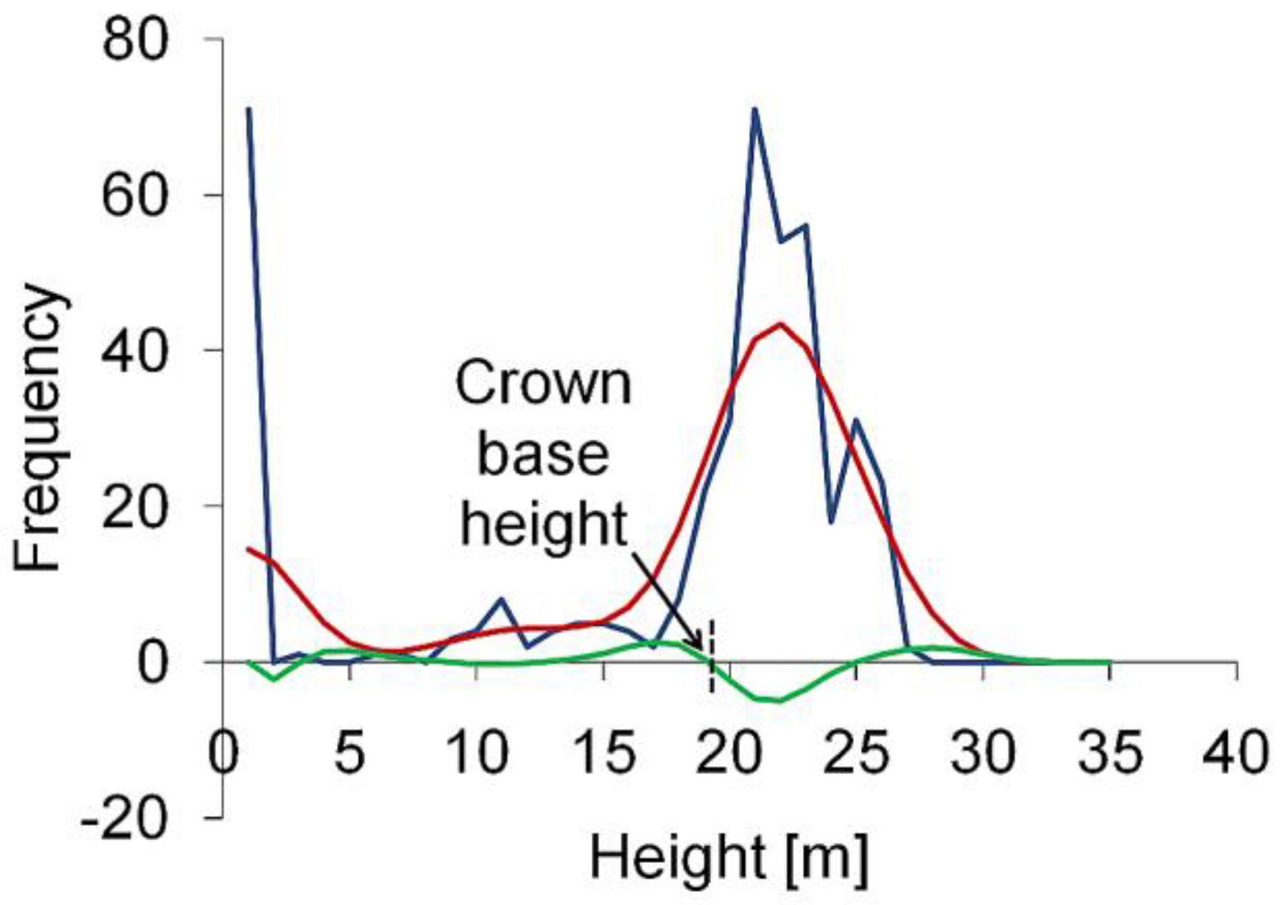
Nevertheless, it was possible to increase the strength of the relationship and to improve the estimation of stem volume with the crown diameter as an additional predictor. Model 5 with tree height and crown volume performed slightly worse which might be due to the fact, that the estimation of the crown base height from the ALS point cloud is not accurate enough. However, a denser point cloud might improve the identification of the crown base which has to be analysed in future studies. Moreover, the usage of all predictors (model 7) did not reduce the RMSE. In addition model 7 (and also 6) show a non-significant coefficient for cv which indicates once more that this variable does not contribute much to the models.

The RMSE of this study is in the range of the errors in most other studies carried out in Germany and Scandinavia. A selection of results is given in Table 11. However, a direct comparison is not possible due to different study sites with different forest stands and remote sensing data in addition to different validation techniques. A lower RMSE was reported by [10] for Norway spruce (Picea abies) and Fir (Abies alba) (RMSE = 16–17%). However, the prediction accuracy in this study is very close to the result of [22] who estimated the stem volume of Norway spruce (Picea abies L. Karst.), Scots pine (Pinus sylvestris L.) and birch (Betula spp.) with an RMSE of 22%.

Table 11. Selection of earlier studies carried out in Germany and Scandinavia to estimate individual tree stem volume from remote sensing features.

Study	Country	Species	RMSE
[33]	Southern Finland	Scots Pine (Pinus sylvestris), Norway spruce (Picea abies), Birch (Betula spp.)	31%
[10]	South-eastern Germany (Bavarian Forest National Park)	Norway spruce (Picea abies), Fir (Abies alba), European beech (Fagus sylvatica), Sycamore maple (Acer pseudoplatanus), Norway maple (acer platanoides), lime tree (Tilia europaea)	16–17% (coniferous trees) 29–32% (deciduous trees)
[11]	South-eastern Germany (Bavarian Forest National Park)		27% (coniferous trees) 35% (deciduous trees)
[22]	Southern Sweden	Norway spruce (Picea abies L. Karst.), Scots pine (Pinus sylvestris L.) and birch (Betula spp.)	22%

Table 11. Selection of earlier studies carried out in Germany and Scandinavia to estimate individual tree stem volume from remote sensing features.

Study	Country	Species	RMSE
[33]	Southern Finland	Scots Pine (Pinus sylvestris), Norway spruce (Picea abies), Birch (Betula spp.)	31%
[10]	South-eastern Germany (Bavarian Forest National Park)	Norway spruce (Picea abies), Fir (Abies alba), European beech (Fagus sylvatica), Sycamore maple (Acer pseudoplatanus), Norway maple (acer platanoides), lime tree (Tilia europaea)	16–17% (coniferous trees) 29–32% (deciduous trees)
[11]	South-eastern Germany (Bavarian Forest National Park)		27% (coniferous trees) 35% (deciduous trees)
[22]	Southern Sweden	Norway spruce (Picea abies L. Karst.), Scots pine (Pinus sylvestris L.) and birch (Betula spp.)	22%

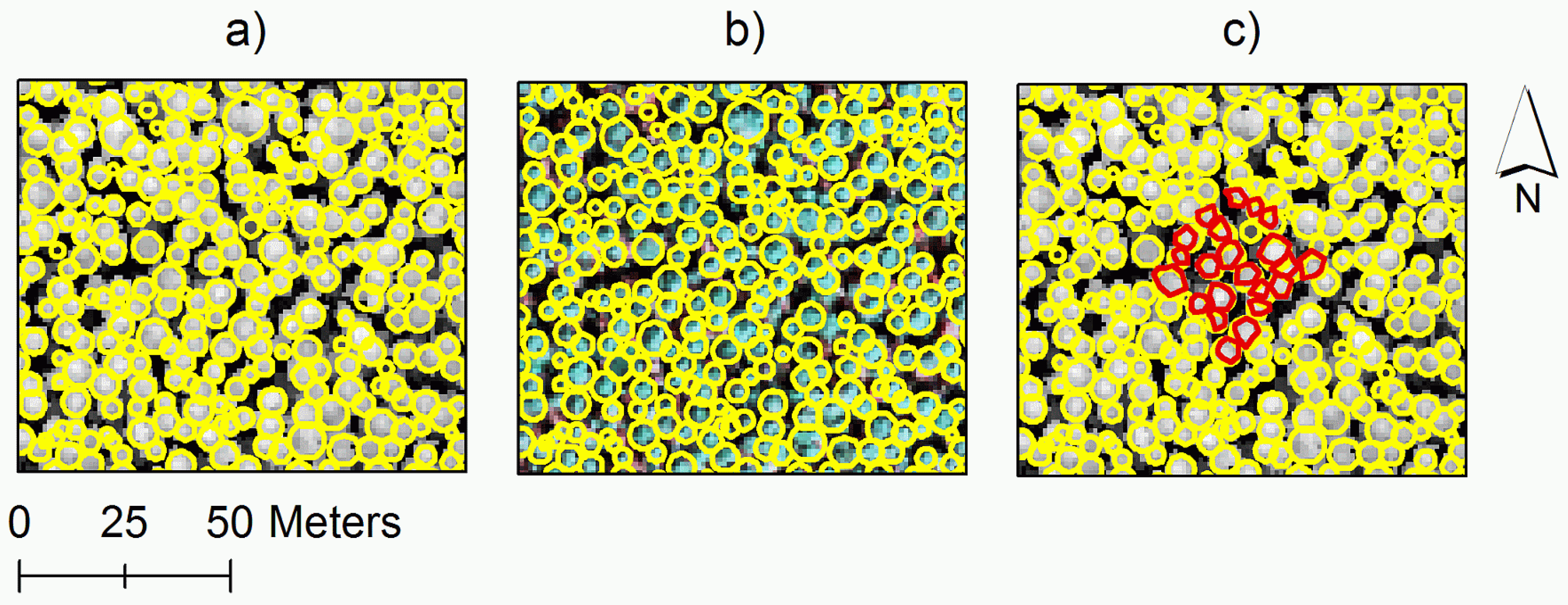
It was possible to delineate pine trees with an overall identification rate of ~62%. Compared to other studies this result is quite satisfying: In [13], 40−50% coniferous trees (mainly spruces) were delineated correctly in a study site in Austria. In [11], an identification rate of 38.7−45.4% was reported for both coniferous and deciduous trees in the Bavarian Forest National Park also using DSM based segmentation algorithms. As expected the detection of trees is much worse in young forest stands (age class II with a tree age ≤ 40 years) and very good for plots with an age class ≥ III with 86% correctly segmented trees. A DSM based segmentation technique was used in this study even though it is not possible to identify trees in lower canopy layers. It was assumed that a DSM based segmentation would be more robust compared to a tree extraction based on the ALS point cloud as suggested by others (e.g., [7]). Nevertheless in future studies the results should be compared to other delineation techniques.

In conclusion, it was possible to develop allometric models which can be used for stem volume estimation of pine trees based on features derived from airborne laser scanner and multispectral line scanner data. The automatic delineation of tree crowns was very successful in forest stands with an age class ≥ III. More research is definitely needed for dense deciduous forests in the temperate climate zones where the automatic segmentation of trees is frequently not accurate enough for the estimation of individual-tree-based information. Theoretically, a more sophisticated classification of different species might improve the discrimination of trees. Furthermore, models for the estimation of other quantitative tree attributes e.g., DBH and basal area have to be developed.

References and Notes

1. Hyyppä, J.; Hyyppä, H.; Yu, X.; Kaartinen, H.; Kukko, A.; Holopainen, M. Forest inventory using small-footprint airborne LiDAR. In Topographic Laser Ranging and Scanning, Principles and Processing; Shan, J., Toth, C.K., Eds.; CRC Press: Boca Raton, FL, USA, 2009; pp. 335–370. [Google Scholar]
2. Nothdurft, A.; Saborowski, J.; Breidenbach, J. Spatial prediction of forest stand variables. Eur. J. Forest Res. 2009, 128, 241–251. [Google Scholar] [CrossRef]
3. Straub, C.; Weinacker, H.; Koch, B. A comparison of different methods for forest resource estimation using information from airborne laser scanning and CIR orthophotos. Eur. J. Forest Res. 2009, 129, 1069–1080. [Google Scholar] [CrossRef]
4. Hollaus, M.; Wagner, W.; Schadauer, K.; Maier, B.; Gabler , K. Growing stock estimation for alpine forests in Austria: a robust lidar-based approach. Can. J. Forest Res. 2009, 39, 1387–1400. [Google Scholar] [CrossRef]
5. Breidenbach, J.; Kublin, E.; Mc Gaughey, R.J.; Andersen, H.E.; Reutebuch, S.E. Mixed-effects models for estimating stand volume by means of small footprint airborne laser scanner data. Photogramm. J. Fin. 2008, 21, 4–15. [Google Scholar]
6. Koch, B.; Heyder, U.; Weinacker, H. Detection of individual tree crowns in airborne lidar data. Photogramm. Eng. Remote Sensing 2006, 72, 357–363. [Google Scholar] [CrossRef]
7. Wang, Y.; Weinacker, H.; Koch, B. A lidar point cloud based procedure for vertical canopy structure analysis and 3D single tree modelling in forest. Sensors 2008, 8, 3938–3951. [Google Scholar] [CrossRef]
8. Reitberger, J.; Krzystek, P.; Stilla, U. 3D Segmentation and Classification of Single Trees with Full-Waveform LIDAR Data. In Proceedings of SilviLaser 2008, Edinburgh, UK, 17–19 September 2008; pp. 216–225.
9. Hollaus, M.; Mücke, W.; Höfle, B.; Dorigo, W.; Pfeifer, N.; Wagner, W.; Bauerhansl, C.; Regner, B. Tree Species Classification Based on Full-Waveform Airborne Laser Scanning Data. In Proceedings of Silvilaser 2009, College Station, TX, USA, 14–16 October 2009; pp. 54–62.
10. Reitberger, J.; Heurich, M.; Krzystek, P. Estimation of Stem Volume by Using 3D Segments Derived from Full-Waveform LiDAR Data. In Proceedings of SilviLaser 2010, Freiburg, Germany, 14–17 September 2010.
11. Heurich, M. Evaluierung und Entwicklung von Methoden zur automatisierten Erfassung von Waldstrukturen aus Daten flugzeuggetragener Fernerkundungssensoren. Ph.D. Dissertation, Technical University of Munich, Munich, Germany, 2006. [Google Scholar]
12. Heurich, M.; Weinacker, H. Automated tree detection and measurement in temperate forests of central europe using laserscanning data. In International Archives of the Photogrammetry, Remote Sensing and Spatial Information Sciences; ISPRS: Vienna, Austria, 2004; Volume 36, Part 8/W2; pp. 198–203. [Google Scholar]
13. Hyyppä, J.; Schardt, M.; Haggrén, H.; Koch, B.; Lohr, U.; Scherrer, H.U.; Paananen, R.; Luukkonen, H.; Ziegler, M.; Hyyppä, H.; Pyysalo, U.; Friedländer, H.; Uuttera, J.; Wagner, S.; Inkinen, M.; Wimmer, A.; Kukko, A.; Ahokas, E.; Karjalainen, M. HIGH-SCAN: The first european-wide attempt to derive single tree information from laserscanner data. Photogramm. J. Finl. 2001, 17, 58–68. [Google Scholar]
14. Breidenbach, J.; Gläser, C.; Schmidt, M. Diameter Distribution Modelling Using ALS. In Proceedings of SilviLaser 2008, Edinburgh, UK, 17–19 September 2008; pp. 266–273.
15. Hollaus, M.; Schadauer, K.; Dorigo, W. Kommt der gläserne Wald? Forstzeitung 2008, 2, 4–5. [Google Scholar]
16. Pflug, M.; Rindle, P.; Katzenbeisser, R. True-Ortho-Bilder mit Laser-Scanning und multispektralem Zeilenscanner. Photogrammetrie, Fernerkundung, Geoinformation 2004, 3, 172–178. [Google Scholar]
17. Weinacker, H.; Koch, B.; Heyder, U.; Weinacker, R. Development of filtering, segmentation and modelling modules for LIDAR and multispectral data as a fundamental of an automatic forest inventory system. In International Archives of the Photogrammetry, Remote Sensing and Spatial Information Sciences; ISPRS: Vienna, Austria, 2004; Volume 36, Part 8/W2; pp. 50–55. [Google Scholar]
18. Elmqvist, M.; Jungert, E.; Lantz, F.; Persson, Å.; Söderman, U. Terrain modelling and analysis using laser scanner data. In International Archives of the Photogrammetry, Remote Sensing and Spatial Information Sciences; ISPRS: Vienna, Austria, 2001; Volume 34, Part 3/W4; pp. 219–226. [Google Scholar]
19. FVA. Das Sorten- und Volumenprogramm BDAT. Availabe online: http://www.fva-bw.de/indexjs.html?http://www.fva-bw.de/forschung/bui/bdat.html (accessed on 03 January 2011).
20. Straub, C.; Dees, M.; Weinacker, H.; Koch, B. Using airborne laser scanner data and CIR orthophotos to estimate the stem volume of forest stands. Photogrammetrie, Fernerkundung, Geoinformation 2009, 3, 277–287. [Google Scholar] [CrossRef] [PubMed]
21. Hyyppä, J.; Inkinen, M. Detecting and estimating attributes for single trees using laser scanner. Photogramm. J. Fin. 1999, 16, 27–42. [Google Scholar]
22. Persson, Å.; Holmgren, J.; Södermann, U. Detecting and measuring individual trees using an airborne laser scanner. Photogramm. Eng. Remote Sensing 2002, 68, 925–932. [Google Scholar]
23. Solberg, S.; Næsset, E.; Bollandsas, O.M. Single tree segmentation using airborne laser scanner data in a structurally heterogeneous spruce forest. Photogramm. Eng. Remote Sensing 2006, 72, 1369–1378. [Google Scholar] [CrossRef]
24. MVTec. Pouring (Operator)—Segment an image by “pouring water” over it. In HALCON Reference Manual 10.0; MVTec Software GmbH: Munich, Germany, 2011; Available online: http://www.halcon.de/download/documentation/reference-10/pouring.html (accessed on 13 March 2011).
25. Hildebrandt, G. Fernerkundung und Luftbildmessung; Wichmann: Heidelberg, Germany, 1996. [Google Scholar]
26. Huss, J. Luftbildmessung und Fernerkundung in der Forstwirtschaft; Herbert Wichmann: Karlsruhe, Germany, 1984. [Google Scholar]
27. Næsset, E. Predicting forest stand characteristics with airborne scanning laser using a practical two-stage procedure and field data. Remote Sens. Environ. 2002, 80, 88–99. [Google Scholar] [CrossRef]
28. Næsset, E. Practical large-scale forest stand inventory using a small-footprint airborne scanning laser. Scand. J. Forest Res. 2004, 19, 164–179. [Google Scholar] [CrossRef]
29. West, P.W. Tree and Forest Measurement; Springer: Berlin/Heidelberg, Germany, 2003; pp. 39–44. [Google Scholar]
30. Husch, B.; Beers, T.W.; Kershaw, J.A. Forest Mensuration, 4th ed.; John Wiley & Sons, Inc.: Hobokon, NJ, USA, 2003; pp. 141–143. [Google Scholar]
31. Philip, M.S. Measuring Trees and Forests; CAB International: Wallingford, UK, 1994; pp. 74–78. [Google Scholar]
32. Chen, Q.; Gong, P.; Baldocchi, D.; Tian, Y.Q. Estimating basal area and stem volume for individual trees from lidar data. Photogramm. Eng. Remote Sensing 2007, 73, 1355–1365. [Google Scholar] [CrossRef]
33. Vauhkonen, J.; Korpela, I.; Maltamo, M.; Tokola, T. Imputation of single-tree attributes using airborne laser scanning-based height, intensity, and alpha shape metrics. Remote Sens. Environ. 2009, 114, 1263–1276. [Google Scholar] [CrossRef]