Article

Photorealistic Building Reconstruction from Mobile Laser Scanning Data

Finnish Geodetic Institute, P.O. Box 15, FI-02431 Masala, Finland
*
Author to whom correspondence should be addressed.
Remote Sens. 2011, 3(7), 1406-1426; https://0-doi-org.brum.beds.ac.uk/10.3390/rs3071406
Submission received: 28 April 2011 / Revised: 17 June 2011 / Accepted: 26 June 2011 / Published: 6 July 2011

Abstract

:
Nowadays, advanced real-time visualization for location-based applications, such as vehicle navigation or mobile phone navigation, requires large scale 3D reconstruction of street scenes. This paper presents methods for generating photorealistic 3D city models from raw mobile laser scanning data, which only contain georeferenced XYZ coordinates of points, to enable the use of photorealistic models in a mobile phone for personal navigation. The main focus is on the automated processing algorithms for noise point filtering, ground and building point classification, detection of planar surfaces, and on the key points (e.g., corners) of building derivation. The test site is located in the Tapiola area, Espoo, Finland. It is an area of commercial buildings, including shopping centers, banks, government agencies, bookstores, and high-rise residential buildings, with the tallest building being 45 m in height. Buildings were extracted by comparing the overlaps of X and Y coordinates of the point clouds between the cutoff-boxes at different and transforming the top-view of the point clouds of each overlap into a binary image and applying standard image processing technology to remove the non-building points, and finally transforming this image back into point clouds. The purpose for using points from cutoff-boxes instead of all points for building detection is to reduce the influence of tree points close to the building facades on building extraction. This method can also be extended to transform point clouds in different views into binary images for various other object extractions. In order to ensure the building geometry completeness, manual check and correction are needed after the key points of building derivation by automated algorithms. As our goal is to obtain photorealistic 3D models for walk-through views, terrestrial images were captured and used for texturing building facades. Currently, fully automatic generation of high quality 3D models is still challenging due to occlusions in both the laser and image data and due to significant illumination changes between the images. Especially when the scene contains both trees and vehicles, fully automated methods cannot achieve satisfactory visual appearance. In our approach, we employed the existing software for texture preparation and mapping.

Graphical Abstract

1. Introduction

The past few years have seen remarkable development in mobile laser scanning (MLS) to accommodate the need for large area and high-resolution 3D data acquisition. MLS serves one of the probably fastest growing market segments, which is 3D city modeling [1]. Advanced real-time visualization for location-based systems such as vehicle navigation [2] and mobile phone navigation [3] require large scale 3D reconstructions of street scenes. “Future developments in navigation and other location-enabled solutions will rely heavily on 3D mapping capabilities,” said Cliff Fox, executive vice president, NAVTEQ Maps, in November 2010 [4]. Google, Microsoft, Tele Atlas and NAVTEQ are currently expanding their products from 2D to 3D, even though currently most of their 3D models are only available for fly-through views. This has created a demand for ground-based models as the next logical step to offer 3D visualizations of cities [5]. The advantages of MLS data for high resolution 3D city models are obvious: MLS provides fast, efficient, and cost-effective data collection [6]. 3D models obtained from MLS offer high resolution visualization from walk-through views. However, the models with detailed building facades cannot be achieved from airborne laser scanning (ALS) and/or aerial images.
Typical data for 3D modeling come from airborne data, such as ALS and aerial images, and from terrestrial sources, such as terrestrial laser scanning (TLS), MLS, terrestrial images, and image sequences. Additionally building footprints/ground plans can assist when 3D models are created. In the following, a short review of both data types is presented.
In the past, photogrammetry has played a major role in the derivation of geographic data. However, despite significant research effort invested in developing automatic methods of data processing, the current level of automation is still low [7]. Following the development of electro-optical sensor technology together with the development of direct geo-referencing methods, since the mid-1990s, airborne laser scanning integrated with GPS and IMU has been available [8] for direct 3D data acquisition. The phenomenal development covering almost two decades has resulted in the current situation where the LIDAR system has become an important source of high resolution and accurate 3D geographic data [1]. As regards building reconstruction from airborne-based data, including ALS and images, reviews of reconstruction methods are included in publications such as those by Baltsavias [9], Brenner [7], Kaartinen and Hyyppä [10], and Haala and Kada [11]. Baltsavias [9] has mainly focused on knowledge-based methods for building extraction from aerial images. Brenner [7] has investigated reconstruction approaches based on different automated levels, in which the data were provided by airborne systems, whereas Kaartinen and Hyyppä [10] collected building extraction methods from eleven research agencies with four testing areas. Input data contain airborne-based data and ground plans (for selected buildings). Building extraction methods were analyzed and evaluated from the aspects of the time consumed, the level of automation, the level of detail, the geometric accuracy, the total relative building area and shape dissimilarity. Haala and Kada [11] reviewed building reconstruction approaches according to building structures: building roofs and building facades, in which the input data covered both airborne-based and ground-based data.
Data from TLS and close-range images are used only for small area modeling due to the slowness of acquisition and manual registration. Their main application focus is on the digital documentation of archaeological objects and architectural structures modeling [12]. A review of terrestrial image-based 3D modeling has been presented by Remondino [12]. According to Remondino [12], the methods for 3D information recovery from 2D images include the following: mathematical model transformation (e.g., photogrammetry), shape-based methods such as shape from shading, silhouette, 2D edge gradients, textures, specularity, and contour. However, automated image-based modeling methods for mobile system require highly-structured images with good texture, high frame rates, and uniform camera motion. Becker and Haala [13] proposed an approach for automated feature extraction for facade reconstruction by integrating TLS and terrestrial images in which the intensity values from TLS are used for the generating the reflectivity images, and then the corresponding relationships between reflectivity images and the green channel of terrestrial images are registered. The edges were extracted by means of the Sobel operation from terrestrial images. However, this method depends heavily on the intensity values from the scanner. Registration can fail if the intensity value is low. As is known, the wavelength of the scanner has some effect on how the intensity values correspond with RGB images. If IR wavelengths are used laser data is closer to IR images. Therefore, this method is not flexible.
For large-area modeling, MLS and image sequences are more efficient means of data collection. The camera-based mobile system is such that cameras with different views are mounted on a vehicle, integrated with GPS, and IMU data were used for high-resolution data collection. Based on these systems, automated building reconstruction methods have been proposed using image video sequences; e.g., Cornelis et al. [2], Pollefeys et al. [5], Tian et al. [14]. Pollefeys et al. [5] have presented an approach enabling detailed real-time 3D reconstruction from video streams. The video streams are collected by a multi-camera system (8 cameras) in conjunction with INS/GPS measurement. Model reconstruction from this system involves high computational costs due to large data redundancy (each surface element is typically seen via dozens of views). In addition, difficulties arise with large variability of illumination and varying distance and orientation of the observed scene. The resulting models are not geo-registered as GPS/INS was not fused with the results of vision-based pose estimation. In contrast, the data collected by MLS are location-based and more reliable and accurate, e.g., data collected with an accuracy of few centimeters.
Zhao et al. [15] have proposed a fully-automated method for reconstructing a textured CAD model of an urban environment using a vehicle-based system equipped with one single-row laser scanner and six line cameras plus a GPS/INS/Odometer-based navigation system. The laser points were classified into buildings, ground and trees by segmenting each range scan line into line segments and then grouping the points hierarchically. The vertical building surfaces were extracted by using Z-images, which were generated by projecting a point cloud onto a horizontal (X-Y) plane, where the value of each pixel in the Z-image is the number of the point cloud falling onto the pixel. However, for one building, the Z-image is not continuous in intensity due to the windows in the walls. Therefore, this method is not so useful when dealing buildings with large reflective areas, e.g., balconies with glass or windows. Additionally, problems related to object occlusion have been reported.
Früh et al. [16] introduced automated algorithms for generating textured facade meshes of cities using a truck equipped with one camera and two 2D laser scanners. The purpose of this method was to resolve object occlusions. A 2.5D depth image was employed to classify objects into foreground layers (occluded objects, e.g., trees) and background layers (e.g., building facades). This 2.5D depth image was obtained by regularizing 3D scan points into grids with each pixel representing the depth of the scan point. The grid position only specifies the topological order of the depth pixels, and not the exact 3D point coordinates. Large holes in the background layer, caused by occlusion due to the foreground layer objects, were filled in by interpolation. However, most of the operations that were performed on the depth image can be done just as well directly on the 3D point grid, but not as conveniently.
Our objectives are to reconstruct high-quality (mainly for visual quality) and high-accuracy (including model completeness and position accuracy) 3D models from mobile laser scanning data and terrestrial images. The past publications showed that even with fully-automated methods, it is still a challenging undertaking to achieve satisfactory visual appearance for the resulting models. Therefore, we propose a combination approach consisting of automated algorithms for geometry reconstruction, with additional manual checking and correction, and assisting software for texture preparation and mapping. Compact model size was required to enable the use of photorealistic models in a mobile phone for personal navigation.
This paper is organized as follows: Section 2 introduces our mobile laser scanning system and data acquisition for the Tapiola area. Building geometry reconstruction is addressed in Section 3. Section 4 illustrates texture preparation and mapping. The results and discussions are presented in Section 5, and Section 6 presents the conclusions.

2. Applied Data

The FGI ROAMER system is a mobile laser scanning system which can be mounted on various vehicles (see Figure 1). The hardware sub-systems of the ROAMER include the following: (1) a FARO laser scanner; (2) a GPS-INS navigation equipment; (3) a camera system; (4) synchronization electronics; and (5) a mechanical support structure. The current ROAMER MLS platform is constructed of hardened aluminum plates and profile tubes. The base plate is approximately 63 cm in length and width. The height of the scanner origin/mirror is approximately 97.5 cm above the base plate in the normal position when the scanner is in its upright position and between 36 cm and 57 cm when some of the tilted (fixed) positions are used. The possible negative tilt angles, or depression angles (DA), when the scanner’s z-axis points below the platform horizon are −60°, −45°, −30°, and −15°, whereas the positive tilt angles allow measurements at the angles of 0°, 15° and 30° above the platform horizon. The total weight of the intended instrumentation and the platform is approximately 40 kg [17].
The mirror rotation frequency, or profile measuring frequency of the FARO LS, is typically set to 24 Hz, 49 Hz or 61 Hz in mobile applications, and the vertical angular resolution can be set to 0.009–0.288 degrees (0.15–5.0 mrad, or 40,000–1,250 points per profile in the full FOV). The corresponding point spacing for adjacent points when using the typical scanning range of 15 m in road mapping is thus 2.2–75 mm along the scanning profile. For platform speeds of 50–60 km/h, the profile spacing is about 30 cm when using the profile measuring frequency of 49 Hz. With a frequency of 49 Hz, the profile interval is less than 20 cm when the speed of the mapping unit is kept below 40 km/h, and the point resolution along the profile is still 2.5–5 cm, which is sufficient for the practical ranges of 20–40 m, respectively, in the urban environment.
Figure 1. The FGI ROAMER system (photo from Kukko, A., 2009). Left: Side views of the platform design and instrumentation; Right: Image of the ROAMER (Here the scanner is tilted to the backward direction at a depression angle of 45°).
Remotesensing 03 01406 g001
The ROAMER configuration as used in Tapiola can be seen from Table 1. The data included altogether about 160,000 profiles, each profile having 2,150 points with 3D coordinates and return intensity, and 8,200 images. These profiles were divided into 162 files, each of them composed of around 1,000 profiles. Data collection lasted about one hour, and covered an area 180 m by 280 m. The laser data were transformed into map coordinate system (ETRS-TM35FIN with GRS80 ellipsoidal height).
Table 1. The ROAMER’s acquisition parameters.
Date12 May 2010
Laser scannerFaro Photon™ 120
Navigation systemNovAtel SPAN™
Laser point measuring frequency244 kHz
IMU frequency100 kHz
GPS frequency1 Hz
Data synchronizationSynchronizer by FGI, scanner as master
CamerasTwo AVT Pike
Profile measuring frequency49 Hz
Figure 2 shows the trajectory of data collection on top of an aerial image. It can be seen that the collected data contain all of the building facades in our test area. The data were collected during May, which is a time of the year when there is an abundance of leaves on the trees. Some of them are very close to the buildings (see images in Figure 2). Therefore, when developing algorithms, it is critical to consider how to separate buildings and trees. The algorithms for building geometry reconstruction are presented in the following section. Due to narrow streets and high buildings, images from the ROAMER system did not meet the requirement for high-quality textures. Therefore, the images were taken separately using a Canon EOS 400D digital camera.
Figure 2. The ROAMER trajectory and images from the Tapiola area (photo on the Left from Kaartinen, H., 2010).
Remotesensing 03 01406 g002

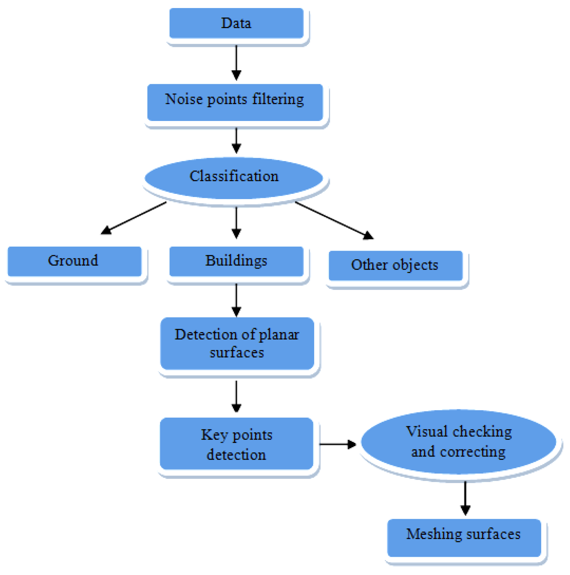
3. Geometry Reconstruction

The current situation is such that most of the existing commercial software for 3D model construction using laser scanner data primarily concentrates on using ALS data. Some software companies (e.g., Terrasolid) have developed tools for 3D modeling from both ALS and MLS data. The ALS data are for modeling building roofs and the MLS data are for modeling building facades. However, the huge dataset obtained when using the MLS option is challenging in large-area 3D model generation. Our goal in geometry reconstruction was to utilize some key points in building model construction. Figure 3 shows the procedure in geometry reconstruction. The detailed algorithms for noise point filtering, ground point classification, building point extraction, detection of planar surfaces, and derivation of the buildings’ key points are presented in each section.
Figure 3. The procedure applied in geometry reconstruction.
Remotesensing 03 01406 g003

3.1. Noise Point Filtering

The acquired data were composed of 162 files, totaling around 340 million points with XYZ coordinates. Noise point filtering was carried out individually on these 162 files. Each file contained noise points, object points, and ground points. There is no consistent definition for noise points in the literatures. In some papers, it is also called outlier points. In this paper, a noise point refers to a point with markedly deviation from the other points. Noise points are typical feature in point clouds produced with phase-based laser scanners. We used the data of 2D projections (xy, xz, yz) respectively to filter out these noise points. The data in each 2D projection were distributed into 10-by-1 bins. We used a three-dimensional histogram of bivariate data to calculate the number of elements falling into each bin of the grid, and we calculated the positions of each bin center. The threshold (T) for the number of the points in each bin can be defined by the user according to the different density of the point cloud and the size of a dataset. The detailed procedure can be seen from Figure 4. Figure 5 shows the filtering result from an example with a threshold (T) of 800 points.
Figure 4. The procedure in noise point filtering.
Remotesensing 03 01406 g004
Figure 5. An example of noise point filtering (YZ projection view). Left: Original data Right: Data after noise point removal. The figures are plotted in the same scale with the colors according to the height value of the points.
Remotesensing 03 01406 g005

3.2. Object Classification

The file sizes were greatly reduced following noise point removal. Consequently, the files were merged into groups of ten files, resulting in 16 groups. The last one was a group of 12 files. Each group contains around 6~10 million points. These files contained ground points, building points, tree points and other object points, which we wanted to separate.

3.2.1. Ground Point Classification

The data classification was performed file by file (16 files in total). The detailed procedure for one file is illustrated in the Algorithm 1. In order to facilitate the description, Table 2 depicts abbreviations used. This algorithm is performed in fully automation and is available for relatively flat area.
Table 2. A list of abbreviations.
AbbreviationDescription
Zf_dataThe most frequently occurring height value for data in one file;
Zf_gridThe most frequently occurring height value for data in each grid;
Z_minThe minimum height value for the data in one file;
Zmin_gridThe minimum height value for the data in the grid;
ZdThe difference between Zf_data and Zmin_grid
Algorithm 1 Ground point classification
1:   Calculate Zf_data: mode (height value of data)
2:   Compare the difference between Zf_data and Z_min
3:   if the difference <= 1m then
         points with the height value <= Zf_data +0.25m accepted as ground points
4:   else
          grid points in XY plane into 10*10 bins
5:       for each bin
               calculate Zf_grid and absolute value of Zd: abs(Zd)
6:          if abs(Zd) <= 3m then
                compare the difference between Zf_grid and Zmin_grid
8:             if the difference <= 0.25m then
                    points with the height value <= Zf_grid + 0.25 m as ground points
9:              else
                    points with the height value <= Zmin_grid + 0.25 m as ground points
10:            end if
11:         end if
12:     end for
13:     merge all ground points from each bin
14:  end if
This algorithm was developed by considering the most frequent occurring height value in the data. For the MLS data in the relatively flat area, ground points usually hold the most frequent occurring height value, especially in urban area without a large area of low vegetation. In this algorithm, the difference between Zf_data and Z_min was set to 1m. If the difference is less than 1m, it is considered as the terrain close to flat. We used 0.25 m as a tolerance taking into account the influence of measure accuracy of few decimeters in ROAMER system and also the unflatness of the terrain. In addition, a 3m threshold for Zd was used mainly considering that it is possible that data in some bins contain only the points from the reflection area due to the incomplete removal of the noise points. Figure 5 can also be an example in this case. However, for any algorithms, it is difficult to achieve perfect results. As can be seen, the noise point removal depended on the threshold value in each bin; what we can do is to take these factors into account and eliminate the effect. Figure 6 shows the result from the classification.
Figure 6. Ground point classification (from top view). Left: Ground points (yellow) and object points (green); Right: Ground points (yellow points).
Remotesensing 03 01406 g006

3.2.2. Building Point Classification

After ground point extraction, the remaining data contain buildings, trees and other objects. In 3D city model creation, building point classification is a key step in building model reconstruction. Unlike ALS data scanned from the several hundreds or even thousands of meters above the top of the objects, MLS data are collected close to the ground passing along a street. Detailed 3D information of the vertical planes of buildings can be obtained. The algorithms were developed based on the assumption that the building facades are vertical with respect to the ground. The method utilizes two different algorithms for building point classification according to the maximum height of the buildings in the dataset. For high buildings (buildings in the dataset with the maximum height greater than 20 m), Figure 7 shows the principle of this algorithm. We first utilize two cutoff boxes (cutoff box 1 and cutoff box 2) to find the overlap between them. They are the buildings of B1, B2, and B5. Here, I have to mention that after the overlap parts are detected, the whole buildings are extracted. Then these building points were removed from the data. The lower buildings were then extracted from the remaining data by setting two other cutoff boxes (cutoff box 3 and cutoff box 4). Then the overlaps between them can be found, which are B3, B4, B6, and B7. The benefit from this algorithm is that trees can then be effectively isolated from buildings, as in the most of cases tree points are not continuous in height. It means that from the top view, the shapes of trees from different cutoff boxes are different. Nevertheless, to deal with low buildings (buildings in the dataset with maximum height less than 20 m), we applied three cutoff boxes for building extraction. By deriving the overlaps between them, these points were merged and the duplicate points were deleted for rough building extraction. This part handled with the sparse points in the lower parts of the building to be collected from the scanner, e.g., due to parking places on the first floor of the building or columns in the lower part of the building. These occurred in the test data. Figure 8 shows the flow diagram of the algorithm. The detailed steps will be addressed in the following parts. In order to facilitate the description of the algorithm, Table 3 gives some short names instead of long description.
Figure 7. The basic principle of the algorithm of building point classification.
Remotesensing 03 01406 g007
Figure 8. The procedure in building point classification.
Remotesensing 03 01406 g008
Table 3. A list of name substitution.
NameDescription
Z_maxMaximum height value in the data (one file);
Z_minMinimum height value in the data (one file);
Z_midEquals to (Z_max+Z_min)/2-2m;
ZgThe average height of ground points;
(1)
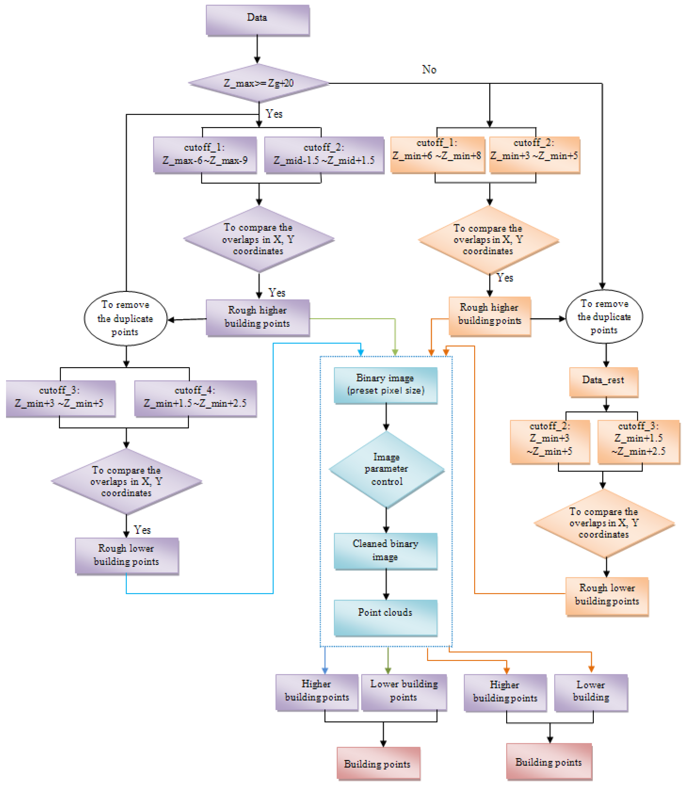
Algorithm for data in which the maximum height of the buildings is greater than 20 m.
(i)
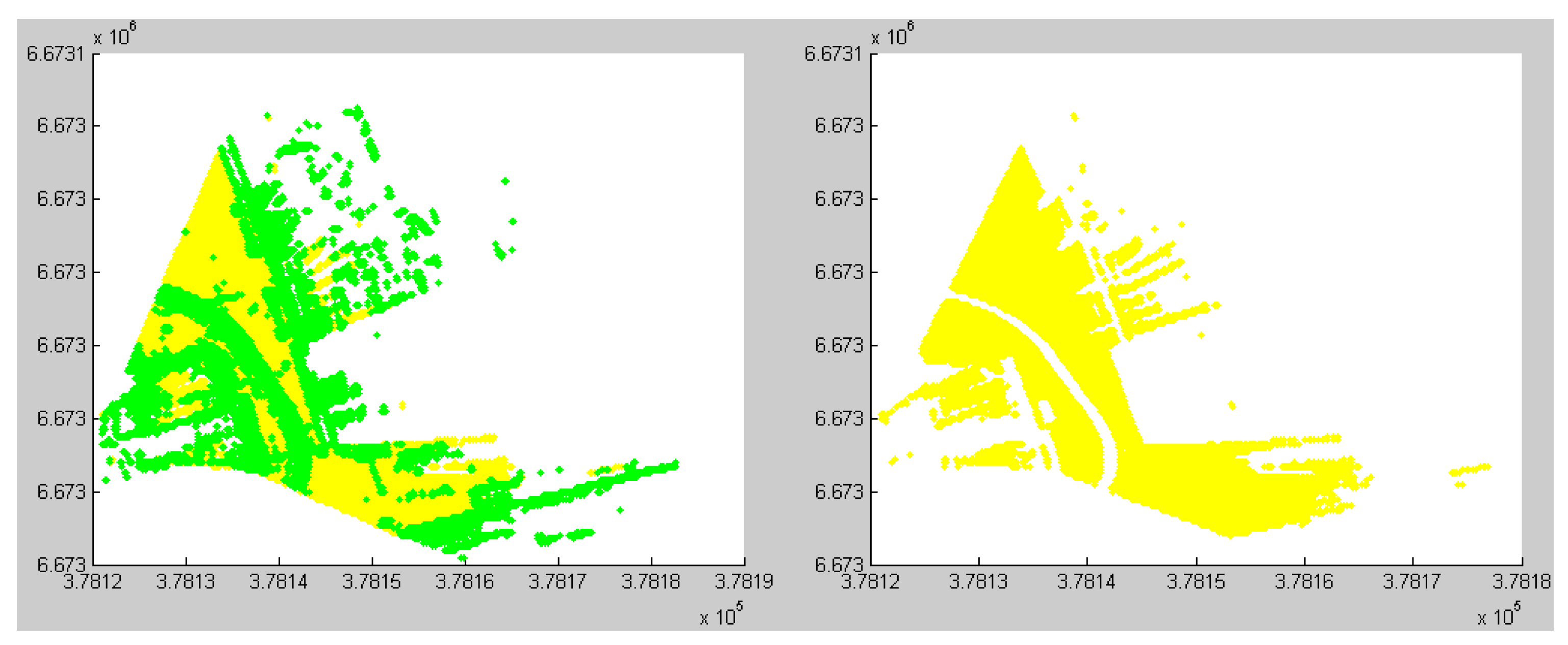
Roughly extract higher buildings by obtaining points from two cutoff boxes (cutoff_1 and cutoff_2) and comparing the X and Y coordinates of points between the boxes.
Firstly, two cutoff boxes are set to extract the points: cutoff_1: Z_max − 6 m~Z_max − 9 m; cutoff_2: Z_mid − 1.5 m~Z_mid + 1.5 m. The threshold for cutoff_1 is set mainly considering that on the top of some buildings, there are some prominent parts, for example, elevator tower, roof windows, and water tanks, which are the parts of the buildings, but these points cannot be used as parts of the continuous buildings. In some cases, noise points from the top of the buildings could not be completely removed (Figure 5). Therefore we start to obtain points from the setting threshold: Z_max − 6 m. For this threshold, it works whatever there exist prominent parts or noise points on the buildings or not. Due to the cutoff_1 starts from Z_max – 6 m, therefore the Z_mid is set to (Z_max+Z_min)/2 − 2 m. Since buildings are always continuous, the overlaps of the two sets of cutoff data in XY coordinates can be derived by:
  • TF1 = ismember (cutoff_2 (:, [x, y]), cutoff_1(:, [x, y]), ‘rows’);
  • Idx1 = find (TF1 == 1);
  • Part_highBuilding = cutoff_2 (Idx1, [x, y, z]);
  • TF2 = ismember (objectPoints (x,y), Part_highBuilding (x,y), ‘rows’);
  • Idx2 = find (TF2 == 1);
  • highBuilding = objectPoints (Idx2,[x, y, z]);
Thus, the higher buildings were extracted roughly. As a result, the whole building is extracted, not only a part of the building. However, in these data, there were still some other points besides building points, e.g., tree points. It will be further processed on the step (iii).
(ii)
Similarly, roughly extract lower buildings by obtaining points from two cutoff boxes (cutoff_3 and cutoff_4) and comparing the X and Y coordinates of points between two boxes.
After the higher buildings had been roughly extracted on the step (i), these points were removed from the data. Then we set two more cutoff boxes for detecting lower building. Cutoff_3: Z_min + 3 m~Z_min + 5 m; cutoff_4: Z_min + 1.5 m~Z_min + 2.5 m. As we know, the smaller the height of cutoff box, the less the number of the points in the box. The separation of building points from trees is easier. However, we have to consider that if there are windows in the cutoff area, it would lead to incomplete building extraction. For example, in one cutoff box, there are points on the wall and another cutoff box has less points or is even empty due to window reflection. After comparing the overlap between them, the result would lead to the missing of this building facade. Therefore, in order to avoid this context, the height of the cutoff boxes should be set properly. By applying the similar method as the step (i), overlaps of XY coordinates in the cutoff_3 and cutoff_4 datasets were obtained. Consequently, lower buildings were roughly extracted. But there were still other points included besides these building points. Therefore, further process will be performed on the step (iii).
(iii)
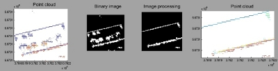
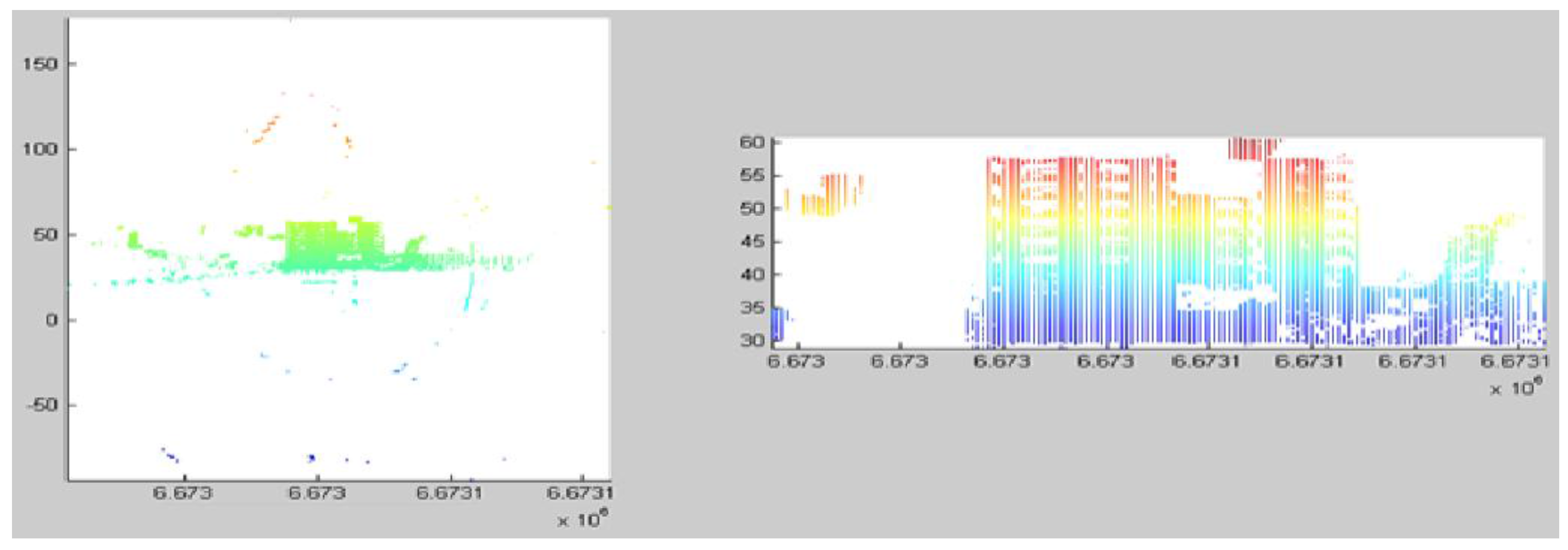
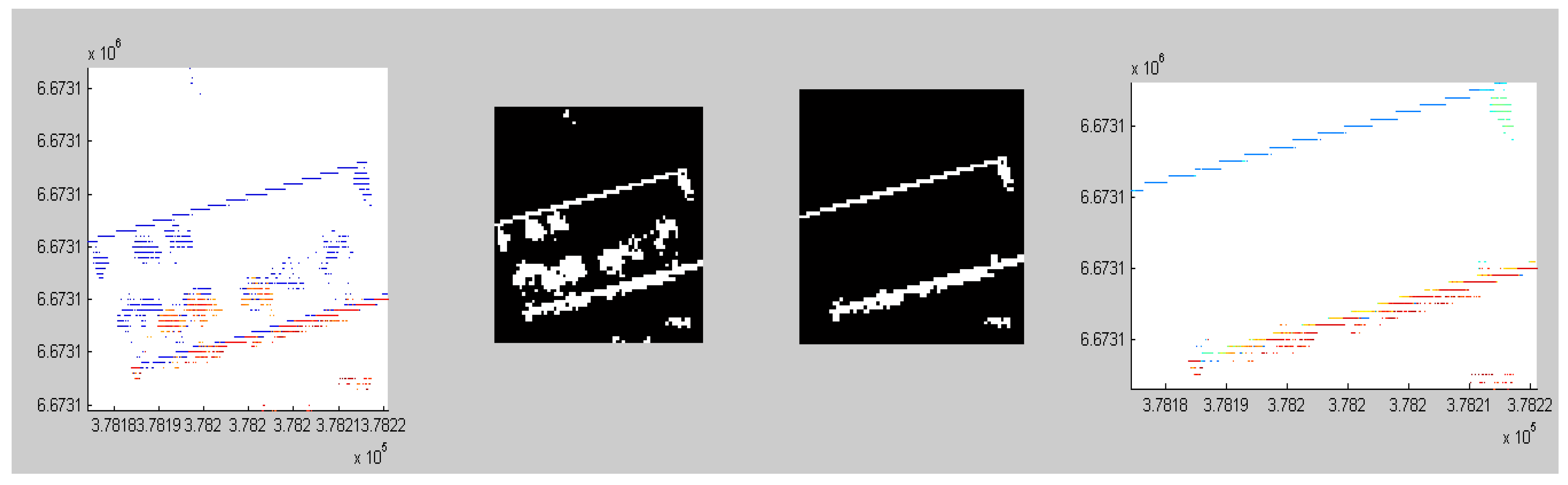
By transforming these roughly detected building points into binary images, image parameters could be set to remove the non-building points.
The purpose of this step was to remove non-building points by means of image processing technology. Firstly, the pixel size for binary image was predefined. Then we defined the size of the binary image from the XY coordinates of the extracted rough building points. A binary image could be formed by setting objects as 1 and empty as 0 from the roughly-detected building points from step (i) and (ii). In order to eliminate small and irregular areas (non-building areas) from the image, it is possible to set the thresholds for region properties, e.g., area size and eccentricity. For example, when the eccentricity value of an area is close to 1, it implies that the shape of the area is close to a line. When the eccentricity value is close to 0, the shape of the area is close to a circle. Usually, the shape is close to a line when a building facade is seen from the top, but a tree is close a circle (see Figure 9). For a square-like building, the eccentricity value can be set to a small value e.g., 0.3~0.5. However, it is possible that some tree points cannot be effectively separated. Thus, we can also utilize other parameters e.g., area size and other shape parameters (explain later on) to restrict it. Usually the MLS data are collected along the streets. Large dataset, in order to avoid sudden heavy computation or the situation of being out of memory, is processed usually by separating into several groups according to the number of profiles. Therefore, one group may contain only a part of a building e.g., one facade or two facades. Thus, the parameter ‘eccentricity’ can be effectively applied to these cases. As regards the shape of an area, besides the eccentricity, we can also use the region properties of major axis length and minor axis length to remove some irregular areas. An example of the pseudo codes:
  • LabeledImage = bwlabel (binaryImage, 8);
  • Stats = regionprops (LabeledImage, ‘Area’, ‘Eccentricity’, ‘MajorAxisLength’, ‘MinorAxisLength’);
  • Find objects with Stats.Area > 4m2 and Stats.Eccentricity = 0.8 and Stats.MajorAxisLength < 15 m and Stats.MinorAxisLength > 4 m.
As we have mentioned in the above, there were a lot of trees very close to the building facades. It is challenging work to separate and classify buildings from trees by only applying region properties. Therefore, we created a morphological line structuring element. A morphological structure element can be constructed by a specific shape such as a line or a disk. For a line structure element, the length of the line and the angle of the line as measured in a counterclockwise direction from the horizontal axis should be predefined. In our case, the angle of the line structure element was set approximately to the building edge direction e.g., 10°. The line structure element can be set as: se = strel (‘line’, the length of line, the direction of line). This enabled the adhesion parts between building edges and trees to be effectively separated.
(iv)
The processed binary image was transformed back into point cloud.
(v)
Applying steps (iii) and (iv) to the results derived from step (i) and step (ii), and merging the points, the buildings were finally extracted.
Figure 9. An example of the procedure of transformation of 3D point clouds into 2D binary images, non-building points filtering on images, then into 3D point clouds.
Remotesensing 03 01406 g009
(2)
Algorithm for data in which the maximum height of the buildings is less than 20 m.
(a)
Set three cutoff boxes: cutoff_1: Z_min + 6 m~Z_min + 8 m; cutoff_2: Z_min + 3 m~Z_min + 5 m; cutoff_3: Z_min + 1.5 m~Z_min + 2.5 m.
(b)
Derive the overlap points between cutoff_1 and cutoff_2 and remove the overlap points from the data:
  • P_overlap1= {P(x, y)   cutoff_1 & P(x, y)   cutoff_2 | P   all points};
  • P_1(x, y, z) = {P (x, y) ==P_overlap1(x, y) | P   all points};
  • Data_rest (x, y, z) = {~ (P_1 all points)}.
(c)
Derive the overlap points between cutoff_2 and cutoff_3 from ‘Data_rest’:
  • P_overlap2= {P(x, y)   cutoff_2 & P(x, y)   cutoff_3 | P   data_rest};
  • P_2(x, y, z) = {P (x, y) == P_overlap2(x, y) | P   Data_rest};
(d)
Apply step (iii) and step (iv) in the previous algorithm to P_1 and P_2 and merge the resulting building points.
We applied different algorithms for different datasets according to the maximum height value in the dataset. Except several parameters needed to be predefined, the algorithms are fully automatic. These predefined parameters include pixel size for binary image, image region properties: area size, eccentricity value, major axis length and minor axis length, and also morphological structure element. It is not a good option to use consistent parameters for all datasets. However, for region properties, except eccentricity value, other parameters can be applied for all datasets after setting. Morphological structure element is applied mainly for separating between building facade and trees. When the scene does not contain trees, this parameter is useless. For example, the length of structure element of line-shape is set to 1. Pixel size and eccentricity value are sensitive to the results. According to different dataset, these parameters should be set properly. Figure 10 shows an example how different pixel sizes affect the results. When pixel size is set to 0.5 m, small objects are independent. By the thresholds of area size and shape, these small objects are removed. In contrast, for image with pixel size of 1.5 m, objects are connected each other. After filtering, these objects are still preserved. However, large pixel size can cause more noise included. Therefore, when the scene shows discontinuous building points, good result can be obtained by applying large pixel size.
Figure 10. An example in the analysis of the sensitivity of the parameter (pixel size of binary image). Left: image with noise points; Middle: image after noise removal; Right: results in 3D points; Upper: images with pixel size of 0.5 m; Lower: images with pixel size of 1.5 m.
Remotesensing 03 01406 g010
Sixteen files were processed using the algorithms and building points were successfully extracted. In order to seamlessly continue the process, the building points were merged into four files. Each file contains around 9 million points. Figure 11 shows example results of classification of building points.
Figure 11. The results from building point classification (The colors show different heights).
Remotesensing 03 01406 g011

3.3. Key Point Extraction and Surface Meshes

One of our goals was to generate building models that require low amount of memory and can thus be applied for applications such as mobile devices with limited memory, and rapid rendering for visualization. The buildings extracted by applying the above steps still have a huge amount of points. Therefore, key point extraction was essential. We took two steps for key point extraction: to identify each building facade and to extract the key points.

3.3.1. Identifying Each Building Facade

In our test data, almost all buildings are rectangular with planar (non-curved) facades. Therefore, we can use the coplanar condition to identify a building facade. The algorithm is realized as follows:
(1)
Two neighbor points (P1, P2) were selected randomly to form a vector (V1).
(2)
A third point (P3) was added to form the vector V2 with P1. If V2 was not parallel to V1, then it was considered to be the basic plane.
(3)
If V2 and V1 were collinear, then this point (P3) was taken as a coplanar point. If not, then the next step was taken.
(4)
P4 is any point in the dataset. P4 and P2 formed vector V3. Does it satisfy the coplanar condition V3(V1 × V2) = 0? If yes, it is a coplanar point.
(5)
When a plane was identified, the points of this plane were removed from the dataset.
(6)
Steps (1) to (5) were repeated until all points were allocated to a certain plane (Figure 12).
Figure 12. Detection of coplanar point detection (different colors represent different planes).
Remotesensing 03 01406 g012

3.3.2. Key Point Extraction

The implementation of the above algorithm enabled each building plane to be identified. It is easy to obtain the corners of the plane from identified building plane as each plane was almost rectangle. The corners could be deduced from the minimum and maximum values of the X or Y coordinates and the Z values. However, sometimes the corner points based on laser data are not exactly where the corners of the buildings are. Therefore, small adjustments were necessary to ensure the rectangular building facades. For example, as regards the upper corners of one building facade, they usually had the same height values. And the upper corner and its corresponding lower corner had the same X, Y coordinates. In addition, manual checking and correction were important in order to achieve high quality (e.g., completeness and correctness) of building geometry. For example, in some building facades, due to object reflection (e.g., glass) or object occlusions (e.g., trees or other objects), it was possible for the points in building facades to be sparse and discontinuous. Manual checking and correction are performed by visually comparing the identified building planes and corners with terrestrial images and also making correction by resetting parameters in the algorithm for better results.
The advantage in our data is that the buildings are scanned from all sides. This means that complete models can be created with manual assistance. The disadvantage is that we have no ALS data for roof information. This means that more manual operation is needed.
Following key point extraction, the meshes were constructed for the surfaces. When dealing with complex buildings, they were divided into cubes according to different heights. The meshing surfaces were imported to 3ds Max for further operations, e.g., surface merging and small geometry adjustment for good visualization. Figure 13 shows the raw models produced using 3ds Max.
Figure 13. Raw models of Tapiola area produced using 3ds Max.
Remotesensing 03 01406 g013

4. Texture Preparation and 3D Mapping

A detailed procedure of geometry reconstruction from MLS data has been addressed in the above steps. Geometric models of buildings exclude societal information, e.g., landmarks, related to the real scene. Models with textures not only offer rich content to guide people’s life, e.g., personal navigation, but they also provide good visualization.
Due to narrow streets and high buildings, images from the ROAMER system did not meet the requirement for high-quality textures. Therefore, the images were taken separately using a Canon EOS 400D digital camera. These images were used to provide the textures of the building facades. For complete 3D models, the textures of the building roofs were also needed. We made use of aerial images from Bing Maps (http://www.bing.com/maps/) to obtain the textures of the building roofs. Each roof plane was made to correspond to one texture. Image processing software (Corel Photo Paint) was utilized in texture preparation, e.g., the image perspective correction, noise point removal, and image mosaicing. The 3ds Max software was used in texture mapping.

4.1. Texture Preparation

Textures were prepared from the images for individual building facades. Images taken in the field cannot be directly used for textures due to the following reasons:
(1)
Images were taken at a certain oblique angle to the building facades requiring perspective correction.
When objects obstruct the line of sight in front of a building or if buildings are high, the images have to be taken at an oblique angle. In addition, even if images were taken at approximately right angles to the building facade, they still need some perspective correction.
(2)
With large building facades, several images are needed for a single texture, and consequently image mosaicing was needed.
Due to the limited field of view of the camera when covering a large building facade, one image only covered part of the building facade. Thus, several images needed to be combined to create an image mosaic of the facade. The texture shown in Figure 14 is a mosaic of seven images from left to right; with high buildings, images needed to be combined from the upper part and the lower part.
(3)
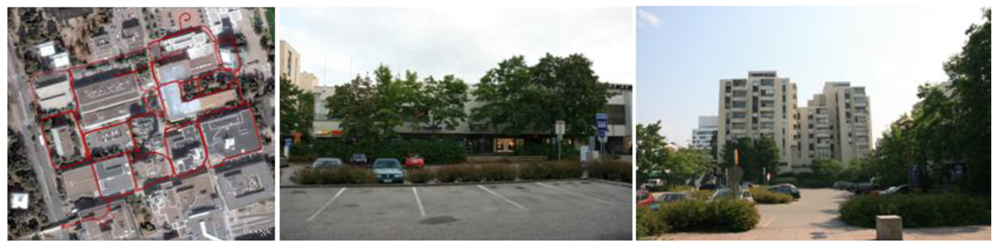
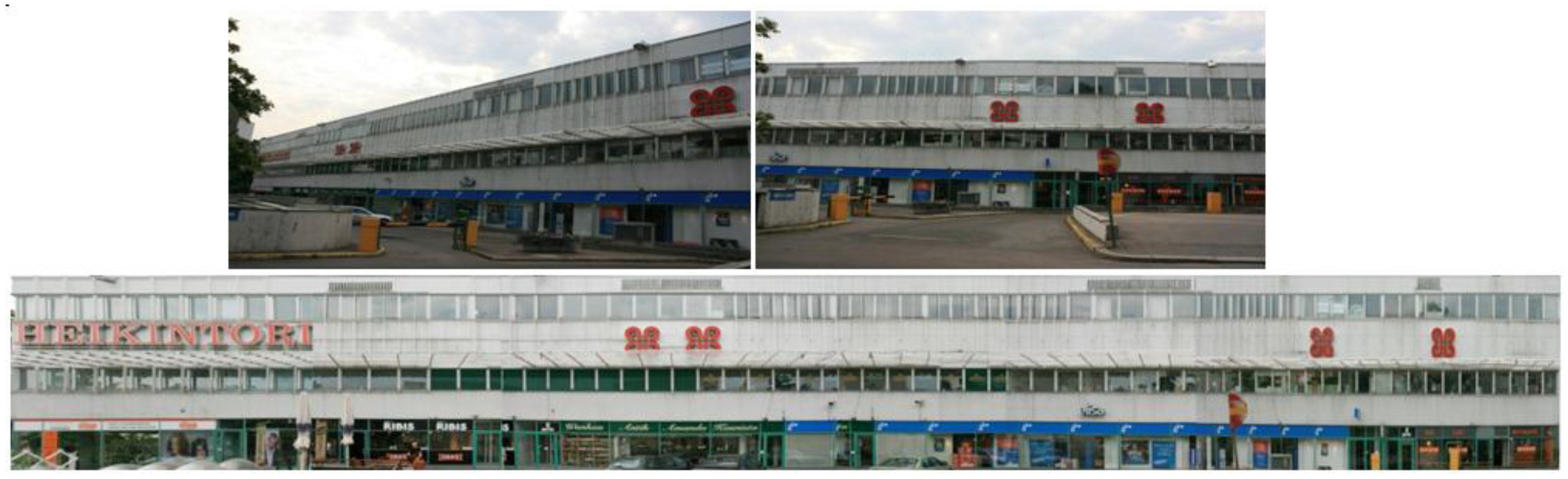
Due to some objects causing occlusions, e.g., trees close to buildings, there is noise, e.g., tree shadows, in the images of the building facades. This noise needs to be removed from the image.
In this test area, as mentioned above, there are a lot of trees. Some of them are very close to the building facades (see the middle image of Figure 2). In this context, tree shadows on the building facades needed to be removed from the images for the sake of the high quality texture. Figure 14 is an example showing the original images taken at a certain oblique angle due to some objects obstructing the direct line of sight to the building. The Figure 14 also shows the texture from multi-image mosaic. In addition, in the lower part of the first image of Figure 14, some noise was removed for the final texture (see the lower image of Figure 14).
Figure 14. Images and texture. Upper: Two images; Lower: Texture.
Remotesensing 03 01406 g014

4.2. Texture Mapping

Once the raw models and textures have been prepared, the textures need to be projected onto the building facades. This work was processed by means of the 3ds Max software. As is mentioned in the above, for the Tapiola models, each building facade or building roof was matched to each texture. This made the mapping process relatively easy. The UVW mapping method was employed in 3ds Max. UVW is a mapping process for transferring a 2D image onto 3D object surfaces. It applies mathematical functions to assign each point on the texture to each point on the object surface. Figure 15 shows the models after texture mapping.
Figure 15. Models with textures provided via 3ds Max.
Remotesensing 03 01406 g015

5. Results and Discussions

Using the automated methods presented here for geometry reconstruction and assisted by software for texture mapping, we reconstructed photorealistic 3D models of the Tapiola area (Figure 16). The results met our goals: the models were small in size due to only four corners representing one building facade; the accuracy of the models was adequate for personal navigation, and we achieved good visual appearance. Our models were tested on a mobile phone embodying a navigation application. Rapid rendering and continuous navigation were realized owing to the small size of the models. Despite GPS signal constraints in the urban area, the accuracy of the models met the outdoor navigation requirements (required within 1 m model accuracy). However, our approach for complete model reconstruction required both automated algorithms and manual operations. Therefore, the efficiency was relatively low. There are two factors which have a great impact on the efficiency of 3D model construction. One is the result obtained from the automated process, which affects the work load in manual correction. The other is the process of texture preparation.
(1)
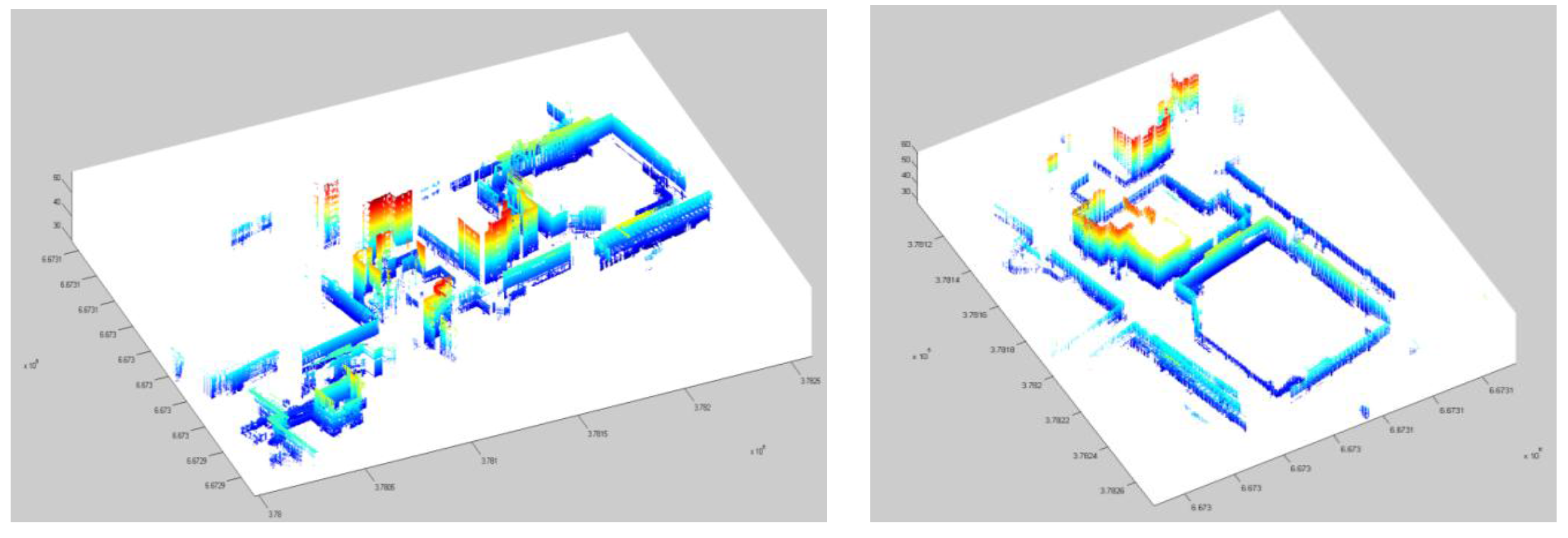
Automated process: We developed automated algorithms for noise point filtering, ground classification, building point classification, detection of planar surfaces, and building key point extraction. The result produced by building point classification had the greatest impact on the follow-up processes. Due to reflection from objects, the data from the laser scanner is subject to discontinuities. When some small area data were filtered out as noise points, it occasionally causes incompleteness of the building. In our method, we utilized binary images to clean the noise. The area and shape of an area were constrained to certain threshold values. Therefore, it was important to decide appropriate thresholds for non-building point filtering. The work load in manual checking and correction for model completeness depends on not only the quality of original data but also the results from the automated process.
(2)
The process of texture preparation. This step was processed manually. As the images were taken separately from the MLS system, there was no orientation information for automatic process. In addition, object occlusions on images, especially tree occlusions, resulted in the unpleasant appearance of building facades. This caused a lot of work in texture preparation.
Figure 16. 3D models of Tapiola.
Remotesensing 03 01406 g016
Fully automated 3D model generation was our common goal. However, the proposed fully-automated methods, e.g., from Zhao et al. [15] and Früh et al. [16], could not delivery satisfactory results, especially as regards visual appearance. The main reason was that there was no efficient way to resolve object occlusions. Besides this, there were other reasons affecting the results. For example, Früh et al. [16] proposed a fast and efficient way for 3D models, but the resulting models were characterized by their large data size due to surface meshes constructed from point clouds. The method presented by Zhao et al. [15] produced a model of limited accuracy due to a mismatch between the scanner and the cameras. Despite the satisfactory results achieved as we applied our approach, the level of automation was still low. This can be improved as follows:
(1)
By integrating with the ALS data.
The degree of building completeness can be considerably improved during the process of geometry reconstruction by integrating the MLS data with the ALS data. This will mean a reduced work load in manual correction. However, new problems would rise from data integrating due to different data sources. ALS and MLS provide data with different resolutions, and probably from different years. And different geometry matching would lead to accuracy lost.
(2)
By utilizing images from cameras mounted on the platform of our ROAMER system.
As regards building textures, we used cameras with wide fields of view and proper viewing angles from our ROAMER system, and synchronized time from GPS, IMU. The scanner and cameras can be used for identifying the corresponding relationships between point clouds and images so that automated texture mapping could be achieved by applying orientation information from images. Object occlusions on the images could be improved by employing images taken from different viewing angles or by detecting the location of windows on building facades from point clouds and applying consistent textures for the building walls.

6. Conclusions

3D models were successfully reconstructed from Mobile Laser Scanning data (MLS) and terrestrial images using automated algorithms for geometric reconstruction, interactive checking and correction for model completeness, and software assisting in texture preparation and mapping. Point data were acquired by using the ROAMER system developed at the Finnish Geodetic Institute (FGI). Models were reconstructed mainly in two steps: (1) geometry reconstruction, including fully-automated classification of building points, corner detection, and interactive checking for completeness of building geometry, and (2) photorealistic texture mapping. In Tapiola, our testing area, the scenes covered a number of trees and some were very close to the building facades, which was challenging when considering discriminating between buildings and trees. In this study we present detailed algorithms for noise point filtering, ground classification, building point classification, coplanar point detection and key points of model derivation. We used line structure elements to separate buildings and trees from binary images. The results showed realistic 3D scenes. Small model size, desired accuracy, and good visual appearance were achieved and the models were tested using a mobile phone for personal navigation. A satisfactory result was achieved.
Future work in this subject area will focus on improving the level of automation by integrating MLS data with ALS data, and by utilizing images from ROAMER system by applying cameras with proper fields of view and by adjusting their viewing angles with respect to the building facades.

Acknowledgements

The authors of this paper would like to thank Tekes for the financial support it has granted to the 3D-NAVI-EXPO project and the Academy of Finland for its support of the 3DGIS project.

References and Notes

  1. Toth, C. R&D of Mobile Mapping and Future Trends. In Proceedings of the ASPRS Annual Conference, Baltimore, MD, USA, 9–13 March 2009.
  2. Cornelis, N.; Leibe, B.; Cornelis, K.; Van Gool, L. 3D urban scene modeling integrating recognition and reconstruction. Int. J. Comput. Vis. 2008, 78, 121–141. [Google Scholar] [CrossRef]
  3. Chen, R.; Kuusniemi, H.; Hyyppä, J.; Zhang, J.; Takala, J.; Kuittinen, R.; Chen, Y.; Pei, L.; Liu, Z.; Zhu, L.; et al. Going 3D, Personal Nav and LBS. GPS World 2010, 21, 14–18. [Google Scholar]
  4. NAVTEQ Acquires PixelActive Acquisition Reinforces the Company’s Commitment to Leadership in 3D Mapping. 17 December 2010. Available online: http://corporate.navteq.com/webapps/NewsUserServlet?action=NewsDetail&newsId=946&lang=en&englishonly=false (accessed on 17 December 2010).
  5. Pollefeys, M.; Nister, D.; Frahm, J.M.; Akbarzadeh, A.; Mordohai, P.; Clipp, B.; Engels, C.; Gallup, D.; Kim, S.J.; Merrell, P.; et al. Detailed real-time urban 3D reconstruction from video. Int. J. Comput. Vis. 2008, 78, 143–167. [Google Scholar] [CrossRef]
  6. El-Sheimy, N. An overview of mobile mapping systems. In Proceedings of FIG Working Week 2005 and GSDI-8—From Pharaos to Geoinformatics, FIG/GSDI, Cairo, Egypt, 16–21 April 2005; p. 24.
  7. Brenner, C. Building reconstruction from images and laser scanning. Int. J. Appl. Earth Obs. Geoinf. 2005, 6, 187–198. [Google Scholar] [CrossRef]
  8. Petrie, G. An introduction to the technology, mobile mapping systems. Geoinformatics 2010, 13, 32–43. [Google Scholar]
  9. Baltsavias, E.P. Object extraction and revision by image analysis using existing geodata and knowledge: Current status and steps towards operational systems. ISPRS J. Photogramm. Remote Sens. 2004, 58, 129–151. [Google Scholar] [CrossRef]
  10. Kaartinen, H.; Hyyppä, J. EuroSDR-Project Commission 3 “Evaluation of Building Extraction”. Final Report; In EuroSDR: European Spatial Data Research, Official Publication; EuroSDR: Dublin, Ireland, 2006; Volume 50, pp. 9–77. [Google Scholar]
  11. Haala, N.; Kada, M. An update on automatic 3D building reconstruction. ISPRS J. Photogramm. Remote Sens. 2010, 65, 570–580. [Google Scholar] [CrossRef]
  12. Remondino, F.; El-Hakim, S. Image-based 3D modelling: A review. Photogramm. Rec. 2006, 21, 269–291. [Google Scholar] [CrossRef]
  13. Becker, S.; Haala, N. Combined Feature Extraction for Facade Reconstruction. In Proceedings of the ISPRS Workshop Laser Scanning 2007 and SilviLaser 2007, Espoo, Finland, 12–14 September 2007; pp. 241–247.
  14. Tian, Y.; Gerke, M.; Vosselman, G.; Zhu, Q. Knowledge-based building reconstruction from terrestrial video sequences. ISPRS J. Photogramm. Remote Sens. 2010, 65, 395–408. [Google Scholar] [CrossRef]
  15. Zhao, H.; Shibasaki, R. Reconstructing a textured CAD model of an urban environment using vehicle-borne laser range scanners and line cameras. Mach. Vis. Appl. 2003, 14, 35–41. [Google Scholar] [CrossRef]
  16. Früh, C.; Zakhor, A. An automated method for large-scale, ground-based city model acquisition. Int. J. Comput. Vis. 2004, 60, 5–24. [Google Scholar] [CrossRef]
  17. Kukko, A. Road Environment Mapper—3D Data Capturing with Mobile Mapping. Licentiate’s Thesis, Helsinki University of Technology, Espoo, Finland, 2009; p. 158. [Google Scholar]

