Segment-Based Land Cover Mapping of a Suburban Area—Comparison of High-Resolution Remotely Sensed Datasets Using Classification Trees and Test Field Points

Abstract

In order to better understand and exploit the rich information content of new remotely sensed datasets, there is a need for comparative land cover classification studies. In this study, the automatic classification of a suburban area was investigated by using (1) digital aerial image data; (2) digital aerial image data and laser scanner data; (3) a high-resolution optical QuickBird satellite image; (4) high-resolution airborne synthetic aperture radar (SAR) data; and (5) SAR data and laser scanner data. A segment-based approach was applied. The classification rules for distinguishing buildings, trees, vegetated ground, and non-vegetated ground were created automatically by using permanent test field points in a training area and the classification tree method. The accuracy of the results was evaluated by using test field points in validation areas. The highest overall accuracies were obtained when laser scanner data were used to separate high and low objects: 97% in Test 2, and 82% in Test 5. The overall accuracies in the other tests were 74% (Test 1), 67% (Test 3), and 68% (Test 4). An important contributing factor for the lower accuracy in Tests 3 and 4 was the lower spatial resolution of the datasets. The classification tree method and test field points provided a feasible and automated means of comparing the classifications. The approach is well suited for rapid analyses of new datasets to predict their quality and potential for land cover classification.

1. Introduction

1.1. Comparison of New Remotely Sensed Datasets for Land Cover Classification

During the past decade, many new types of remotely sensed data have become widely available. These include digital aerial images, laser scanner data, and high-resolution optical and synthetic aperture radar (SAR) satellite images. Aerial images, for example, form the standard dataset used for topographic mapping in Finland as well as in many other countries. Only a few years ago, these images were black-and-white aerial photos, but recently these were replaced by multispectral images produced by digital aerial cameras. The availability of laser scanner data is also increasing constantly. In Finland, for example, laser scanning of the entire country started in 2008. Practical mapping work is still mainly based on visual interpretation and manual digitising, but there is growing interest in automated and semi-automated methods, especially to facilitate the updating of map databases. The new datasets with their rich information content clearly improve the possibilities for developing useful automated methods.

In addition to aerial data, high-resolution satellite images are a promising data source. They can be obtained more frequently than aerial images, and SAR images also have the all-weather capability. Several new very high resolution polarimetric SAR satellites or satellite systems have been launched in recent years, such as TerraSAR-X, RADARSAT-2 or COSMO-SkyMed. The availability and resolution of SAR data have thus significantly improved. In addition, the information content of SAR data differs from optical data, e.g., SAR is capable of penetrating the target and of measuring surface roughness and moisture. It can be expected that these diverse new datasets could provide useful information for automatic land cover classifications. The classifications could be exploited in the updating of map databases and in various land cover monitoring applications.

Numerous studies concerning automated land cover/land use classifications of specific datasets in urban areas, or at least in partly built-up areas, can be found in the literature (see, for example, [1,2,3,4,5] for aerial image data, [6,7,8,9] for laser scanner data, [10,11,12,13,14,15] for high-resolution optical satellite images, and [16,17,18,19,20] for high-resolution SAR images). Some details of selected studies are presented in Table 1 (we selected studies that used only remotely sensed data for classification, presented the overall accuracy of the classification, and had classes most similar to our study). Examples of studies using multisource input data [21,22,23,24] are presented in Table 2.

Optical and SAR images have been compared and combined in several studies. Bellmann and Hellwich [25] compared visual interpretation results of map objects from aerial SAR and optical images. They found that large objects could be well detected from both data sources, but that optical images were better for the interpretation of small objects such as small buildings. However, the SAR results improved when the spatial resolution of the data increased (the resolution was 4 m, 3 m or 1.5 m). Many studies using automatic classification methods deal with satellite images with lower spatial resolutions (e.g., [26,27,28,29,30]), but high-resolution aerial or satellite data have also been used [24,31,32]. Generally, prior studies suggest that the combined use of both optical and SAR data is useful because of the complementary nature of these datasets.

Table 1. Examples of classification studies in urban areas (one data source). If several classification tests were reported in the same publication, and unless otherwise mentioned, the best result obtained using remotely sensed data and presented as an overall accuracy is shown.

Reference	Data used	Classes	Method	Reference data for accuracy analysis	Overall accuracy
Aerial images:
Thomas et al. 2003 [1]	Multispectral aerial imagery (ADAR 5500)	5: water, pavement, rooftop, bare ground, vegetation	Segmentation (eCognition) and classification tree method (S Plus)	356 sample locations labelled in the field or by photo interpretation	70%
Sanchez Hernandez et al. 2007 [4]	Multispectral aerial imagery (Intergraph Z/I Imaging DMC)	6: building, hard standing, grass, trees, bare soil, water	Segmentation and user-defined classification rules (eCognition)	700 test pixels	75.0%
Laser scanner data:
Im et al. 2008 [7]	Height and intensity data from laser scanning (Optech ALTM 2050; “bare Earth” dataset and local height surface created before classification)	5: building, tree, grass, road/parking lot, other artificial object	Segmentation (Definiens) and decision tree method (C5.0)	200 reference points /study area from visual photo interpretation and on-site experts	93.5%–95.0% (3 sites)
Chehata et al. 2009 [8]	Multi-echo and full-waveform laser scanner data (RIEGL LMS-Q560)	4: buildings, vegetation, natural ground, artificial ground	Random forests	398831 test samples	94.35%
Optical satellite images:
Chan et al. 2009 [13]	Multispectral and panchromatic Ikonos data	9: water, grass, trees, buildings with dark roof, buildings with red roof, buildings with bright roof, roads, other man-made objects, shadow	Segmentation (eCognition), geometric activity features, classification using decision tree method (C5.0) or multi-layer perceptrons (MLP) (NeuralWorks Predict)	Visual interpretation of the study area (classified polygons)	75% (decision tree) and 78.5% (MLP)
Xu and Li 2010 [15]	Pan-sharpened, multispectral QuickBird image	7: tree, grass, soil, shadow, road, building, other impervious surface	Segmentation, computation of invariant moments, classification using support vector machines (SVM)	328 sample polygons (47342 pixels)	80.5%
SAR images:
Niu and Ban 2010 [19]	RADARSAT-2, 6 multitemporal polarimetric images (ascending and descending data)	9: high-density built-up, low-density built-up, water, crop1, crop2, crop3, road, street, golf, forest, park	Segmentation of Pauli image (eCognition), rule-based classification, multitemporal data fusion	Test areas and pixels based on QuickBird images and vector and map data	82%
Qi et al. 2010 [20]	RADARSAT-2, polarimetric image	4: water, vegetation, built-up area, barren land	Segmentation of Pauli image (eCognition), decision tree method (QUEST)	287 field plots (15–54 pixels)	89%

DMC = Digital Mapping Camera, ALTM = Airborne Laser Terrain Mapper.

Table 1. Examples of classification studies in urban areas (one data source). If several classification tests were reported in the same publication, and unless otherwise mentioned, the best result obtained using remotely sensed data and presented as an overall accuracy is shown.

Reference	Data used	Classes	Method	Reference data for accuracy analysis	Overall accuracy
Aerial images:
Thomas et al. 2003 [1]	Multispectral aerial imagery (ADAR 5500)	5: water, pavement, rooftop, bare ground, vegetation	Segmentation (eCognition) and classification tree method (S Plus)	356 sample locations labelled in the field or by photo interpretation	70%
Sanchez Hernandez et al. 2007 [4]	Multispectral aerial imagery (Intergraph Z/I Imaging DMC)	6: building, hard standing, grass, trees, bare soil, water	Segmentation and user-defined classification rules (eCognition)	700 test pixels	75.0%
Laser scanner data:
Im et al. 2008 [7]	Height and intensity data from laser scanning (Optech ALTM 2050; “bare Earth” dataset and local height surface created before classification)	5: building, tree, grass, road/parking lot, other artificial object	Segmentation (Definiens) and decision tree method (C5.0)	200 reference points /study area from visual photo interpretation and on-site experts	93.5%–95.0% (3 sites)
Chehata et al. 2009 [8]	Multi-echo and full-waveform laser scanner data (RIEGL LMS-Q560)	4: buildings, vegetation, natural ground, artificial ground	Random forests	398831 test samples	94.35%
Optical satellite images:
Chan et al. 2009 [13]	Multispectral and panchromatic Ikonos data	9: water, grass, trees, buildings with dark roof, buildings with red roof, buildings with bright roof, roads, other man-made objects, shadow	Segmentation (eCognition), geometric activity features, classification using decision tree method (C5.0) or multi-layer perceptrons (MLP) (NeuralWorks Predict)	Visual interpretation of the study area (classified polygons)	75% (decision tree) and 78.5% (MLP)
Xu and Li 2010 [15]	Pan-sharpened, multispectral QuickBird image	7: tree, grass, soil, shadow, road, building, other impervious surface	Segmentation, computation of invariant moments, classification using support vector machines (SVM)	328 sample polygons (47342 pixels)	80.5%
SAR images:
Niu and Ban 2010 [19]	RADARSAT-2, 6 multitemporal polarimetric images (ascending and descending data)	9: high-density built-up, low-density built-up, water, crop1, crop2, crop3, road, street, golf, forest, park	Segmentation of Pauli image (eCognition), rule-based classification, multitemporal data fusion	Test areas and pixels based on QuickBird images and vector and map data	82%
Qi et al. 2010 [20]	RADARSAT-2, polarimetric image	4: water, vegetation, built-up area, barren land	Segmentation of Pauli image (eCognition), decision tree method (QUEST)	287 field plots (15–54 pixels)	89%

DMC = Digital Mapping Camera, ALTM = Airborne Laser Terrain Mapper.

Table 2. Examples of classification studies in urban areas (multisource data). If several classification tests were reported in the same publication, and unless otherwise mentioned, the best result obtained using remotely sensed data and presented as an overall accuracy is shown.

Reference	Data used	Classes	Method	Reference data for accuracy analysis	Overall accuracy
Aerial images and laser scanner data:
Gamba and Houshmand 2002 [21]	Aerial image and height data from laser scanning (Optech)	4: vegetation, buildings, roads, open areas	Fuzzy C means classification	42790 samples based on manual classification of the aerial image	68.9% (aerial image), 79.5% (aerial image and laser scanner data)
Huang et al. 2008 [22]	True colour and multispectral aerial imagery (Optech ALTM 4K02 and Vexcel UlraCam D), height and intensity data from laser scanning (Optech ALTM 3070; a normalized DSM created before classification)	4: buildings, trees, roads, grass	A knowledge-based method with several stages	Test data sampled from aerial imagery	93.90% and 93.87% (two areas)
Optical satellite images and laser scanner data:
Chen et al. 2009 [23]	Pan-sharpened, multispectral QuickBird image and height data from laser scanning (First Class Infrared Laser sensor; a normalized DSM used)	9: water, shadow, shrub, grassland, high building, crossroad, low building, road, vacant land	Segmentation and classification rules (eCognition)	481 validation samples	89.40%
Optical and SAR images:
Ban et al. 2010 [24]	Multispectral QuickBird image and multitemporal RADARSAT SAR data (fine-beam C-HH, ascending and descending data)	16: high-density built-up, low-density built-up, roads, forest, parks, golf courses, water, several types of agricultural land	Segmentation, nearest neighbour classification and rules (eCognition), decision level fusion to combine QuickBird and RADARSAT results	Test objects and pixels based on field data, ortho photos, Landsat ETM+ images, and vector and map data	87.9% (QuickBird, 16 classes), 86.6% (RADARSAT, 11 classes), 89.5% (combined, 16 classes)

ETM = Enhanced Thematic Mapper

Table 2. Examples of classification studies in urban areas (multisource data). If several classification tests were reported in the same publication, and unless otherwise mentioned, the best result obtained using remotely sensed data and presented as an overall accuracy is shown.

Reference	Data used	Classes	Method	Reference data for accuracy analysis	Overall accuracy
Aerial images and laser scanner data:
Gamba and Houshmand 2002 [21]	Aerial image and height data from laser scanning (Optech)	4: vegetation, buildings, roads, open areas	Fuzzy C means classification	42790 samples based on manual classification of the aerial image	68.9% (aerial image), 79.5% (aerial image and laser scanner data)
Huang et al. 2008 [22]	True colour and multispectral aerial imagery (Optech ALTM 4K02 and Vexcel UlraCam D), height and intensity data from laser scanning (Optech ALTM 3070; a normalized DSM created before classification)	4: buildings, trees, roads, grass	A knowledge-based method with several stages	Test data sampled from aerial imagery	93.90% and 93.87% (two areas)
Optical satellite images and laser scanner data:
Chen et al. 2009 [23]	Pan-sharpened, multispectral QuickBird image and height data from laser scanning (First Class Infrared Laser sensor; a normalized DSM used)	9: water, shadow, shrub, grassland, high building, crossroad, low building, road, vacant land	Segmentation and classification rules (eCognition)	481 validation samples	89.40%
Optical and SAR images:
Ban et al. 2010 [24]	Multispectral QuickBird image and multitemporal RADARSAT SAR data (fine-beam C-HH, ascending and descending data)	16: high-density built-up, low-density built-up, roads, forest, parks, golf courses, water, several types of agricultural land	Segmentation, nearest neighbour classification and rules (eCognition), decision level fusion to combine QuickBird and RADARSAT results	Test objects and pixels based on field data, ortho photos, Landsat ETM+ images, and vector and map data	87.9% (QuickBird, 16 classes), 86.6% (RADARSAT, 11 classes), 89.5% (combined, 16 classes)

ETM = Enhanced Thematic Mapper

Laser scanner data are typically combined with aerial image data to achieve improved land cover classifications [22,33,34,35,36]. In particular, the height information obtained from laser scanning is effective in the separation of high and low objects that may have similar reflectance characteristics. Aerial laser scanner data have also been combined with high-resolution optical satellite images (e.g., [23,37]). Land cover classification studies comparing or utilizing many different types of aerial and satellite data, however, are rare. Gamba and Houshmand [21] extracted land cover, digital terrain models (DTMs), and 3D building models by using aerial SAR, laser scanner and aerial image data. For land cover classification, only aerial image and/or laser scanner data were used. Thus, it seems that comparative studies analysing the feasibility of several different datasets for land cover mapping in the same area are still needed. This is important to enable better understanding and exploiting of the information content of the diverse new datasets.

1.2. Segment-Based Classification

Segment-based classification methods have been used since the 1970s [38] and during the past decade they have achieved growing popularity [39,40,41]. Segment-based (or more generally, object-based) methods are well suited for classification of data from the new, high-resolution remote sensing sensors because they allow the exploitation of diverse object characteristics instead of single pixel values in the classification process, e.g., mean values, texture, shape, and contextual relationships.

Segment-based classification approaches are often rule-based or knowledge-based methods relying on classification rules developed by human experts. This approach can yield good results if the characteristics of the dataset are stable and if the classification problem can be well defined by the rules. The problem is, however, that the development of the rules is time consuming and new datasets or changes in the characteristics of the datasets require changes in the rules. For operational applications, it is, therefore, important to develop more automatic methods for the generation of classification rules. One classification method that has become popular due to its high automation level and flexibility is the classification tree (or decision tree) method presented by Breiman et al. [42]. It has been used increasingly in remote sensing studies in recent years. This method does not require assumptions regarding the distribution of the data and it can be used to create classification rules automatically from a large number of input attributes (see, for example, [1,43,44]). It is, therefore, also well suited for use in object-based classification with many different types of object attributes (features) being available. Classification trees have been used for urban/suburban land cover classification studies by, for example, Hodgson et al. [34], Thomas et al. [1], Im et al. [7], Chan et al. [13], and Qi et al. [20]. Chehata et al. [8] used the random forests method, and Mancini et al. [45] used the AdaBoost method with the basic classification tree method.

1.3. Objectives of the Present Study

Our study had two objectives. Firstly, the objective was to investigate and compare the land cover classification accuracy obtained in a suburban area by using (1) digital aerial images, optionally combined with laser scanner data; (2) high-resolution optical satellite images; and (3) high-resolution airborne SAR images. The classifications were carried out by using a permanent land cover classification test field and the classification tree method. The second objective of the study was to demonstrate this approach and to test its feasibility for a comparative land cover classification study. In [46] it was suggested that the combination of permanent, up-to-date reference data and the classification tree method could be useful for rapid and automated analyses of new datasets. In the present study, we were interested in a few basic land cover classes that could be detected from the datasets using a simple and highly automated process. These classes included buildings, trees, vegetated ground, and non-vegetated ground (the study area did not include water).

2. Study Area and Data

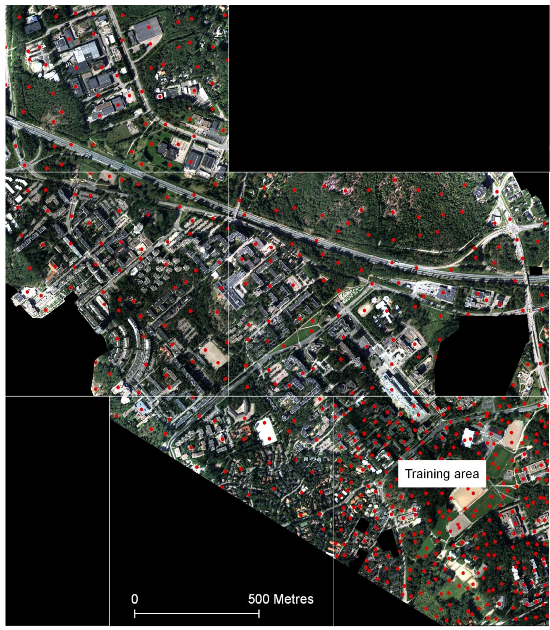
2.1. Study Area

The study area was located in Finland, in the suburban area of Espoonlahti, about 15 km from the centre of Helsinki. It was divided into five subareas including a training area of 0.7 km² and four validation areas covering 2.7 km² in total (see Figure 1). The training area was used for creating classification rules, and the separate validation areas were used for estimating the classification accuracy. Most of the study area is part of a high-rise residential area with some public and commercial buildings, but there is an industrial area in the north and a low-rise residential area in the southwest. In addition, there are smaller groups of low-rise buildings between the high-rise buildings. The area is partly covered by coniferous/mixed forest, and there are numerous trees all over the area. The main tree species are spruce, pine, and birch. The study area is part of a larger area that was used for building detection and change detection studies in [47].

The study area was delimited so that all of the datasets covered it and that no major changes in land cover occurred between the acquisition dates of the different datasets. Two subareas were excluded by using a manually defined mask because there were considerable changes in the land cover (the large black area and the small rectangular black area near the eastern border in Figure 1). In addition, three subareas were excluded from the training area by using a manually defined mask because there were gaps in the laser scanner data. These gaps were due to the low reflectance of the laser pulses from the roofs of some buildings. Smaller groups of empty pixels in the data derived from laser scanning were excluded automatically from all of the tests (these are also presented in black in Figure 1, but they are too small to be distinguished clearly). Depending on the dataset used, the processing of the area was carried out in one part (Tests 3 and 4, see Section 3.2) or five parts corresponding to the five subareas (Tests 1, 2, and 5).

2.2. Remotely Sensed Datasets

The datasets used in the present study included an aerial ortho image mosaic created from digital aerial images, digital surface models (DSMs) and associated data derived from laser scanning, a high-resolution optical QuickBird satellite image, and airborne E-SAR images. The characteristics of the E-SAR X-band images are similar to TerraSAR-X SpotLight satellite images. The fully polarimetric L-band data complement the X-band data and provide more information for classification. Unfortunately, very high resolution fully polarimetric L-band images are not available from the existing satellites. All of the datasets were processed for inclusion in the Finnish ETRS-TM35FIN coordinate system (ETRS is European Terrestrial Reference System, and TM is Transverse Mercator). The details of the datasets are presented in Table 3. The aerial image and laser scanner data were also used in [47] and the E-SAR data in [46,48]. In the prior studies, the E-SAR data were in an older coordinate system and for the present study they were transformed to the ETRS-TM35FIN coordinate system. The QuickBird image was rectified to this coordinate system by using a digital elevation model (DEM) produced by the National Land Survey of Finland.

Figure 1. Aerial ortho image mosaic of the study area and reference points (red dots). The training area was used for creating classification rules and the four validation areas (without labelling, separated by the white lines) were used for estimating the classification accuracy. The black areas were excluded.

Figure 1. Aerial ortho image mosaic of the study area and reference points (red dots). The training area was used for creating classification rules and the four validation areas (without labelling, separated by the white lines) were used for estimating the classification accuracy. The black areas were excluded.

Table 3. The datasets used in the classification tests.

Sensor	Acquisition date	Derived datasets in raster format	Pixel size	References
Intergraph DMC	1 September 2005	Aerial ortho image mosaic with red, green, blue, and near-infrared (NIR) channels (rectified by using a laser scanner derived DSM)	0.3 m × 0.3 m	[47]
Optech ALTM 3100 laser scanner	12 July 2005	Maximum DSM (maximum height for each pixel) Minimum DSM (minimum height) Maximum DSM – minimum DSM Morphologically filtered slope image calculated from the minimum DSM Height classification of laser points corresponding to the minimum DSM (ground, low, high (≥2.5 m from the ground), no laser points)	0.3 m × 0.3 m (original point density about 2–4 points/m2)	[49] (TerraScan software used to create the DSMs and point classification); [47] (general description of the data)
QuickBird	27 May 2003	Multispectral image with blue, green, red, and NIR channels (Off-nadir view angle of the sensor: 6.2°)	2 m × 2 m (resampled from the original 2.4 m)
E-SAR (DLR, German Aerospace Center)	2 May 2001	L-band (λ = 23 cm) image with four channels: LHH, LHV, LVV,( LVH*) X-band (λ = 3 cm) image with two channels XHH and XVV (Multilooked data: theoretical resolution about 2 m in range and about 3 m (L) or about 2 m (X) in azimuth direction) (Depression angle of the sensor: 40°)	1 m × 1 m (Test 4, see Section 3.2), resampled to 0.3 m (Test 5)	[48]

DMC = Digital Mapping Camera, ALTM = Airborne Laser Terrain Mapper, λ = wavelength; * The LVH channel was not used in tests because it is practically the same as LHV.

Table 3. The datasets used in the classification tests.

Sensor	Acquisition date	Derived datasets in raster format	Pixel size	References
Intergraph DMC	1 September 2005	Aerial ortho image mosaic with red, green, blue, and near-infrared (NIR) channels (rectified by using a laser scanner derived DSM)	0.3 m × 0.3 m	[47]
Optech ALTM 3100 laser scanner	12 July 2005	Maximum DSM (maximum height for each pixel) Minimum DSM (minimum height) Maximum DSM – minimum DSM Morphologically filtered slope image calculated from the minimum DSM Height classification of laser points corresponding to the minimum DSM (ground, low, high (≥2.5 m from the ground), no laser points)	0.3 m × 0.3 m (original point density about 2–4 points/m2)	[49] (TerraScan software used to create the DSMs and point classification); [47] (general description of the data)
QuickBird	27 May 2003	Multispectral image with blue, green, red, and NIR channels (Off-nadir view angle of the sensor: 6.2°)	2 m × 2 m (resampled from the original 2.4 m)
E-SAR (DLR, German Aerospace Center)	2 May 2001	L-band (λ = 23 cm) image with four channels: LHH, LHV, LVV,( LVH*) X-band (λ = 3 cm) image with two channels XHH and XVV (Multilooked data: theoretical resolution about 2 m in range and about 3 m (L) or about 2 m (X) in azimuth direction) (Depression angle of the sensor: 40°)	1 m × 1 m (Test 4, see Section 3.2), resampled to 0.3 m (Test 5)	[48]

DMC = Digital Mapping Camera, ALTM = Airborne Laser Terrain Mapper, λ = wavelength; * The LVH channel was not used in tests because it is practically the same as LHV.

2.3. Permanent Test Field Reference Points

In order to generate a permanent test field for land cover classification studies, reference points were collected over the Espoonlahti area by using a grid with 100 m × 100 m cells (see Figure 1). One point was set inside each grid cell so that it was located within a homogeneous region and the points were obtained from different classes. The points can be used as points, but they can also be converted into reference segments (especially training segments) after the segmentation of the image data. Segmentation defines the boundaries of the training segments, and it can be assumed that the entire segment belongs to the class defined by the point. This approach is flexible and allows the application of the same point set to define training segments for different types of image data. The characteristics of the training segments will vary depending on the data source, but the labelling is obtained from the single reference dataset.

The points were originally collected from an aerial colour ortho photo acquired in 2001, and they were used in [48]. Later on, the points were transformed to the ETRS-TM35FIN coordinate system and they were updated by using the ortho image mosaic and the laser scanner derived maximum DSM from 2005 (the same datasets that were used in the classification tests described here), a city base map from 2007, and a city plan from 2007. The positions of the points were improved so that they were better located within homogeneous areas, and changes in classification were made as needed. New points were collected in the training area by using a 50 m × 50 m grid to obtain enough training points.

Altogether 297 reference points from the training area were used for training and 269 points from the validation areas for estimating the accuracy of the classifications. The training points were further used to create training segments. The validation points were used as points. The reference points had object types (e.g., building, road, forest) and surface types (e.g., asphalt, gravel, tree canopy) as attributes (the surface types were not fully available). For the purpose of this classification study, the object types and surface types were generalised into four classes: building, tree, vegetated ground, and non-vegetated ground. The class ground also includes low vegetation such as grass or bushes and low objects such as cars visible in high-resolution datasets. Within forest there were some ground points that were located in small openings between trees (visible in the laser scanner DSM, but not clearly in the aerial ortho image). These points were considered as vegetated ground points when using laser scanner data and as tree points in other classification tests. The classes of the points correspond to the situation in 2005. The E-SAR data were acquired in 2001 and the QuickBird image in 2003, but the same classes were considered applicable because there were no major changes in land cover in the selected study area between 2001 and 2005. For a comparative study, we considered it best to use the same point set in each classification test.

3. Methods

3.1. Segmentation and Classification Methods

An object-based classification approach was used, which means that each dataset under analysis was segmented into homogeneous regions and various attributes for the segments were calculated. The multiresolution segmentation algorithm [50] of the eCognition software [51] was used. The segmentation results together with the segment attributes were exported from eCognition.

The classification of the segments was carried out by using the classification tree method [42] and the classification tree tools available in the Matlab Statistics Toolbox [52]. The reference points from the training area were used to define the training segments. If a reference point was inside a segment, the segment became a training segment of the corresponding class. A classification tree was then constructed automatically by using the classes and attributes of the training segments. Gini’s diversity index [42] was used as the splitting criterion to define the splits in the tree:

$$impurity(t)={\displaystyle \sum _{i\ne j}p(i}|t)p(j|t),$$

(1)

where t is a node in the tree, and p(i|t) is the proportion of cases x_n ℘ t belonging to class i (x is a vector of attributes for a training segment). When the tree is constructed, a search is made at each node of the tree for the split that reduces the node impurity the most. In our study, a node had to contain at least 10 training segments to be split (the default value). Pruning was used to avoid overfitting of training data. The best level of pruning was defined by computing the costs of the subtrees by using training data and 10-fold cross-validation. The costs were based on misclassifications produced by the trees. The best level suggested by the method was the level that produced the smallest tree within one standard error of the minimum-cost subtree. The suggested level may vary slightly between different cross-validation runs. Therefore, the computation was applied 10 times, and the level suggested in most of the runs was selected for classification. Further details of the classification tree construction and pruning can be found in [42,53].

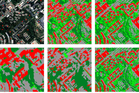
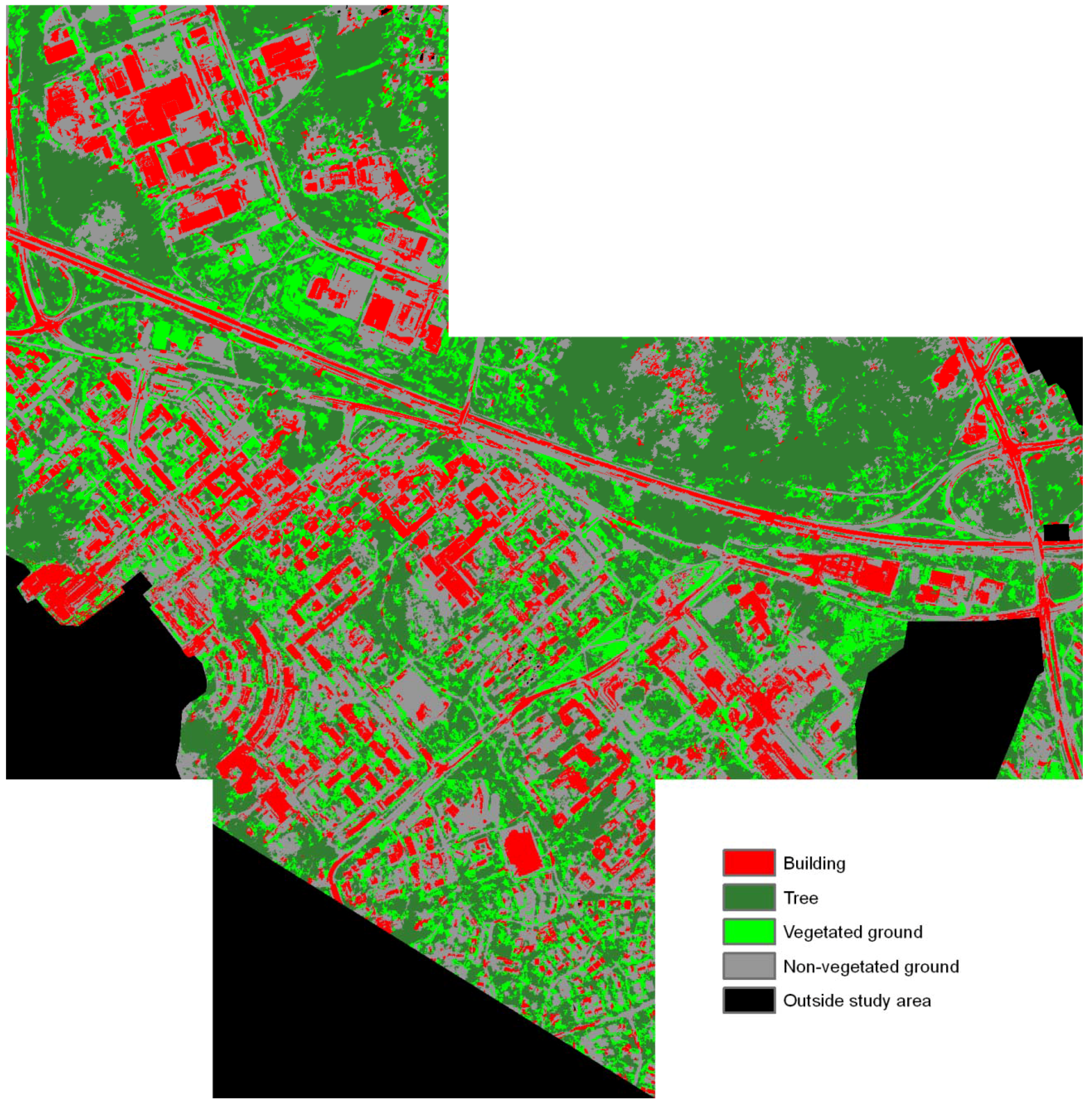
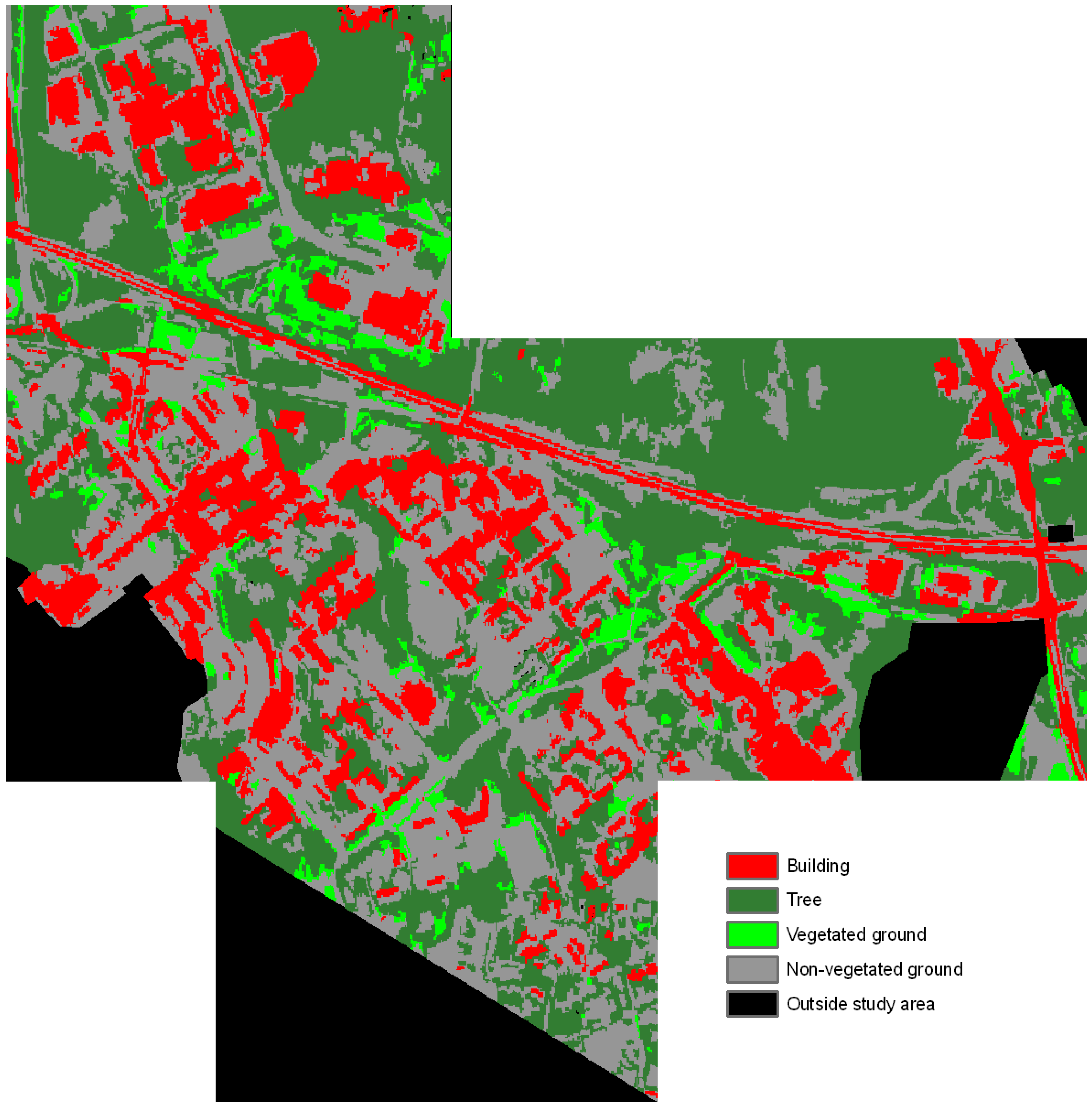
3.2. Classification Tests

Five classification tests were carried out by using the following datasets:

• Aerial ortho image mosaic
• Laser scanner derived datasets and aerial ortho image mosaic
• QuickBird image
• E-SAR image data
• Laser scanner derived datasets and E-SAR image data

The tested dataset combinations were selected on the basis of practical aspects. Laser scanner data were considered as optional additional data because they are not as commonly available and as frequently acquired as aerial or satellite imagery. If laser scanner data are available, they are typically combined with aerial imagery. This combination also represents the most optimal case considering the spatial resolution of the data. The combination of laser scanner data and SAR imagery is uncommon in practice, but it is interesting as a research topic because SAR data differ significantly from optical imagery.

Segmentation parameters were selected separately for each test on the basis of visual evaluation and previous experience, and they are presented in Table 4. In Classification Tests 2 and 5, two segmentation levels were produced: one based on the minimum DSM and the other based on the aerial image or E-SAR data. The second segmentation level was created below the first one, which meant that the DSM segments were further divided into smaller segments using the image data. The predefined height classification of the laser scanner data was used to divide the DSM segments into high objects and ground. If most of the laser points within a segment were high (≥2.5 m from ground level), the segment was classified as a high object, otherwise as ground. High objects and ground were then further classified in separate processes using the classification tree method: high objects into buildings and trees using the DSM segments and ground objects into vegetated and non-vegetated ground using the aerial image/E-SAR segments. The segment attributes calculated both from the image and laser scanner data were used in both steps. After classification of high objects, a postprocessing operation was also carried out to eliminate very small buildings (total area of the building < 20 m²). The classification of these objects was changed to tree, which is a more likely class for small, high objects.

Table 4. The segmentation parameters used in the different classification tests. For details of the parameters, see [54].

Classification test	Data used (weight)	Scale (determines segment size) *	Composition of homogeneity criterion
Test 1	Aerial ortho image mosaic: red (1), green (1), blue (1), NIR (1)	100	Colour 0.9, shape 0.1 (compactness 0.5, smoothness 0.5)
Test 2, high objects	Minimum DSM (1)	10	Colour 1, shape 0
Test 2, ground objects	Aerial ortho image mosaic: red (1), green (1), blue (1), NIR (1)	100	Colour 0.9, shape 0.1 (compactness 0.5, smoothness 0.5)
Test 3	QuickBird image: red (1), green (1), blue (1), NIR (1)	40	Colour 0.9, shape 0.1 (compactness 0.5, smoothness 0.5)
Test 4	E-SAR data: LHH (1), LHV (1), LVV (1), XHH (1), XVV (1)	80	Colour 0.5, shape 0.5 (compactness 0.5, smoothness 0.5)
Test 5, high objects	Minimum DSM (1)	10	Colour 1, shape 0
Test 5, ground objects	E-SAR data: LHH (1), LHV (1), LVV (1), XHH (1), XVV (1)	100	Colour 0.9, shape 0.1 (compactness 0.5, smoothness 0.5)

* An appropriate parameter value is dependent on the characteristics of each data source; e.g., on the numerical values in the data and pixel size. The parameters used in different tests are not directly comparable.

Table 4. The segmentation parameters used in the different classification tests. For details of the parameters, see [54].

Classification test	Data used (weight)	Scale (determines segment size) *	Composition of homogeneity criterion
Test 1	Aerial ortho image mosaic: red (1), green (1), blue (1), NIR (1)	100	Colour 0.9, shape 0.1 (compactness 0.5, smoothness 0.5)
Test 2, high objects	Minimum DSM (1)	10	Colour 1, shape 0
Test 2, ground objects	Aerial ortho image mosaic: red (1), green (1), blue (1), NIR (1)	100	Colour 0.9, shape 0.1 (compactness 0.5, smoothness 0.5)
Test 3	QuickBird image: red (1), green (1), blue (1), NIR (1)	40	Colour 0.9, shape 0.1 (compactness 0.5, smoothness 0.5)
Test 4	E-SAR data: LHH (1), LHV (1), LVV (1), XHH (1), XVV (1)	80	Colour 0.5, shape 0.5 (compactness 0.5, smoothness 0.5)
Test 5, high objects	Minimum DSM (1)	10	Colour 1, shape 0
Test 5, ground objects	E-SAR data: LHH (1), LHV (1), LVV (1), XHH (1), XVV (1)	100	Colour 0.9, shape 0.1 (compactness 0.5, smoothness 0.5)

* An appropriate parameter value is dependent on the characteristics of each data source; e.g., on the numerical values in the data and pixel size. The parameters used in different tests are not directly comparable.

3.3. Input Features for the Classification Tree Method

A large number of different segment attributes (features) were used as input data for the classification tree method in each classification test, and they are listed in Table 5 and Table 6. They included mean values, standard deviations, brightness, channel ratios, and texture attributes calculated from different image channels and DSM data. Geometric attributes describing the extent and shape of the segments were also used. The Normalized Difference Vegetation Index (NDVI) was calculated for the optical images and various channel ratios for the E-SAR data. The idea was to provide a wide selection of potentially useful features for the classification tree method, which selected automatically the most useful ones for the classification trees.

3.4. Accuracy Estimation

The classification accuracy for all of the classification results was calculated by using the reference points of the validation areas, i.e., excluding the training area. The accuracy estimates included completeness (corresponds to producer’s accuracy or interpretation accuracy), correctness (corresponds to user’s accuracy or object accuracy) and mean accuracy of individual classes, and the overall accuracy of the classification [55,56]. The mean accuracy for class i was calculated by using the equation presented by Helldén [56]:

$$Meanaccuracy(i)=\frac{2A}{B+C}100\%$$

(5)

where A is the number of correctly classified reference points for class i, B is the total number of reference points in class i in the reference data, and C is the total number of reference points classified into class i.

Table 5. The attributes given as the input data for the construction of the classification trees in the different classification tests (the list continues in Table 6). For details of the attributes, see [54].

Attributes for segments	Classification test
	1	2	3	4	5
Customized attributes
NDVI (calculated from mean values in the NIR and red channels)	×	×	×
LHH mean/LHV mean, LHH mean/LVV mean, LVV mean/LHV mean, XVV mean/LVV mean, XHH mean/LHH mean				×	×
Mean values
Red, green, blue, NIR	×	×	×
Maximum DSM, minimum DSM		×			×
Slope		×			×
LHH, LHV, LVV, XHH, XVV				×	×
Standard deviations
Red, green, blue, NIR	×	×	×
Maximum DSM, minimum DSM		×			×
Maximum DSM, minimum DSM		×			×
LHH, LHV, LVV, XHH, XVV				×	×
Brightness (Mean value of the mean values in the different channels)
Brightness based on red, green, blue, and NIR channels	×	×	×
Brightness based on LHH, LHV, and LVV channels				×	×
Ratios (Mean value in one channel divided by the sum of the mean values in all channels)
Red, green, blue, NIR	×	×	×

Table 5. The attributes given as the input data for the construction of the classification trees in the different classification tests (the list continues in Table 6). For details of the attributes, see [54].

Attributes for segments	Classification test
	1	2	3	4	5
Customized attributes
NDVI (calculated from mean values in the NIR and red channels)	×	×	×
LHH mean/LHV mean, LHH mean/LVV mean, LVV mean/LHV mean, XVV mean/LVV mean, XHH mean/LHH mean				×	×
Mean values
Red, green, blue, NIR	×	×	×
Maximum DSM, minimum DSM		×			×
Slope		×			×
LHH, LHV, LVV, XHH, XVV				×	×
Standard deviations
Red, green, blue, NIR	×	×	×
Maximum DSM, minimum DSM		×			×
Maximum DSM, minimum DSM		×			×
LHH, LHV, LVV, XHH, XVV				×	×
Brightness (Mean value of the mean values in the different channels)
Brightness based on red, green, blue, and NIR channels	×	×	×
Brightness based on LHH, LHV, and LVV channels				×	×
Ratios (Mean value in one channel divided by the sum of the mean values in all channels)
Red, green, blue, NIR	×	×	×

Table 6. The attributes given as the input data for the construction of the classification trees in the different classification tests (the list continues from Table 5). For details of the attributes, see [54].

Attributes for segments	Classification test
	1	2	3	4	5
Texture after Haralick: Grey Level Co-occurrence Matrix (GLCM) homogeneity, contrast, dissimilarity, entropy, angular 2nd moment, mean, standard deviation, and correlation; Grey Level Difference Vector (GLDV) angular 2nd moment and entropy
Red, green, blue, NIR	×	×	×
Maximum DSM, minimum DSM		×			×
LHH, LHV, LVV, XHH, XVV				×	×
Geometry, extent: area, border length, length, length/width, width	×	×	×	×	×
Geometry, shape: asymmetry, border index, compactness, density, elliptic fit, radius of largest enclosed ellipse, radius of smallest enclosing ellipse, rectangular fit, roundness, shape index	×	×	×	×	×
Geometry, shape based on polygons: Area (excluding inner polygons), area (including inner polygons), average length of edges, compactness, length of longest edge, number of edges, number of inner objects, perimeter, standard deviation of length of edges	×	×	×	×	×

Table 6. The attributes given as the input data for the construction of the classification trees in the different classification tests (the list continues from Table 5). For details of the attributes, see [54].

Attributes for segments	Classification test
	1	2	3	4	5
Texture after Haralick: Grey Level Co-occurrence Matrix (GLCM) homogeneity, contrast, dissimilarity, entropy, angular 2nd moment, mean, standard deviation, and correlation; Grey Level Difference Vector (GLDV) angular 2nd moment and entropy
Red, green, blue, NIR	×	×	×
Maximum DSM, minimum DSM		×			×
LHH, LHV, LVV, XHH, XVV				×	×
Geometry, extent: area, border length, length, length/width, width	×	×	×	×	×
Geometry, shape: asymmetry, border index, compactness, density, elliptic fit, radius of largest enclosed ellipse, radius of smallest enclosing ellipse, rectangular fit, roundness, shape index	×	×	×	×	×
Geometry, shape based on polygons: Area (excluding inner polygons), area (including inner polygons), average length of edges, compactness, length of longest edge, number of edges, number of inner objects, perimeter, standard deviation of length of edges	×	×	×	×	×

4. Results

The classification trees created automatically in the different tests are presented in Table 7 in the form of classification rules. It can be seen that the structure of the classification trees was simple and that the number of attributes used for classification was small compared to the total number of attributes available. In some cases, the trees were very simple with only one attribute tested. In Test 2, the classification of high objects into buildings and trees and the classification of ground objects into vegetated and non-vegetated ground were only based on NDVI thresholding. In Test 5, high objects were classified based only on DSM slope.

Table 7. The rules in the automatically created classification trees in the different classification tests.

Classification test	Rules in the classification tree
Test 1	IF Ratio NIR < 0.548739   IF Ratio NIR < 0.272026 → Building   ELSE     IF GLCM standard deviation blue < 40.6738       IF Density < 1.13185 → Non-vegetated ground       ELSE → Building     ELSE → Non-vegetated ground ELSE   IF GLCM standard deviation blue < 43.841     IF GLCM contrast green < 2386.87 → Vegetated ground     ELSE → Tree   ELSE → Tree
Test 2, high objects	IF NDVI < 0.441429 → Building ELSE → Tree
Test 2, ground objects	IF NDVI < 0.526306 → Non-vegetated ground ELSE → Vegetated ground
Test 3	IF NDVI < 0.358559   IF Ratio NIR < 0.256213 → Building   ELSE → Non-vegetated ground ELSE   IF Brightness < 263.028 → Tree   ELSE → Vegetated ground
Test 4	IF Mean LHH < 493.259   IF LVV mean/LHV mean < 2.37657 → Non-vegetated ground   ELSE → Vegetated ground ELSE   IF Standard deviation XHH < 227.942 → Tree   ELSE → Building
Test 5, high objects	IF Slope < 23.659 → Building ELSE → Tree
Test 5, ground objects	IF Mean XHH < 294.742 → Non-vegetated ground ELSE   IF Mean LHV < 131.277 → Vegetated ground   ELSE     IF GLCM Entropy min. DSM < 6.73737 → Non-vegetated ground     ELSE → Vegetated ground

Table 7. The rules in the automatically created classification trees in the different classification tests.

Classification test	Rules in the classification tree
Test 1	IF Ratio NIR < 0.548739   IF Ratio NIR < 0.272026 → Building   ELSE     IF GLCM standard deviation blue < 40.6738       IF Density < 1.13185 → Non-vegetated ground       ELSE → Building     ELSE → Non-vegetated ground ELSE   IF GLCM standard deviation blue < 43.841     IF GLCM contrast green < 2386.87 → Vegetated ground     ELSE → Tree   ELSE → Tree
Test 2, high objects	IF NDVI < 0.441429 → Building ELSE → Tree
Test 2, ground objects	IF NDVI < 0.526306 → Non-vegetated ground ELSE → Vegetated ground
Test 3	IF NDVI < 0.358559   IF Ratio NIR < 0.256213 → Building   ELSE → Non-vegetated ground ELSE   IF Brightness < 263.028 → Tree   ELSE → Vegetated ground
Test 4	IF Mean LHH < 493.259   IF LVV mean/LHV mean < 2.37657 → Non-vegetated ground   ELSE → Vegetated ground ELSE   IF Standard deviation XHH < 227.942 → Tree   ELSE → Building
Test 5, high objects	IF Slope < 23.659 → Building ELSE → Tree
Test 5, ground objects	IF Mean XHH < 294.742 → Non-vegetated ground ELSE   IF Mean LHV < 131.277 → Vegetated ground   ELSE     IF GLCM Entropy min. DSM < 6.73737 → Non-vegetated ground     ELSE → Vegetated ground

The classification results, confusion matrices, and accuracy estimates for each test are shown in Figure 2, Figure 3, Figure 4, Figure 5 and Figure 6 and Table 8, Table 9, Table 10, Table 11 and Table 12.

Figure 2. The results of Classification Test 1 (aerial ortho image data).

Figure 2. The results of Classification Test 1 (aerial ortho image data).

Table 8. The confusion matrix and accuracy estimates for Classification Test 1.

Classification	Reference (validation points)					Correctness
	Building	Tree	Vegetated ground	Non-vegetated ground	Sum
Building	44	0	0	38	82	53.7%
Tree	0	52	6	1	59	88.1%
Vegetated ground	2	3	20	1	26	76.9%
Non-vegetated ground	12	1	5	84	102	82.4%
Sum	58	56	31	124	269
Completeness	75.9%	92.9%	64.5%	67.7%
Mean accuracy	62.9%	90.4%	70.2%	74.3%
Overall accuracy	74.3%

Table 8. The confusion matrix and accuracy estimates for Classification Test 1.

Classification	Reference (validation points)					Correctness
	Building	Tree	Vegetated ground	Non-vegetated ground	Sum
Building	44	0	0	38	82	53.7%
Tree	0	52	6	1	59	88.1%
Vegetated ground	2	3	20	1	26	76.9%
Non-vegetated ground	12	1	5	84	102	82.4%
Sum	58	56	31	124	269
Completeness	75.9%	92.9%	64.5%	67.7%
Mean accuracy	62.9%	90.4%	70.2%	74.3%
Overall accuracy	74.3%

Figure 3. The results of Classification Test 2 (laser scanner and aerial ortho image data).

Figure 3. The results of Classification Test 2 (laser scanner and aerial ortho image data).

Table 9. The confusion matrix and accuracy estimates for Classification Test 2.

Classification	Reference (validation points)					Correctness
	Building	Tree	Vegetated ground	Non-vegetated ground	Sum
Building	54	0	0	0	54	100%
Tree	2	41	0	0	43	95.3%
Vegetated ground	0	2	42	1	45	93.3%
Non-vegetated ground	2	0	2	123	127	96.9%
Sum	58	43	44	124	269
Completeness	93.1%	95.3%	95.5%	99.2%
Mean accuracy	96.4%	95.3%	94.4%	98.0%
Overall accuracy	96.7%

Table 9. The confusion matrix and accuracy estimates for Classification Test 2.

Classification	Reference (validation points)					Correctness
	Building	Tree	Vegetated ground	Non-vegetated ground	Sum
Building	54	0	0	0	54	100%
Tree	2	41	0	0	43	95.3%
Vegetated ground	0	2	42	1	45	93.3%
Non-vegetated ground	2	0	2	123	127	96.9%
Sum	58	43	44	124	269
Completeness	93.1%	95.3%	95.5%	99.2%
Mean accuracy	96.4%	95.3%	94.4%	98.0%
Overall accuracy	96.7%

Figure 4. The results of Classification Test 3 (QuickBird image).

Figure 4. The results of Classification Test 3 (QuickBird image).

Table 10. The confusion matrix and accuracy estimates for Classification Test 3.

Classification	Reference (validation points)					Correctness
	Building	Tree	Vegetated ground	Non-vegetated ground	Sum
Building	41	0	0	44	85	48.2%
Tree	1	55	9	9	74	74.3%
Vegetated ground	0	0	16	2	18	88.9%
Non-vegetated ground	16	1	6	69	92	75.0%
Sum	58	56	31	124	269
Completeness	70.7%	98.2%	51.6%	55.6%
Mean accuracy	57.3%	84.6%	65.3%	63.9%
Overall accuracy	67.3%

Table 10. The confusion matrix and accuracy estimates for Classification Test 3.

Classification	Reference (validation points)					Correctness
	Building	Tree	Vegetated ground	Non-vegetated ground	Sum
Building	41	0	0	44	85	48.2%
Tree	1	55	9	9	74	74.3%
Vegetated ground	0	0	16	2	18	88.9%
Non-vegetated ground	16	1	6	69	92	75.0%
Sum	58	56	31	124	269
Completeness	70.7%	98.2%	51.6%	55.6%
Mean accuracy	57.3%	84.6%	65.3%	63.9%
Overall accuracy	67.3%

Figure 5. The results of Classification Test 4 (E-SAR data).

Figure 5. The results of Classification Test 4 (E-SAR data).

Table 11. The confusion matrix and accuracy estimates for Classification Test 4.

Classification	Reference (validation points)					Correctness
	Building	Tree	Vegetated ground	Non-vegetated ground	Sum
Building	24	1	0	5	30	80.0%
Tree	8	41	1	12	62	66.1%
Vegetated ground	2	0	22	10	34	64.7%
Non-vegetated ground	24	14	8	97	143	67.8%
Sum	58	56	31	124	269
Completeness	41.4%	73.2%	71.0%	78.2%
Mean accuracy	54.5%	69.5%	67.7%	72.7%
Overall accuracy	68.4%

Table 11. The confusion matrix and accuracy estimates for Classification Test 4.

Classification	Reference (validation points)					Correctness
	Building	Tree	Vegetated ground	Non-vegetated ground	Sum
Building	24	1	0	5	30	80.0%
Tree	8	41	1	12	62	66.1%
Vegetated ground	2	0	22	10	34	64.7%
Non-vegetated ground	24	14	8	97	143	67.8%
Sum	58	56	31	124	269
Completeness	41.4%	73.2%	71.0%	78.2%
Mean accuracy	54.5%	69.5%	67.7%	72.7%
Overall accuracy	68.4%

Figure 6. The results of Classification Test 5 (laser scanner and E-SAR data).

Figure 6. The results of Classification Test 5 (laser scanner and E-SAR data).

Table 12. The confusion matrix and accuracy estimates for Classification Test 5.

Classification	Reference (validation points)					Correctness
	Building	Tree	Vegetated ground	Non-vegetated ground	Sum
Building	54	0	0	0	54	100.0%
Tree	2	41	0	0	43	95.3%
Vegetated ground	1	0	34	32	67	50.7%
Non-vegetated ground	1	2	10	92	105	87.6%
Sum	58	43	44	124	269
Completeness	93.1%	95.3%	77.3%	74.2%
Mean accuracy	96.4%	95.3%	61.3%	80.3%
Overall accuracy	82.1%

Table 12. The confusion matrix and accuracy estimates for Classification Test 5.

Classification	Reference (validation points)					Correctness
	Building	Tree	Vegetated ground	Non-vegetated ground	Sum
Building	54	0	0	0	54	100.0%
Tree	2	41	0	0	43	95.3%
Vegetated ground	1	0	34	32	67	50.7%
Non-vegetated ground	1	2	10	92	105	87.6%
Sum	58	43	44	124	269
Completeness	93.1%	95.3%	77.3%	74.2%
Mean accuracy	96.4%	95.3%	61.3%	80.3%
Overall accuracy	82.1%

5. Discussion

5.1. Results of the Classification Tests

It is known from previous studies (e.g., [21,33]) that the quality of the classification results improves if height information from laser scanning is used in addition to aerial image data. This was also clearly evident in this study. The overall accuracies in Test 1 (aerial image data) and Test 2 (aerial image and laser scanner data) were 74% and 97%, respectively. These accuracy levels are comparable to those observed in other classification studies using aerial imagery and laser scanner data (Table 1 and Table 2), although it should be noted that direct comparisons of different studies are not possible because of different study areas, different reference datasets, and different class definitions.

In Test 1, the first rule in the classification tree separated non-vegetated and vegetated objects using the NIR channel (ratio to the sum of all channels). Non-vegetated segments were then classified into buildings and non-vegetated ground using the NIR ratio again, texture, and shape of the segments (attribute ‘density’, which is high for square objects). Trees and vegetated ground segments were classified by using texture attributes. There was some confusion between buildings and non-vegetated ground. This is not surprising when considering the relatively similar appearance of many building roofs and asphalt roads or gravel surfaces. In Test 1, there was also some confusion between trees and vegetated ground, but the mean accuracy of trees was as high as 90%. Some vegetated ground points were classified as non-vegetated. Most of these were located in areas with brownish vegetation in the ortho image. The aerial images used in this study were taken in the beginning of September. It should also be noted that there were some brightness variations in the ortho image mosaic because radiometric corrections were not applied in the preprocessing stage. Radiometric corrections could improve the classification results of the aerial image data.

When height information was used, confusion between buildings and non-vegetated ground could be effectively avoided. In Test 2, all of the accuracy estimates were clearly above 90% and very few errors occurred. Even vegetated and non-vegetated ground points were better distinguished from each other than in Test 1. Visually, some typical misclassifications could be found. For example, stretches of narrow roads have been misclassified as vegetated ground due to obscuring or shadowing trees. A few buildings with vegetation on their roofs were misclassified as trees. Overall, however, it seems that the simple NDVI rules worked well, once high and low objects had been separated by using the laser scanner data.

The overall accuracies in Test 3 (QuickBird image) and Test 4 (E-SAR data) were roughly the same, 67% and 68%. When compared, trees were classified better in Test 3 and ground was classified better in Test 4. It is difficult to say whether this was due to the different characteristics of the datasets or to the different acquisition times. In the present study, the lower resolution of the QuickBird and E-SAR data in comparison to the aerial image data is a probable cause for the classification accuracy being lower than in Test 1 and Test 2. For example, there is clearly more detail in the results of Test 1 (Figure 2) than in Test 3 (Figure 4). It should also be noted that the size of the segments was considerably larger in Test 3 and Test 4 when compared to Tests 1, 2, and 5; this was due to the coarser resolution of the input data. Furthermore, the amount of training segments was smaller in Test 3 (251) and Test 4 (260) because some segments contained several training points. Regarding the other tests, only a few such segments occurred (the number of training segments was 294 in Test 1, 296 in Test 2, and 295 in Test 5). The density of the training points was thus appropriate for the aerial image and laser scanner data, but rather high for the QuickBird and E-SAR data.

In Test 3, the classification tree first separated vegetated and non-vegetated segments based on NDVI. Buildings and non-vegetated ground were further classified based on the NIR ratio, and trees and vegetated ground based on brightness. The tree class had the highest accuracy and the building class the lowest accuracy, which was similar to the result in Test 1. As in Test 1, there was also confusion between buildings and non-vegetated ground; for example, the highway was classified as buildings. The QuickBird image was acquired in the end of May, and photographs acquired on site show that deciduous trees and bushes were not in full leaf then. On the other hand, the aerial image was acquired in September and undoubtedly shows more vegetation after the growing season and a higher contrast between vegetated and non-vegetated areas (e.g., NDVI and NIR ratio), although some of the vegetation was already brownish as discussed above. The QuickBird off-nadir view angle of 6.2° is not expected to affect the results, since the view angle is small, the QuickBird segments are large and the reference points were selected carefully in the middle of homogeneous areas.

In Test 4, the classification tree first distinguished the ground areas from buildings and trees, and this was different from the optical image classifications. This was carried out based on the LHH channel mean. Then ground areas were classified into vegetated and non-vegetated based on LVV/LHV. Trees and buildings were classified based on the XHH channel standard deviation. The class having the highest mean accuracy was non-vegetated ground, and the lowest mean accuracy was obtained for buildings. The reason for the low accuracy is that buildings in SAR images have special characteristics. The depression angle of the E-SAR sensor was 40°. Due to the side-looking image geometry, the vertical building walls cause geometric distortions (layover, foreshortening, shadow) in SAR images and strong double-bounce reflections on one side of the buildings [57]. In addition, the slope of the roof and the orientation of the building in relation to the imaging direction are significant. Therefore, buildings are visually detected in SAR images by bright (layover) areas and shadow areas next to the actual building. This is not always optimal for automated detection of buildings based on training points placed on roof tops. Shadows exist also in optical images, and as in SAR images, they can complicate the interpretation of areas next to buildings. Many buildings were classified as non-vegetated ground. This was probably caused by flat roofs that have similar SAR backscattering properties as flat non-vegetated ground areas. The test set also included small buildings, narrow roads, and other small non-vegetated areas, which could be covered by vegetation in the oblique SAR viewing direction. The E-SAR images were acquired in the beginning of May, and it is likely that there were no leaves on the trees and the vegetated ground had not yet begun to acquire vegetation. Therefore, the contrast between vegetated and non-vegetated ground was lower than later in the summer. Some trees could have been classified as ground as SAR occasionally images through the canopy, and the exact source of scattering depends on the radar wavelength and target properties. Trees and vegetated ground, however, were well separated from each other.

The accuracy of the E-SAR classification was lower than in [46], where the same image data were classified by using the classification tree method. This can be related to the reference points used for training and to the different classes of interest. In [46], the SAR imagery was used to define training points, which ensured that the points were correctly located (for example, a check was performed to ensure that the building points were located on buildings both in the SAR and in the aerial image data). The classes were water, forest, built-up, and open, which included both vegetated and non-vegetated areas. The results of other studies using optical satellite images and SAR images (Table 1) were also, to some extent, better than our test results. The main differences with respect to other studies on optical satellite data were that additional features (geometric activity and invariant moments) were used in other studies in classification and pan-sharpening was performed on the input images. RADARSAT-2 polarimetric data with resolution of 5–8 m and polarimetric target decomposition were used in the other SAR studies, and segmentation was performed on the Pauli image. Multitemporal SAR data and different viewing directions (ascending and descending) were used in [19]. However, it should also be noted that optimal classes can be selected in classification tests for a single data type. In addition, the reference samples are often selected from the data used and considering the characteristics of the data. With SAR images, problems involving buildings are often avoided by using the class built-up area instead of the class building.

The use of laser scanner data together with the SAR data clearly improved the results. In Test 5, high objects were classified based on the DSM slope only, and the accuracies of the classes building and tree were similar to the results obtained in Test 2. This also contributes to the overall accuracy of Test 5 (82%), which was significantly higher than in Test 4. The mean accuracy of vegetated ground decreased and the mean accuracy of non-vegetated ground increased. It should be noted that the E-SAR segments used in the classification of ground objects were relatively small, since they were segmented within small DSM segments. Considering the resolution of the E-SAR data, this was not optimal within the smallest segments.

The number of reference points in the different classes was not equal. Especially the number of non-vegetated ground points was large in the validation points, which emphasizes the effect of this class on overall accuracy. There were also differences in the number of training points. These effects, however, were basically similar in different tests.

5.2. Further Evaluation of the Results

In this study, accuracy estimation of the classification results was based on the 269 validation points located within homogeneous regions. For further evaluation of the results, more tests would be useful. For example, the use of map data would allow more extensive evaluation of classified objects.

To evaluate the adequacy of the validation points for the comparison purposes of this study, preliminary experiments with raster map data were carried out. Building vectors and road centre line vectors were used to create raster maps for one of the validation areas (left column, middle row in Figure 1). The percentage of building pixels classified as building and the percentage of road pixels classified as non-vegetated ground were calculated for each classification test. For buildings, the percentages were typically a few percentage units lower than completeness calculated from the validation points. The mutual order of the classification results, however, remained the same, i.e., the highest percentages were obtained in Tests 2 and 5, and the lowest in Test 4. In the case of roads, the percentages cannot be directly compared to the accuracy estimates calculated using the validation points (class non-vegetated ground also includes other objects than roads). However, the percentage in Test 2 was again the highest. The second best value was obtained in Test 5, followed by Test 1, Test 4, and Test 3. The results of these experiments were thus mainly in accordance with those obtained by using the validation points. The best classification results were clearly obtained in Tests 2 and 5. The exact numerical accuracy estimates, however, are likely to change if different reference data (e.g., map data) are used.

5.3. Feasibility of the Classification Tree Method and Permanent Test Field Points for a Comparative Study

The classification tree method and test field points provided a feasible means of comparing classification accuracy between different datasets. This method is highly automated and can easily provide a general idea on the relative quality and potential of different datasets. However, the accuracy level of the classifications was not very high, except in Tests 2 and 5 (buildings and trees). This is largely related to the input data and the available features, but other classification methods should also be tested in order to achieve optimal classification results. These could include further developments of the basic classification tree method, such as boosting or random forests (see [8,45,58,59]).

An important question associated with a permanent land cover classification test field is the applicability of the same reference points for different types of images. Basically, the same points can provide an objective basis for comparisons, but there are issues that can affect the analyses and should be considered in each study. The collection of reference points from specific data makes the point set optimal for that type of data (in this study aerial image and laser scanner data). Geometric differences between the datasets, such as the side-looking geometry of SAR sensors, complicate the problem. The spatial resolution of the datasets must also be taken into account. For example, individual buildings and narrow roads are not detectable at lower resolutions, and different class definitions would be needed. Another important question when using a permanent test field is the required updating frequency of the land cover information. It is dependent on the area and should be high enough to keep the data reliable. Ideally, to compare different datasets and their classification capabilities, the datasets should have the same resolution and be simultaneously acquired. However, simultaneous datasets are difficult to acquire since the sensors are not always available and clouds can prevent optical imaging.

We assume that in our study the above-mentioned issues were sufficiently under control to allow a comparison of the land cover classification capabilities of the datasets. All of the datasets had relatively high spatial resolution, and major changes in the land cover did not occur between the acquisitions dates of the data. The results for individual datasets, however, can be less optimal than in studies where training and validation data are specifically collected for each dataset (see the discussion related to SAR images in Section 5.1).

Another specific characteristic of the permanent test field approach is that shadows in SAR and optical images cannot be treated as a separate class, which is likely to cause some misclassifications. Permanent reference points for shadows cannot be collected because the locations of the shadows vary from one dataset to another. In practice, shadows in the datasets will overlap some of the reference points. This gives some information on the characteristics of the shadow areas in different land cover classes for the training of the classifier.

5.4. Practical Considerations

A high level of accuracy was achieved in Test 2 using laser scanner and aerial image data. It can be expected that this result could be a useful aid in practical map updating work. When compared visually with existing map data, it could yield information on the location of new and no longer existing buildings, forests, and roads. Roads were not separated from other non-vegetated ground objects in the classification, but they are easy to recognise visually from the results, except for the narrowest ones. In other tests, the accuracy and/or capability to detect small land cover features was lower than in Test 2. The E-SAR and QuickBird data would be better suited for coarser land cover monitoring applications.

Future research topics should include optimal combination of different optical and SAR datasets and more detailed classifications. Special attention should also be paid to optimal image acquisition times and features. For example, further research is needed on the effect of the season and spatial resolution on the classification results of aerial image and laser scanner data. The aerial images used in the present study were taken in September. Images used operationally for mapping in Finland are taken in the spring before there are leaves on deciduous trees. This time is the best for accurate mapping of objects such as buildings and roads, but it is not ideal for the classification of vegetated and non-vegetated objects. The spatial resolution of aerial ortho images produced operationally is typically about 0.5 m, which is slightly lower than the resolution in this study. Laser scanner data are also acquired in the spring and they have a lower point density than in this study (minimum point density 0.5 points/m²).

The NIR channel and NDVI were important features in the classification of optical images. In tests concerning SAR images, different image channels (polarization and wavelength) were also selected in the classification trees. The newer optical satellites have a very high resolution panchromatic channel (e.g., QuickBird data with 0.6 m resolution, GeoEye-1 and WorldView-2 data with 0.5 m resolution are commercially available) and lower resolution multispectral channels (e.g., QuickBird: 2.4 m, GeoEye-1 and WorldView-2: 2 m). Similarly, SAR satellites provide high-resolution single-polarization images, but multi-polarization images have lower resolution. Detailed classifications require very high resolution multichannel data, and these are not provided by satellites.

Height information clearly showed its potential for improving classifications. In addition to laser scanning, height information is available from aerial images by using photogrammetric techniques and SAR satellites by using SAR interferometry or radargrammetry. Height information from these datasets could also be used in land cover classifications. SAR image based height information is certainly less detailed than laser scanner data, but it is available globally and could be used for coarser land cover classifications. The TanDEM-X mission will provide a precise global DEM in a few years and more detailed elevation data can be extracted from individual images locally [60]. X-band SAR data can be used to produce DSMs. DSMs produced from aerial images could be used in detailed land cover classifications if up-to-date laser scanner data are not available.

In our study laser scanner data were used as additional data together with imagery. In previous studies, good land cover classification results have been obtained by using laser scanner data alone (e.g., [7,8]). Buildings, trees and ground (as one class) can even be classified by using information derived from height data alone (see, for example, [61], where the laser scanner dataset of the present study was used for building detection with and without aerial image data). In Test 5 of the present study, the classification of buildings, trees and ground was also based on height data (buildings and trees were separated by using DSM slope; see Table 7). For separating vegetated and non-vegetated ground, intensity information, which was not used in our study, would also be essential [7].

6. Conclusions

In order to better understand and exploit the rich information content of different remotely sensed datasets, there is a need for comparative land cover classification studies. In the present study, a fairly precise land cover map could be derived automatically by combining aerial image and laser scanner data (overall accuracy 97%). It is likely that this result could provide useful information for operational mapping applications. The lower resolution datasets (QuickBird and E-SAR) produced coarser classifications (67% and 68%). Very high resolution aerial images on their own were slightly better (74%). When laser scanning data were used to collaborate with SAR data, the results improved (82%).

The classification tree method and permanent test field points provided a feasible means of comparing the classification accuracy of different datasets. This method is highly automated and can easily provide a general idea on the relative quality and potential of different datasets. A general limitation of the approach is that the same reference points are not necessarily equally well suited for the analysis of different datasets with different spatial resolutions, geometric characteristics, and acquisition dates. Therefore, the results for individual datasets can be less optimal than in studies where training and validation data are specifically collected for each dataset.

In the present study, we concentrated on the comparison between different datasets and on a few basic land cover classes. Future research topics should include optimal combination of the different optical and SAR datasets, optimal input features, and more detailed classifications. Height information, which clearly showed its potential for improving classifications, can also be derived from aerial images and SAR satellite images. This would probably lead to better classifications of these datasets when additional laser scanner data are not available. To improve the accuracy of classifications, more advanced classification methods could also be tested.

References

1. Thomas, N.; Hendrix, C.; Congalton, R.G. A comparison of urban mapping methods using high-resolution digital imagery. Photogramm. Eng. Remote Sensing 2003, 69, 963–972. [Google Scholar]
2. Walter, V. Object-based classification of remote sensing data for change detection. ISPRS J. Photogramm. 2004, 58, 225–238. [Google Scholar] [CrossRef]
3. Kressler, F.P.; Franzen, M.; Steinnocher, K. Segmentation Based Classification of Aerial Images and Its Potential to Support the Update of Existing Land Use Data Bases. In Proceedings of the ISPRS Hannover Workshop 2005: High-Resolution Earth Imaging for Geospatial Information, Hannover, Germany, 17–20 May 2005; Available online: http://www.isprs.org/publications/related/hannover05/paper/papers.htm (accessed on 11 May 2011).
4. Sanchez Hernandez, C.; Gladstone, C.; Holland, D. Classification of Urban Features from Intergraph’s Z/I Imaging DMC High Resolution Images for Integration into a Change Detection Flowline within Ordnance Survey. In Proceedings of the 2007 IEEE Urban Remote Sensing Joint Event, URBAN 2007-URS 2007, Paris, France, 11–13 April 2007.
5. Xu, S.; Fang, T.; Li, D.; Wang, S. Object classification of aerial images with bag-of-visual words. IEEE Geosci. Remote Sens. Lett. 2010, 7, 366–370. [Google Scholar]
6. Brennan, R.; Webster, T.L. Object-oriented land cover classification of lidar-derived surfaces. Can. J. Remote Sens. 2006, 32, 162–172. [Google Scholar] [CrossRef]
7. Im, J.; Jensen, J.R.; Hodgson, M.E. Object-based land cover classification using high-posting-density LiDAR data. GISci. Remote Sens. 2008, 45, 209–228. [Google Scholar] [CrossRef]
8. Chehata, N.; Guo, L.; Mallet, C. Airborne Lidar Feature Selection for Urban Classification Using Random Forests. In Proceedings of the ISPRS Workshop: Laserscanning’09, Paris, France, 1–2 September 2009; In International Archives of Photogrammetry, Remote Sensing and Spatial Information Sciences. Volume XXXVIII, Part 3/W8, pp. 207–212.
9. Garcia-Gutierrez, J.; Gonçalves-Seco, L.; Riquelme-Santos, J.C. Decision Trees on Lidar to Classify Land Uses and Covers. In Proceedings of the ISPRS Workshop: Laserscanning’09, Paris, France, 1–2 September 2009; In International Archives of Photogrammetry, Remote Sensing and Spatial Information Sciences. Volume XXXVIII, Part 3/W8, pp. 323–328.
10. Zhang, Q.; Wang, J. A rule-based urban land use inferring method for fine-resolution multispectral imagery. Can. J. Remote Sens. 2003, 29, 1–13. [Google Scholar] [CrossRef]
11. Kux, H.J.H.; Araújo, E.H.G. Object-based image analysis using QuickBird satellite images and GIS data, case study Belo Horizonte (Brazil). In Object-Based Image Analysis: Spatial Concepts for Knowledge-Driven Remote Sensing Applications; Blaschke, T., Lang, S., Hay, G.J., Eds.; Springer: Berlin, Germany, 2008; pp. 571–588. [Google Scholar]
12. Lackner, M.; Conway, T.M. Determining land-use information from land cover through an object-oriented classification of IKONOS imagery. Can. J. Remote Sens. 2008, 34, 77–92. [Google Scholar] [CrossRef]
13. Chan, J.C.-W.; Bellens, R.; Canters, F.; Gautama, S. An assessment of geometric activity features for per-pixel classification of urban man-made objects using very high resolution satellite imagery. Photogramm. Eng. Remote Sensing 2009, 75, 397–411. [Google Scholar] [CrossRef]
14. Bouziani, M.; Goita, K.; He, D.-C. Rule-based classification of a very high resolution image in an urban environment using multispectral segmentation guided by cartographic data. IEEE Trans. Geosci. Remote Sens. 2010, 48, 3198–3211. [Google Scholar] [CrossRef]
15. Xu, H.; Li, P. Urban land cover classification from very high resolution imagery using spectral and invariant moment shape information. Can. J. Remote Sens. 2010, 36, 248–260. [Google Scholar] [CrossRef]
16. Corr, D.G.; Walker, A.; Benz, U.; Lingenfelder, I.; Rodrigues, A. Classification of Urban SAR Imagery Using Object Oriented Techniques. In Proceedings of IGARSS ’03, Toulouse, France, 21–25 July 2003; Volume 1, pp. 188–190.
17. Chaabouni-Chouayakh, H.; Datcu, M. Coarse-to-fine approach for urban area interpretation using TerraSAR-X data. IEEE Geosci. Remote Sens. Lett. 2010, 7, 78–82. [Google Scholar] [CrossRef]
18. Li, X.; Pottier, E.; Guo, H.; Ferro-Famil, L. Urban land cover classification with high-resolution polarimetric SAR interferometric data. Can. J. Remote Sens. 2010, 36, 236–247. [Google Scholar] [CrossRef]
19. Niu, X.; Ban, Y. Multitemporal RADARSAT-2 Polarimetric SAR Data for Urban Land-Cover Mapping. In Proceedings of the ISPRS Technical Commission VII Symposium: 100 Years ISPRS Advancing Remote Sensing Science, Vienna, Austria, 5–7 July 2010; In International Archives of Photogrammetry, Remote Sensing and Spatial Information Sciences. Volume XXXVIII, Part 7A, pp. 175–180.
20. Qi, Z.; Yeh, A.G.; Li, X.; Lin, Z. Land Use and Land Cover Classification Using RADARSAT-2 Polarimetric SAR Image. In Proceedings of the ISPRS Technical Commission VII Symposium: 100 Years ISPRS Advancing Remote Sensing Science, Vienna, Austria, 5–7 July 2010; In International Archives of Photogrammetry, Remote Sensing and Spatial Information Sciences. Volume XXXVIII, Part 7A, pp. 198–203.
21. Gamba, P.; Houshmand, B. Joint analysis of SAR, LIDAR and aerial imagery for simultaneous extraction of land cover, DTM and 3D shape of buildings. Int. J. Remote Sens. 2002, 23, 4439–4450. [Google Scholar] [CrossRef]
22. Huang, M.-J.; Shyue, S.-W.; Lee, L.-H.; Kao, C.-C. A knowledge-based approach to urban feature classification using aerial imagery with lidar data. Photogramm. Eng. Remote Sensing 2008, 74, 1473–1485. [Google Scholar] [CrossRef]
23. Chen, Y.; Su, W.; Li, J.; Sun, Z. Hierarchical object oriented classification using very high resolution imagery and LIDAR data over urban areas. Adv. Space Res. 2009, 43, 1101–1110. [Google Scholar] [CrossRef]
24. Ban, Y.; Hu, H.; Rangel, I.M. Fusion of Quickbird MS and RADARSAT SAR data for urban land-cover mapping: Object-based and knowledge-based approach. Int. J. Remote Sens. 2010, 31, 1391–1410. [Google Scholar] [CrossRef]
25. Bellmann, A.; Hellwich, O. Sensor and data fusion contest: Information for mapping from airborne SAR and optical imagery (Phase I). In EuroSDR Official Publication No 50; EuroSDR: Frankfurt, Germany, 2006; pp. 183–215. [Google Scholar]
26. Schistad Solberg, A.H.; Jain, A.K.; Taxt, T. Multisource classification of remotely sensed data: Fusion of Landsat TM and SAR images. IEEE Trans. Geosci. Remote Sens. 1994, 32, 768–778. [Google Scholar] [CrossRef]
27. Kuplich, T.M.; Freitas, C.C.; Soares, J.V. The study of ERS-1 SAR and Landsat TM synergism for land use classification. Int. J. Remote Sens. 2000, 21, 2101–2111. [Google Scholar] [CrossRef]
28. Amarsaikhan, D.; Ganzorig, M.; Ache, P.; Blotevogel, H. The integrated use of optical and InSAR data for urban land-cover mapping. Int. J. Remote Sens. 2007, 28, 1161–1171. [Google Scholar] [CrossRef]
29. Pacifici, F.; Del Frate, F.; Emery, W.J.; Gamba, P.; Chanussot, J. Urban mapping using coarse SAR and optical data: Outcome of the 2007 GRSS data fusion contest. IEEE Geosci. Remote Sens. Lett. 2008, 5, 331–335. [Google Scholar] [CrossRef]
30. Riedel, T.; Thiel, C.; Schmullius, C. Fusion of multispectral optical and SAR images towards operational land cover mapping in Central Europe. In Object-Based Image Analysis: Spatial Concepts for Knowledge-Driven Remote Sensing Applications; Blaschke, T., Lang, S., Hay, G.J., Eds.; Springer: Berlin, Germany, 2008; pp. 493–511. [Google Scholar]
31. Hellwich, O.; Günzl, M.; Wiedemann, C. Fusion of SAR/INSAR data and optical imagery for landuse classification. Frequenz 2001, 55, 129–136. [Google Scholar] [CrossRef]
32. Amarsaikhan, D.; Blotevogel, H.H.; van Genderen, J.L.; Ganzorig, M.; Gantuya, R.; Nergui, B. Fusing high-resolution SAR and optical imagery for improved urban land cover study and classification. Int. J. Image Data Fusion 2010, 1, 83–97. [Google Scholar] [CrossRef]
33. Haala, N.; Brenner, C. Extraction of buildings and trees in urban environments. ISPRS J. Photogramm. 1999, 54, 130–137. [Google Scholar] [CrossRef]
34. Hodgson, M.E.; Jensen, J.R.; Tullis, J.A.; Riordan, K.D.; Archer, C.M. Synergistic use of lidar and color aerial photography for mapping urban parcel imperviousness. Photogramm. Eng. Remote Sensing 2003, 69, 973–980. [Google Scholar] [CrossRef]
35. Rottensteiner, F.; Trinder, J.; Clode, S.; Kubik, K. Using the Dempster-Shafer method for the fusion of LIDAR data and multi-spectral images for building detection. Inf. Fusion 2005, 6, 283–300. [Google Scholar] [CrossRef]
36. Zhou, W.; Troy, A. An object-oriented approach for analysing and characterizing urban landscape at the parcel level. Int. J. Remote Sens. 2008, 29, 3119–3135. [Google Scholar] [CrossRef]
37. Hofmann, P. Detecting buildings and roads from IKONOS data using additional elevation information. GeoBITGIS 2001, 6, 28–33. [Google Scholar]
38. Kettig, R.L.; Landgrebe, D.A. Classification of multispectral image data by extraction and classification of homogeneous objects. IEEE Trans. Geosci. Electron. 1976, GE-14, 19–26. [Google Scholar] [CrossRef]
39. Blaschke, T.; Lang, S.; Hay, G.J. Object-Based Image Analysis: Spatial Concepts for Knowledge-Driven Remote Sensing Applications; Springer: Berlin, Germany, 2008. [Google Scholar]
40. Blaschke, T. Object based image analysis for remote sensing. ISPRS J. Photogramm. 2010, 65, 2–16. [Google Scholar] [CrossRef]
41. Addink, E.A.; Van Coillie, F.M.B. Geographic Object-Based Image Analysis. In Proceedings of GEOBIA 2010, Ghent, Belgium, 29 June–2 July 2010; Available online: http://geobia.ugent.be/proceedings/ (accessed on 11 May 2011).
42. Breiman, L.; Friedman, J.H.; Olshen, R.A.; Stone, C.J. Classification and Regression Trees; Wadsworth, Inc.: Belmont, CA, USA, 1984. [Google Scholar]
43. Friedl, M.A.; Brodley, C.E. Decision tree classification of land cover from remotely sensed data. Remote Sens. Environ. 1997, 61, 399–409. [Google Scholar] [CrossRef]
44. Lawrence, R.L.; Wright, A. Rule-based classification systems using classification and regression tree (CART) analysis. Photogramm. Eng. Remote Sensing 2001, 67, 1137–1142. [Google Scholar]
45. Mancini, A.; Frontoni, E.; Zingaretti, P. Automatic Extraction of Urban Objects from Multi-Source Aerial Data. In Proceedings of CMRT09: Object Extraction for 3D City Models, Road Databases and Traffic Monitoring—Concepts, Algorithms and Evaluation, Paris, France, 3–4 September 2009; In International Archives of Photogrammetry, Remote Sensing and Spatial Information Sciences. Volume XXXVIII, Part 3/W4, pp. 13–18.
46. Matikainen, L. Improving automation in rule-based interpretation of remotely sensed data by using classification trees. Photogramm. J. Fin. 2006, 20, 5–20. [Google Scholar]
47. Matikainen, L.; Hyyppä, J.; Ahokas, E.; Markelin, L.; Kaartinen, H. Automatic detection of buildings and changes in buildings for updating of maps. Remote Sens. 2010, 2, 1217–1248. [Google Scholar] [CrossRef]
48. Matikainen, L.; Karjalainen, M.; Kaartinen, H.; Hyyppä, J. Rule-based interpretation of high-resolution SAR images for map updating. Photogramm. J. Fin. 2004, 19, 47–62. [Google Scholar]
49. Terrasolid. Homepage; Terrasolid Ltd.: Helsinki, Finland. Available online: http://www.terrasolid.fi/ (accessed on 11 May 2011).
50. Baatz, M.; Schäpe, A. Multiresolution segmentation—An optimization approach for high quality multi-scale image segmentation. In Angewandte Geographische Informationsverarbeitung XII: Beiträge zum AGIT-Symposium Salzburg 2000; Strobl, J., Blaschke, T., Griesebner, G., Eds.; Wichmann: Heidelberg, Germany, 2000; pp. 12–23. [Google Scholar]
51. Trimble GeoSpatial. Homepage; Trimble GeoSpatial: Munich, Germany. Available online: http://www.ecognition.com/ (accessed on 11 May 2011).
52. The MathWorks. Homepage; The MathWorks, Inc.: Natick, MA, USA. Available online: http://www.mathworks.com/ (accessed on 11 May 2011).
53. The MathWorks. Online Documentation for Statistics Toolbox; Version 6.1; The MathWorks, Inc.: Natick, MA, USA, 2007. [Google Scholar]
54. Definiens. Definiens eCognition 8.0.1 Reference Book; Definiens AG: München, Germany, 2010. [Google Scholar]
55. Congalton, R.G.; Green, K. Assessing the Accuracy of Remotely Sensed Data: Principles and Practices; Lewis Publishers: Boca Raton, FL, USA, 1999. [Google Scholar]
56. Helldén, U. A Test of Landsat-2 Imagery and Digital Data for Thematic Mapping, Illustrated by an Environmental Study in Northern Kenya; Rapporter och Notiser 47; University of Lund: Lund, Sweden, 1980. [Google Scholar]
57. Schreier, G. Geometrical properties of SAR images. In SAR Geocoding: Data and Systems; Schreier, G., Ed.; Wichmann: Karlsruhe, Germany, 1993; pp. 103–134. [Google Scholar]
58. Breiman, L. Random forests. Mach. Learn. 2001, 45, 5–32. [Google Scholar] [CrossRef]
59. Lawrence, R.; Bunn, A.; Powell, S.; Zambon, M. Classification of remotely sensed imagery using stochastic gradient boosting as a refinement of classification tree analysis. Remote Sens. Environ. 2004, 90, 331–336. [Google Scholar] [CrossRef]
60. Krieger, G.; Moreira, A.; Fiedler, H.; Hajnsek, I.; Werner, M.; Younis, M.; Zink, M. TanDEM-X: A satellite formation for high-resolution SAR interferometry. IEEE Trans. Geosci. Remote Sens. 2007, 45, 3317–3341. [Google Scholar] [CrossRef]
61. Matikainen, L.; Hyyppä, J.; Ahokas, E.; Markelin, L.; Kaartinen, H. An Improved Approach for Automatic Detection of Changes in Buildings. In Proceedings of the ISPRS Workshop: Laserscanning’09, Paris, France, 1–2 September 2009; In International Archives of Photogrammetry, Remote Sensing and Spatial Information Sciences. Volume XXXVIII, Part 3/W8, pp. 61–67.