1. Introduction
Airborne laser scanning (ALS) has become one of the most popular methods for collecting three-dimensional (3D) data to construct digital terrain models (DTM), digital surface models (DSM) and other end-products derived from these two main products. 3D coordinates of ALS point clouds can be directly georeferenced through a vector summation process, presuming that these vectors have already been rotated with regard to the relative orientations between target and inertial measurement unit (IMU) coordinates, laser and IMU units and the direction of the laser beam in relation to the laser unit [
1]. External orientation between the platform and target coordinate system,
i.e., direct georeferencing of the system, is solved using both GPS and inertial measurements. Because ALS systems include many components, accurate system calibration is necessary. System calibration determines the relative orientations between all of the sensors [
2] and compensates for other errors that are typical of ALS components [
3].
In practice, laser scanning strips of a larger scanning campaign require post-processing to ensure that data quality is adequate. Typically, ALS data is corrected using a strip adjustment procedure [
4,
5,
6] that requires overlapping adjacent and across-track strips and/or ground truth information. However, ground truth information is needed for an absolute verification of ALS data accuracy [
7]. One approach for improving accuracy involves direct correction of the physical calibration parameters of the laser scanning system; however, this approach requires knowledge of existing trajectory data information. An alternative solution involves estimation of a strip-wise correction of ALS data using ground control features; in this case, the corrections are added directly to the 3D ALS point clouds [
8]. For example, the process of exploiting ground truth information can involve comparison to different reference surfaces [
9,
10,
11] as well as to ALS-specific ground control targets that are validated in engineering scale mapping applications [
12]. Additionally, the utility of tacheometer and real-time kinematic (RTK) point measurements and pavement markings as ground truth information for ALS systems have been investigated [
13,
14,
15].
Currently, GPS can be accessed in real time using carrier-wave interferometry (RTK measurements) to obtain centimeter-precision positions. Easy visibility to most of the sky is required such that at least five satellites are almost continuously in view. Therefore, urban canyons or forests may be obstacles to collecting accurate GPS measurements. Despite occasional blockages, existing software is able to provide positions using reference objects in the landscape. The RTK technique presupposes the use of a base station in a known location, thereby allowing the roving GPS receiver to be corrected in real time. Alternatively, one can subscribe to a virtual reference station (VRS) service that conceptually provides the same information for a computationally constructed base station, which is based on a network of stations in known locations that are close to the roving user. The advantage of the VRS service is that base stations are not needed, and thus ground control points are not needed near measurement areas. The quality of GPS measurements is affected by errors in estimating the satellite clocks, ionospheric and tropospheric refraction errors, ephemeris errors, and multi-path reflections, providing a position accuracy of several centimeters.
The objective of this paper is to assess the feasibility of using vehicle-borne GPS measurements to evaluate the correctness of ALS point cloud heights. Both mobile RTK and VRS GPS methods were utilized; consequently, our practical examples highlight differences and similarities between RTK and VRS GPS measuring methods. Roads were selected as tie features because good coverage can be obtained, the surfaces are approximately level and data acquisition is rapid using mobile GPS systems.
2. Materials
The test area was located in Klaukkala (24°23′50″, 60°23′50″) 30 km north of Helsinki. ALS data were acquired in 2008 by the National Land Survey (NLS) of Finland with a minimum point density of 0.5 points per m
2. Currently, a nation-wide digital terrain model (DTM) that has an accuracy requirement of 30 cm is the primary product obtained from ALS data. The specified nominal vertical accuracy of the point data is 15 cm. The laser scan data were transformed into the EUREF-FIN/TM35FIN coordinate system [
16] and the N2000 vertical datum using the FIN2005 geoid model [
17]. The FIN2005 model is based on the Nordic NKG2004 geoid model. Post-processing was performed by the National Land Survey of Finland [
18] using strip adjustment and georeferencing.
Dual frequency Topcon HiPer Pro GPS+ receivers were used with a Topcon FC100 field computer and TopSurv software version 6.11.02. According to the manufacturer, the horizontal accuracy of this device is 1 cm plus 1 part per million (ppm) times the baseline distance, and the vertical accuracy is 1.5 cm plus 0.5 ppm times the baseline distance. The GPS receiver was mounted on top of a vehicle.
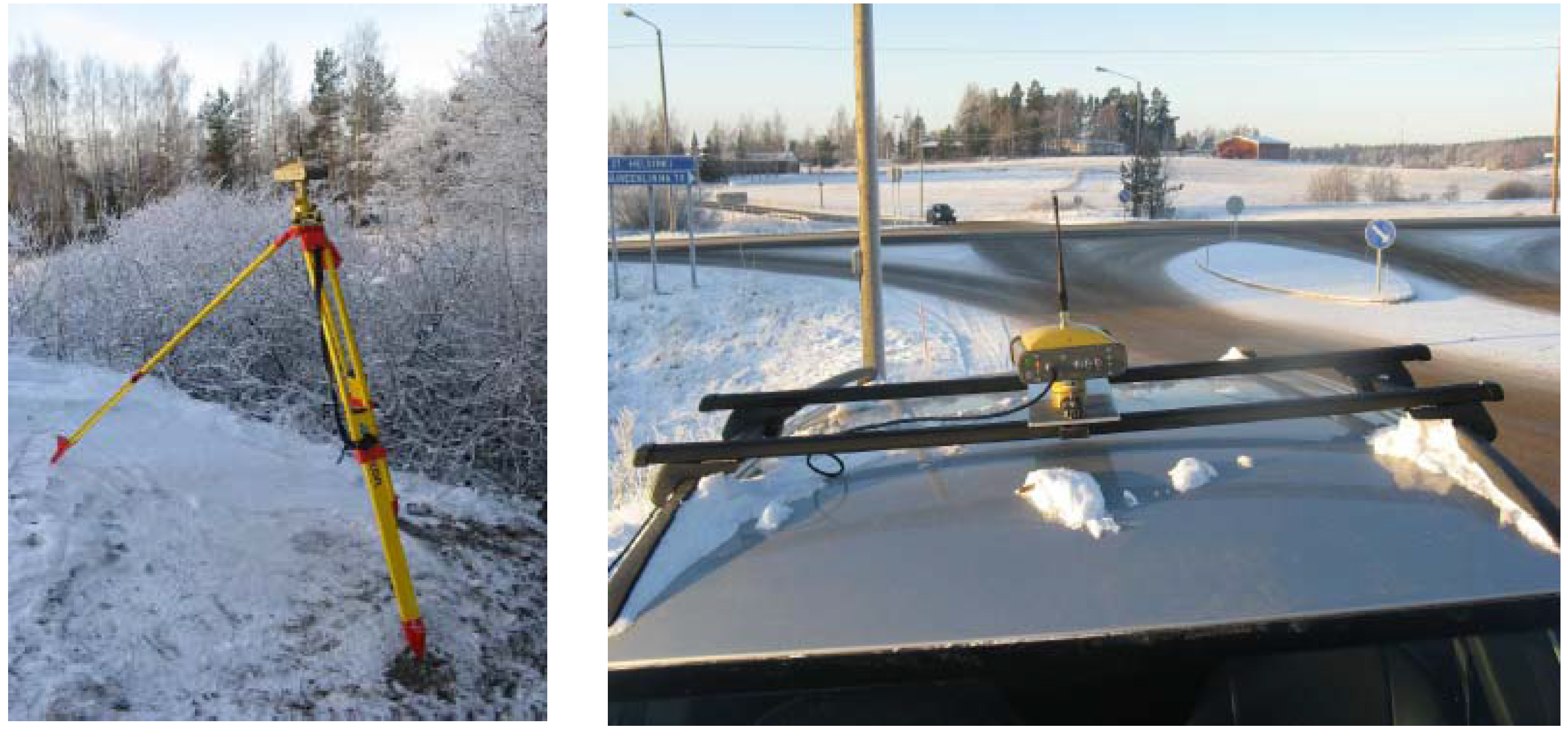
Figure 1 illustrates the measurement collection set-up. The 20-channel receivers tracked both GPS and GLONASS satellites. For RTK measurements, the same base station served the entire test area. For VRS GPS measurements, the GNSSnet.fi service was used.
Figure 1.
A Topcon HiPer Pro GPS+ receiver is shown on the reference point (left) and mounted on the top of the vehicle (right). (Photo: Panu Salo).
Figure 1.
A Topcon HiPer Pro GPS+ receiver is shown on the reference point (left) and mounted on the top of the vehicle (right). (Photo: Panu Salo).
3. Methods
3.1. GPS Vehicle Installation
The GPS antenna was attached to the roof rack of a vehicle as illustrated in
Figure 1. The height of the antenna from the road surface was measured, accounting for the effect of the weights of the driver and passengers. The antenna height above the road surface was accounted for during GPS processing; therefore, the output referred directly to the road surface, and comparison with ALS point data can be performed directly.
To find the distance between the GPS receiver and the road surface, the GPS receiver was mounted temporarily at the top of the measuring rod. The measuring rod with the attached GPS was moved close to each vehicle tire and leveled for each measurement. GPS measurements were thus obtained from different sides of the vehicle; the length of the measuring rod was subsequently subtracted from the GPS height values, and the average height was calculated to determine the height of the road surface. This method assumed that the road is close to a plane. In the next step, the GPS receiver was mounted on the roof rack of the vehicle. The receiver was centered relative to the four tires, and the distance between the road surface and GPS antenna was determined by subtracting the previously measured height of the road surface from the GPS observation reported for the position on the roof rack. Later, this distance was utilized when all of the observed, moving GPS measurements were referenced to the road surface. The method used to measure the distance between the road surface and the antenna is illustrated in
Figure 2.
Figure 2.
Determination of the distance between the road surface and the GPS antenna. The height level of the road was measured close to each tire. These four measurements were averaged to obtain an estimate for the general level of the ground surface. Next, this height value was subtracted from the observed height value of the GPS receiver mounted on the top of the vehicle.
If the vehicle is not level during data acquisition, a small error is generated, due to the drop in the GPS observation directly downwards relative to the GPS height calibration. In these cases, the angle of the vehicle should be taken into account when determining the corrected heights. However, the road slopes in our test area were not steep enough to require this kind of correction.
3.2. GPS System Measurements
GPS measurements were collected as the vehicle was driven along the test roads. The distribution of the roads used for measurement collection is illustrated in
Figure 3 and
Figure 4. The weather during measurement collection was clear. Testing occurred during the winter season, and the temperature was −20 °C; however, the majority of the road surfaces had negligible or no snow cover.
Figure 3.
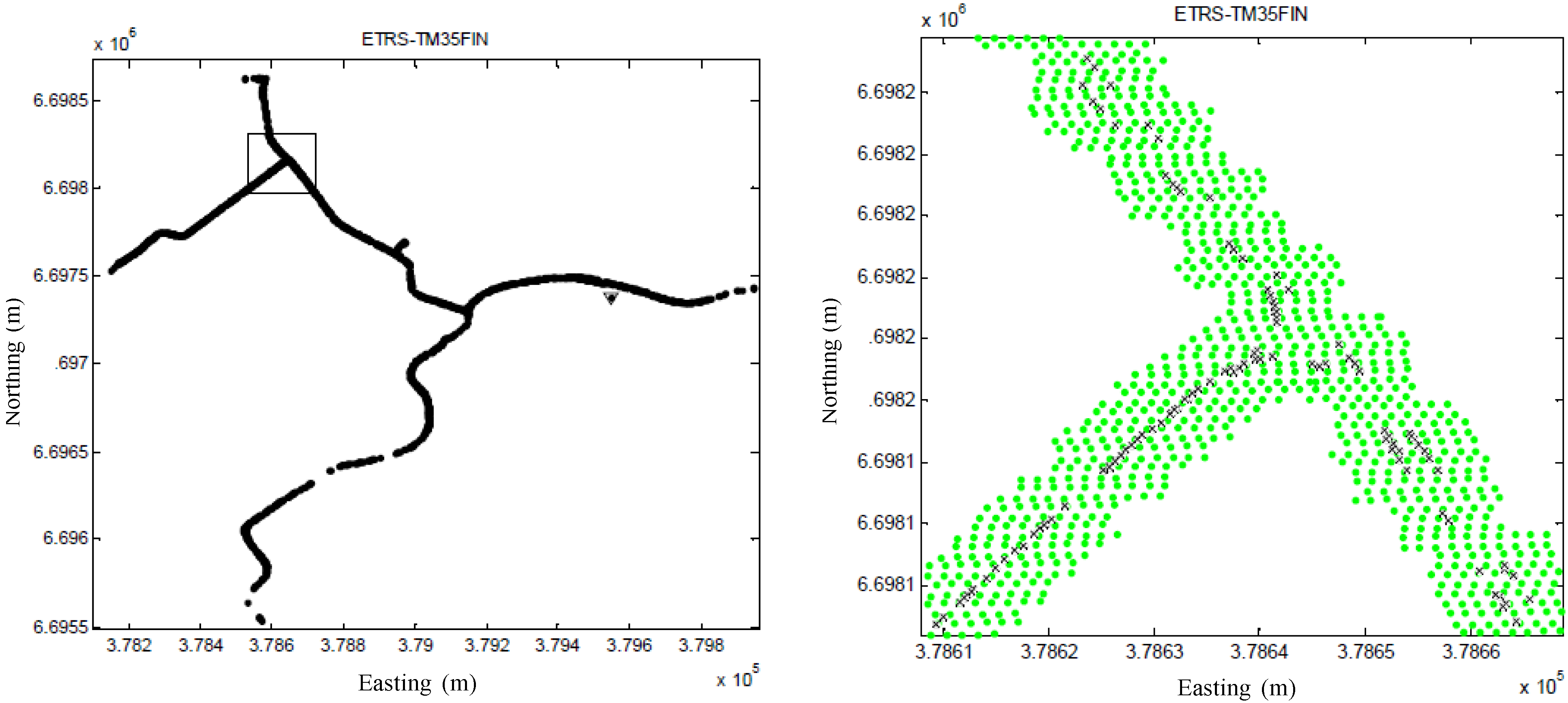
Virtual reference station (VRS) GPS observations along the test area roads. Left: The complete test area. The VRS virtual reference station was provided by Geotrim Oy (GNSSNet.fi). Right: A detailed view from the test area (the area marked with a square in the left image). GPS observations are illustrated with black crosses, and airborne laser scanning (ALS) points near GPS observations are represented by green dots.
Figure 3.
Virtual reference station (VRS) GPS observations along the test area roads. Left: The complete test area. The VRS virtual reference station was provided by Geotrim Oy (GNSSNet.fi). Right: A detailed view from the test area (the area marked with a square in the left image). GPS observations are illustrated with black crosses, and airborne laser scanning (ALS) points near GPS observations are represented by green dots.
Figure 4.
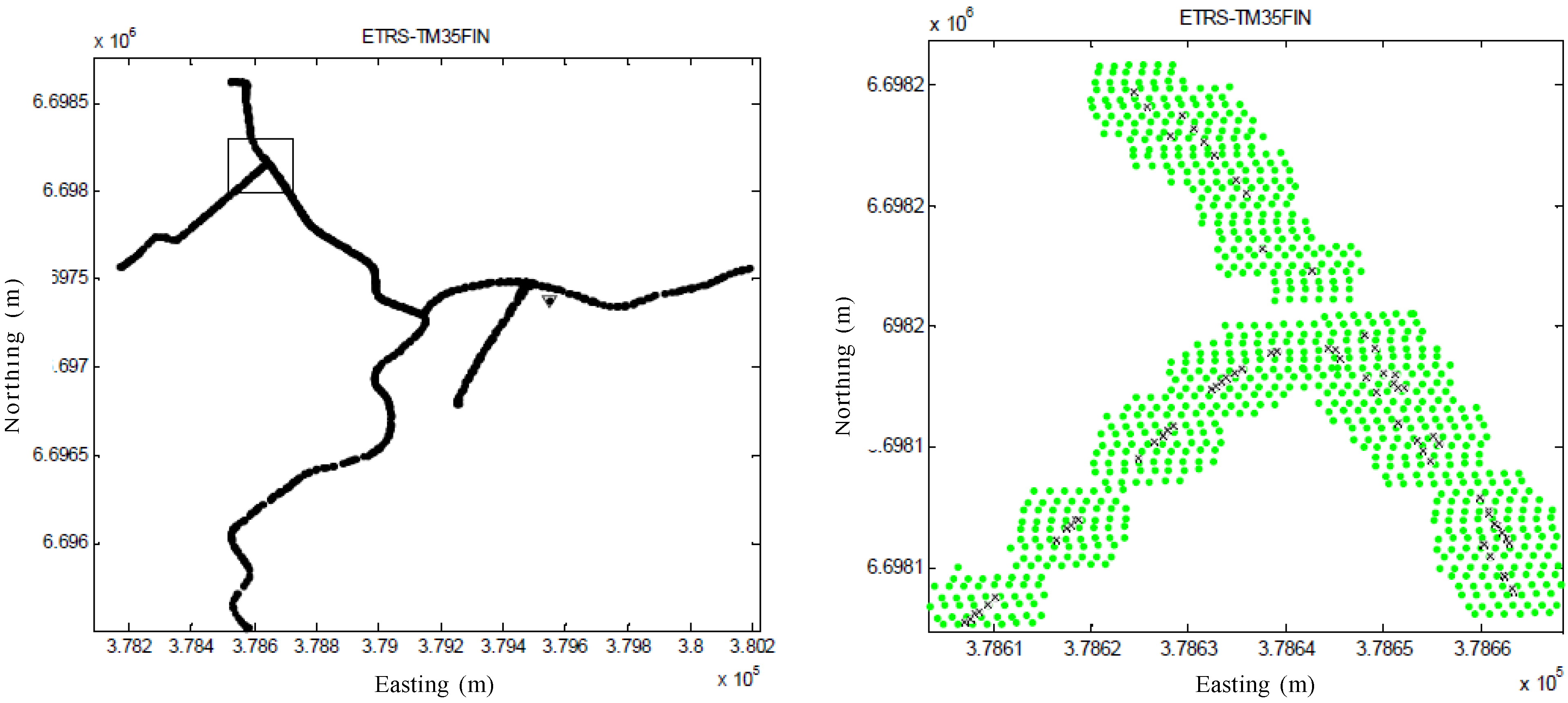
Real-time kinematic (RTK) GPS observations along the test area roads. Left: The complete test area. The RTK reference station is marked with a triangle. Right: A detailed view from the test area; the location of the detailed view is marked with a square in the left image. GPS observations are illustrated with black crosses, and ALS points near GPS observations are represented by green dots.
Figure 4.
Real-time kinematic (RTK) GPS observations along the test area roads. Left: The complete test area. The RTK reference station is marked with a triangle. Right: A detailed view from the test area; the location of the detailed view is marked with a square in the left image. GPS observations are illustrated with black crosses, and ALS points near GPS observations are represented by green dots.
During GPS data acquisition, measurements were collected using the “fixed” mode. In the “fixed” mode, the GPS delivers centimeter-level positioning precision if the integer estimate of the ambiguity search succeeds. The speed of the vehicle was maintained at approximately 30 km/h to achieve the desired point density. When the receiver dropped out of “fixed” mode, the vehicle was stopped until “on-the-fly” (OTF) re-initialization was achieved. This type of difficulty occurred only for VRS measurements, and the test area was measured twice using VRS. However, the busiest road was not measured with VRS GPS because it was not safe to stop the vehicle to wait for re-initialization. Using RTK, the complete test area was measured once without stops. A total of 1,589 points were collected using the base station (RTK) mode, and 2,183 points were collected using VRS mode; each set of data points corresponds to a driving distance of about 15 km.
3.3. Comparison of Laser Point Clouds and GPS Observations
Both laser scanning and GPS devices create 3D point clouds. These data sets have practically no points that exactly correspond with each other. Therefore, we interpolated ALS points to achieve better correspondence with GPS points. The interpolation method (
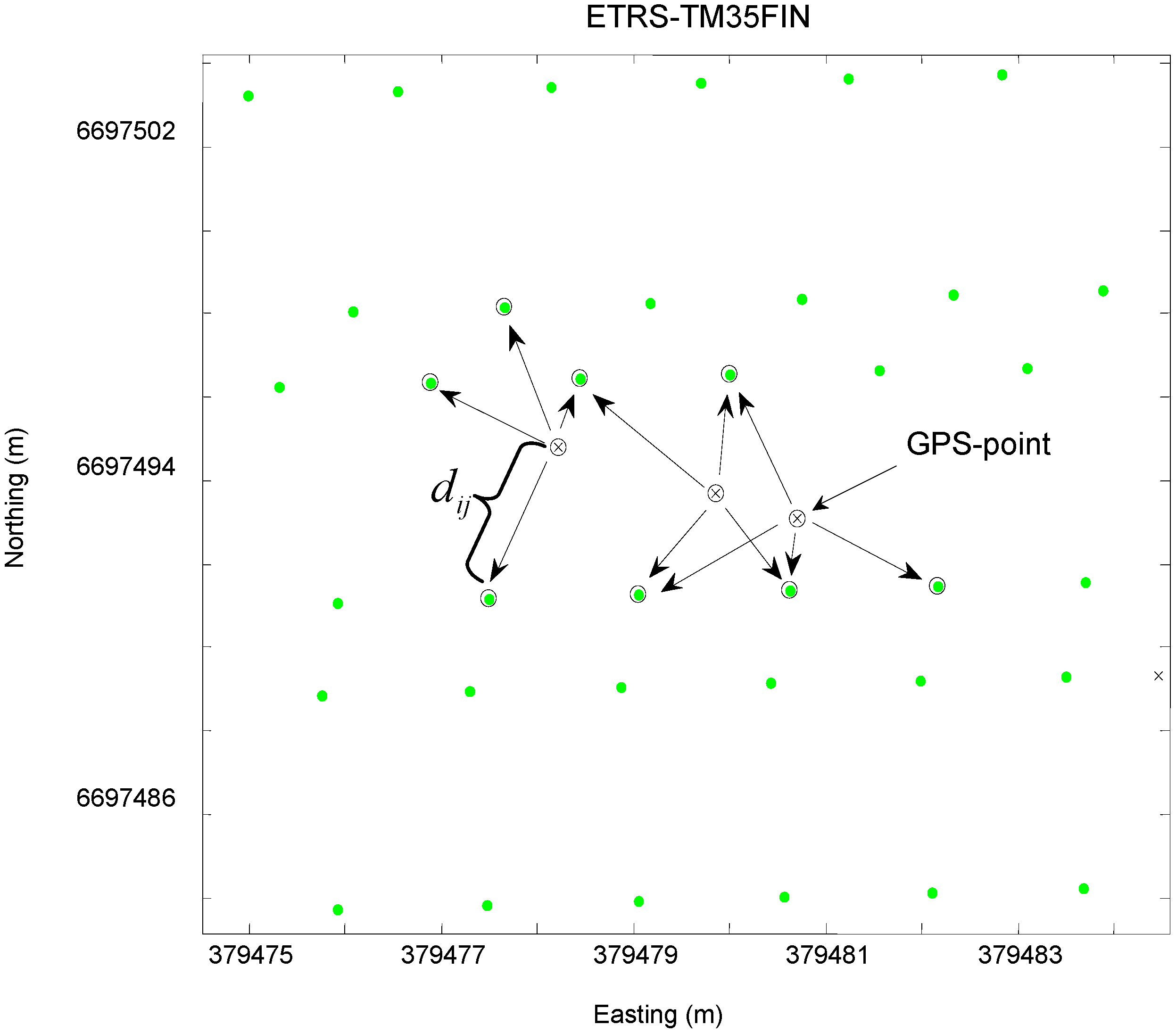
Figure 5) utilized weighted averages based on the distances from the four nearest ALS points (Equation (1)):
where
is the height of an interpolated ALS point to which we compare the GPS height,
are the heights of nearby ALS points, and
are the distances between GPS and ALS points.
N is the number of laser points used, and
i and
j are the GPS point and ALS point indices, respectively.
Figure 5.
Interpolation using four ALS points (green) to attain points corresponding with GPS observations.
Figure 5.
Interpolation using four ALS points (green) to attain points corresponding with GPS observations.
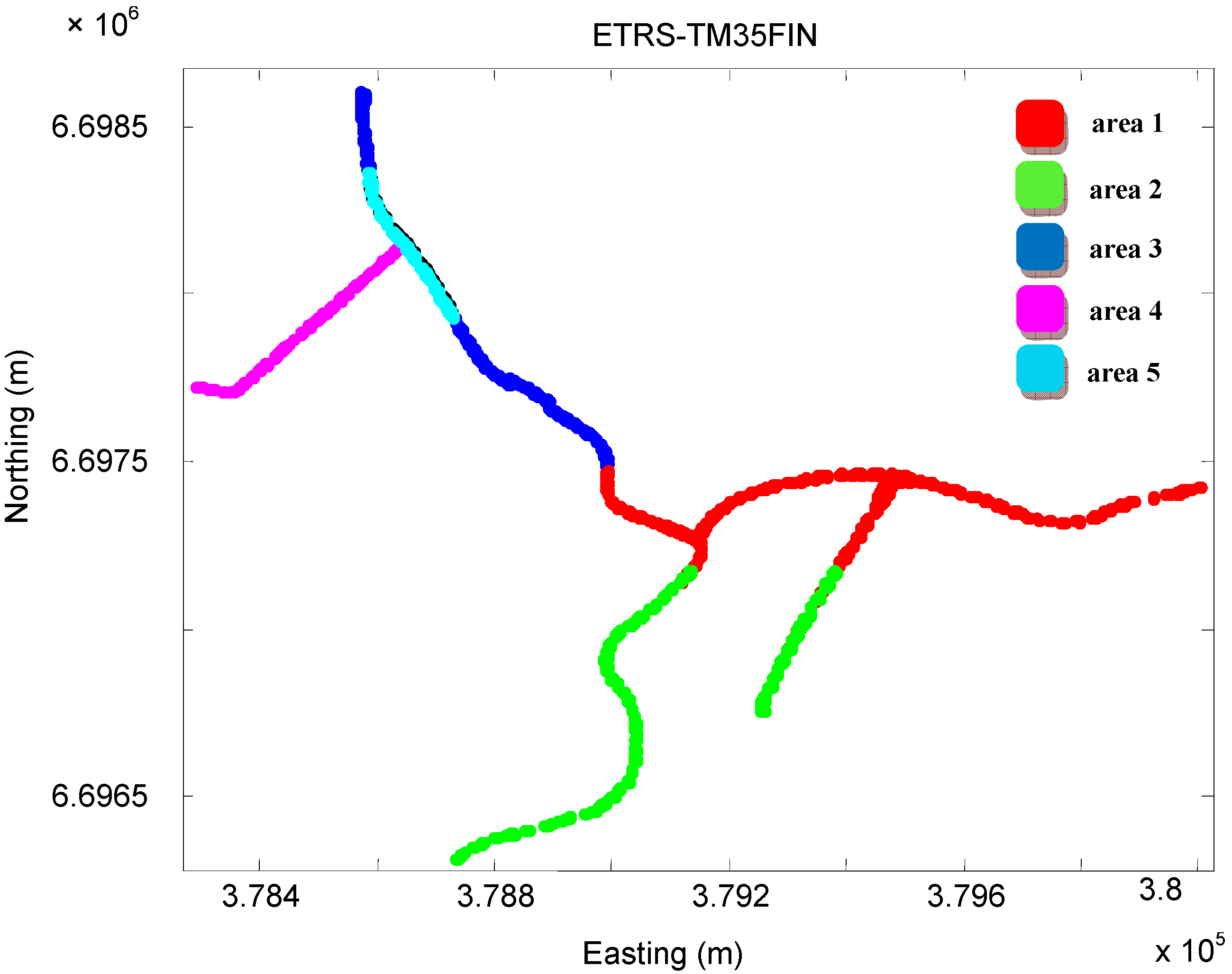
The test area was also divided into five sub-areas for more detailed examination (
Figure 6). Only sub-areas four and five had excellent satellite visibility. In areas one, two and three, trees and buildings occasionally reduced satellite visibility. Particularly in the case of VRS GPS measurements, these visibility obstacles caused a few gaps in data collection when the receiver dropped out.
Figure 6.
ALS data were evaluated within five sub-areas due to their different characteristics.
Figure 6.
ALS data were evaluated within five sub-areas due to their different characteristics.
4. Results and Discussion
Overall, when RTK and VRS measurements were compared with ALS points, the results were notably similar (
Table 1). Comparisons of the results of each measurement mode to ALS suggest that the overall shift between the data sets was −2.4 cm. The identical mean results were surprising because other researchers have indicated that reproducible 1.5–3.5 cm GPS height accuracies are obtainable (e.g., [
19]). In our test case, VRS measurements exhibited more deviation than did RTK-derived measurements and thus also included larger gross errors.
Table 1.
Overall height differences of interpolated laser points and GPS observations.
Table 1.
Overall height differences of interpolated laser points and GPS observations.
| Interpolation | | Height differences (cm) |
|---|
| No. of pts | Mean | Dispersion | Max. | Min. |
|---|
| RTK–ALS | 1,589 | −2.4 | ±4.5 | 30.1 | −35.9 |
| VRS–ALS | 2,183 | −2.4 | ±5.9 | 36.4 | −41.4 |
In
Table 2 and
Table 3, each sub-area is examined separately for RTK and VRS modes, respectively, and both similarities and differences between sub-areas are observed. For areas one and four the mean differences between the methods are similar. Satellite visibility in these areas was adequate, providing good satellite geometry and accuracy. For area five, the results from both methods were similar. However, the results from areas two and three had noticeable differences; these areas also exhibited the largest standard deviations, indicating that the accuracy of the GPS measurements was reduced. The high level of agreement between RTK and VRS observations is also illustrated in
Figure 7; in this figure, only the corresponding points that had a distance of 30 cm or less were included. Therefore, some gaps are visible in areas where driving trajectories differ by more than 30 cm.
Table 2.
Height differences between RTK GPS observations and interpolated laser points.
Table 2.
Height differences between RTK GPS observations and interpolated laser points.
| Test area | No. of RTK pts | Height differences (cm) |
|---|
| Mean | Dispersion | Max. | Min. |
|---|
| Area 1 | 630 | −4.0 | ±3.8 | 11.4 | −24.3 |
| Area 2 | 340 | −4.0 | ±5.5 | 8.5 | −35.9 |
| Area 3 | 311 | −1.1 | ±3.9 | 30.1 | −23.0 |
| Area 4 | 162 | 2.4 | ±3.8 | 20.0 | −9.5 |
| Area 5 | 146 | 0.6 | ±2.0 | 6.7 | −4.8 |
Table 3.
Height differences between VRS GPS observations and interpolated laser points.
Table 3.
Height differences between VRS GPS observations and interpolated laser points.
| Test area | No. of VRS pts | Height differences (cm) |
|---|
| Mean | Dispersion | Max | Min |
|---|
| Area 1 | 761 | −4.0 | ±4.5 | 29.5 | −22.6 |
| Area 2 | 363 | −5.5 | ±5.2 | 14.4 | −32.3 |
| Area 3 | 458 | −2.9 | ±7.6 | 36.4 | −41.4 |
| Area 4 | 365 | 2.4 | ±4.0 | 13.7 | −9.5 |
| Area 5 | 236 | 1.0 | ±3.9 | 11.1 | −20.3 |
Figure 7.
Visualization of height differences between VRS GPS and RTK GPS measurements. Points were included only when the distance between corresponding points was less than 30 cm.
Figure 7.
Visualization of height differences between VRS GPS and RTK GPS measurements. Points were included only when the distance between corresponding points was less than 30 cm.
If only numerical values are considered, the results may indicate that a slight rotational difference exists between ALS data and GPS observations. Areas one and two have negative height differences, whereas areas four and five, which are located on the opposite side of the test area, have positive values. However, this straightforward conclusion is not necessarily the correct one.
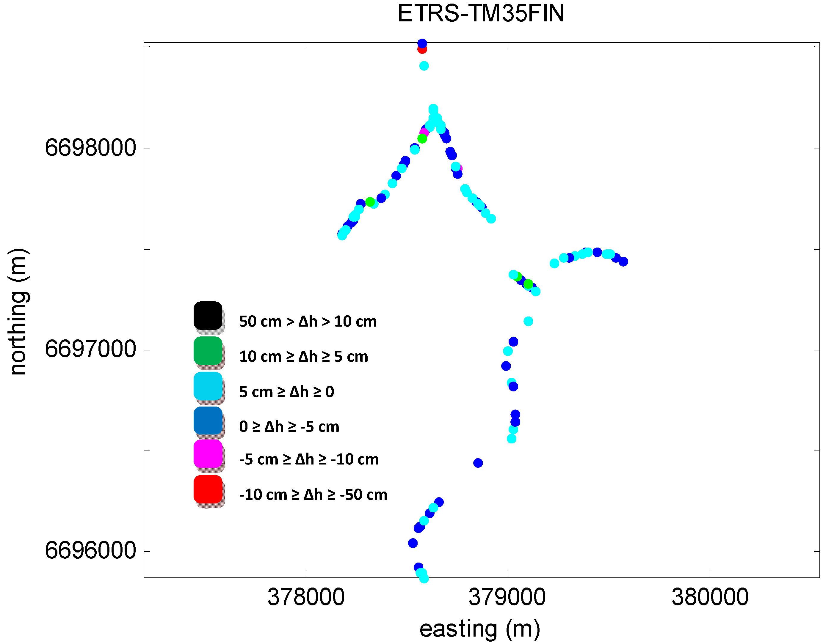
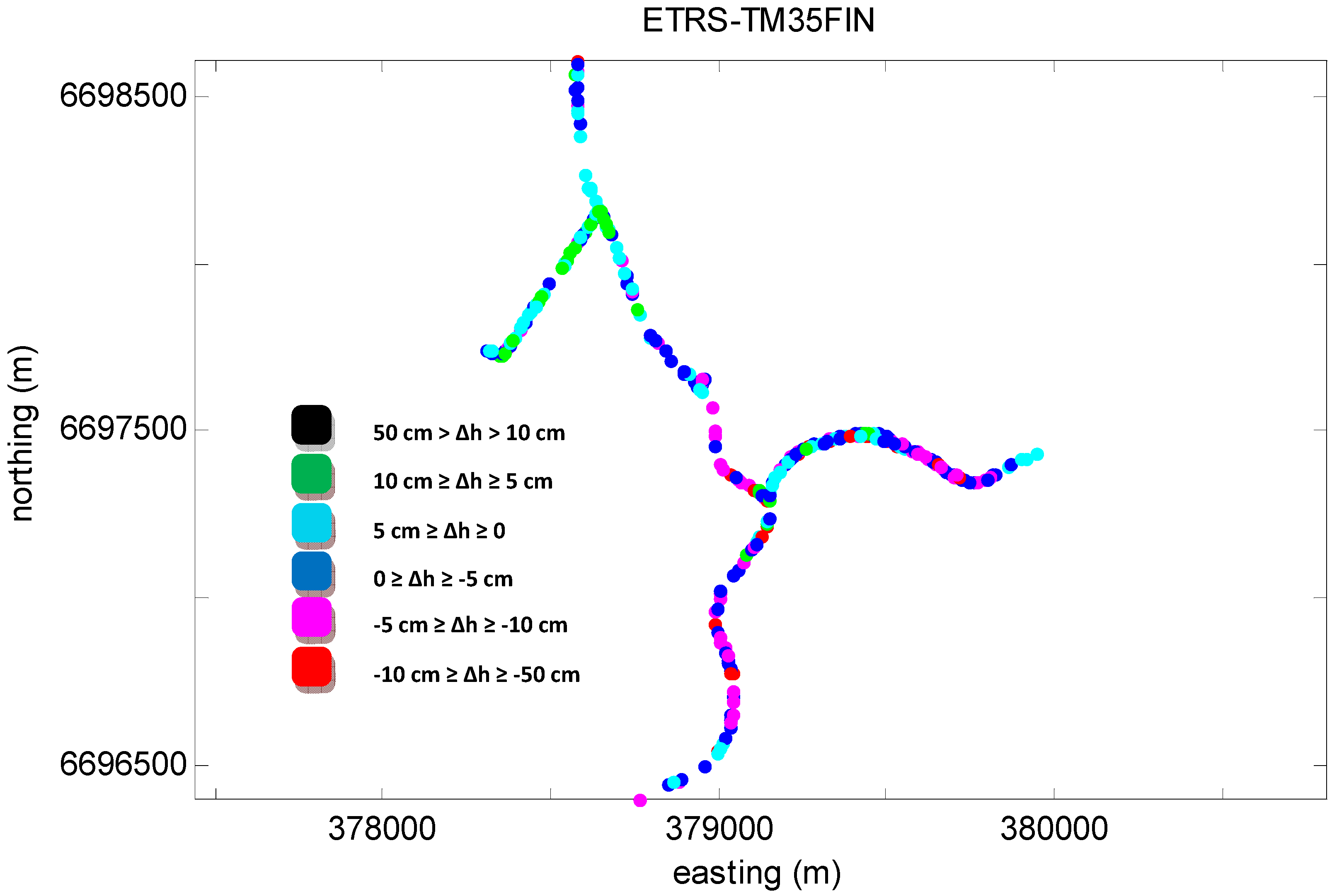
Figure 8 illustrates the distribution of height differences between RTK GPS measurements and interpolated ALS points, and
Figure 9 illustrates the corresponding case of VRS GPS observations and interpolated ALS points. However, there is no clear pattern that confirms a possible rotation although the noise increases in some parts of the test area. The largest dispersions in the sub-areas were ±5.5 cm in the case of RTK GPS and ±7.6 cm in the case of VRS GPS. In this case, the ALS data was well prepared, georeferenced and of good quality. Therefore, our analysis did not reveal significant need to correct the data when the final product, a DTM with an accuracy of 30 cm, was considered. The analysis also demonstrated that mobile vehicle-based GPS measurements along the road network can be used to evaluate the correctness of ALS point cloud heights. The expected accuracy of GPS in the vertical direction is close to 2 cm when measurement conditions are good, which limits the evaluation accuracy.
Figure 8.
Visualization of height differences between RTK GPS measurements and interpolated ALS points.
Figure 8.
Visualization of height differences between RTK GPS measurements and interpolated ALS points.
There are several advantages of using the methods described in this study: GPS data acquisition is relatively easy to perform, the road networks are easily accessible, the instrumentation is relatively inexpensive, the GPS systems can be rapidly set up, and these systems produce a considerable amount of reference information. The numerous observations permit robust comparisons and provide information about possible internal problems with ALS data. Therefore, this method provides a feasible alternative to current methods for collecting ground control data. Currently, ground control data is principally collected via manual measurements of several relatively small control areas using either GPS or tacheometer. Our method requires the presence of an even distribution of roads within the campaign area, which may be an obstacle to obtaining sufficient information in some remote areas. In addition, satellite visibility may be an obstacle to obtaining sufficient information in urban areas or dense forests. A single GPS measurement can include errors; based on satellite geometry conditions, erroneous observations can sometimes be detected. However, in the case of mobile GPS measurements, repeating measurement trajectories can yield valuable information about their accuracy.
Figure 9.
Visualization of height differences between VRS GPS measurements and interpolated ALS points.
Figure 9.
Visualization of height differences between VRS GPS measurements and interpolated ALS points.
5. Conclusions
We tested the use of vehicle-mounted RTK and VRS GPS positioning for the evaluation of the correctness of ALS data. The road network in the test area was measured with both vehicle-based GPS equipment and ALS. When the complete test area was included, the mean height difference between ALS data and GPS observations was −2.4 cm, and the same result was achieved using either RTK or VRS measurement methods. However, an examination of sub-areas based on the characteristics of the environment in the test area revealed that some variations existed between the methods. Generally, VRS GPS data exhibited slightly more dispersion than RTK GPS data. These discrepancies were distributed evenly over the test area, and, therefore, we were not able to detect any significant rotation between ALS data and GPS observations.
The maximum difference of the mean error between RTK- and VRS-based comparisons within a single sub-area was 1.8 cm (Test area three). In this sub-area, satellite visibility problems caused gaps in acquired data, especially for VRS GPS. In the best cases (Test areas one and four), the mean difference between the two GPS measurement methods was zero. It can be concluded that satellite visibility is one of the main concerns affecting accuracy when GPS observations are used as reference data. The positioning accuracy of a vehicle is known to be improved when GPS devices are used in conjunction with IMU and odometers; however, IMU is notably expensive. In our test setup, only GPS receivers were included. Our method has the advantages of using a relatively inexpensive system, easy access to the road network, rapid setup, and the amount of generated data. In areas having non-optimal satellite visibility, redundant observations are recommended. This redundancy can be achieved by revisiting known benchmarks or measuring the same roads repeatedly.
In our test case, the reference measurements using either RTK or VRS GPS were sufficiently accurate for the evaluation of the correctness of ALS data heights. The vertical accuracy requirement for ALS data is 30 cm; according to our analysis, this accuracy requirement was fulfilled well.


