Consequences of Uncertainty in Global-Scale Land Cover Maps for Mapping Ecosystem Functions: An Analysis of Pollination Efficiency

Abstract
:1. Introduction
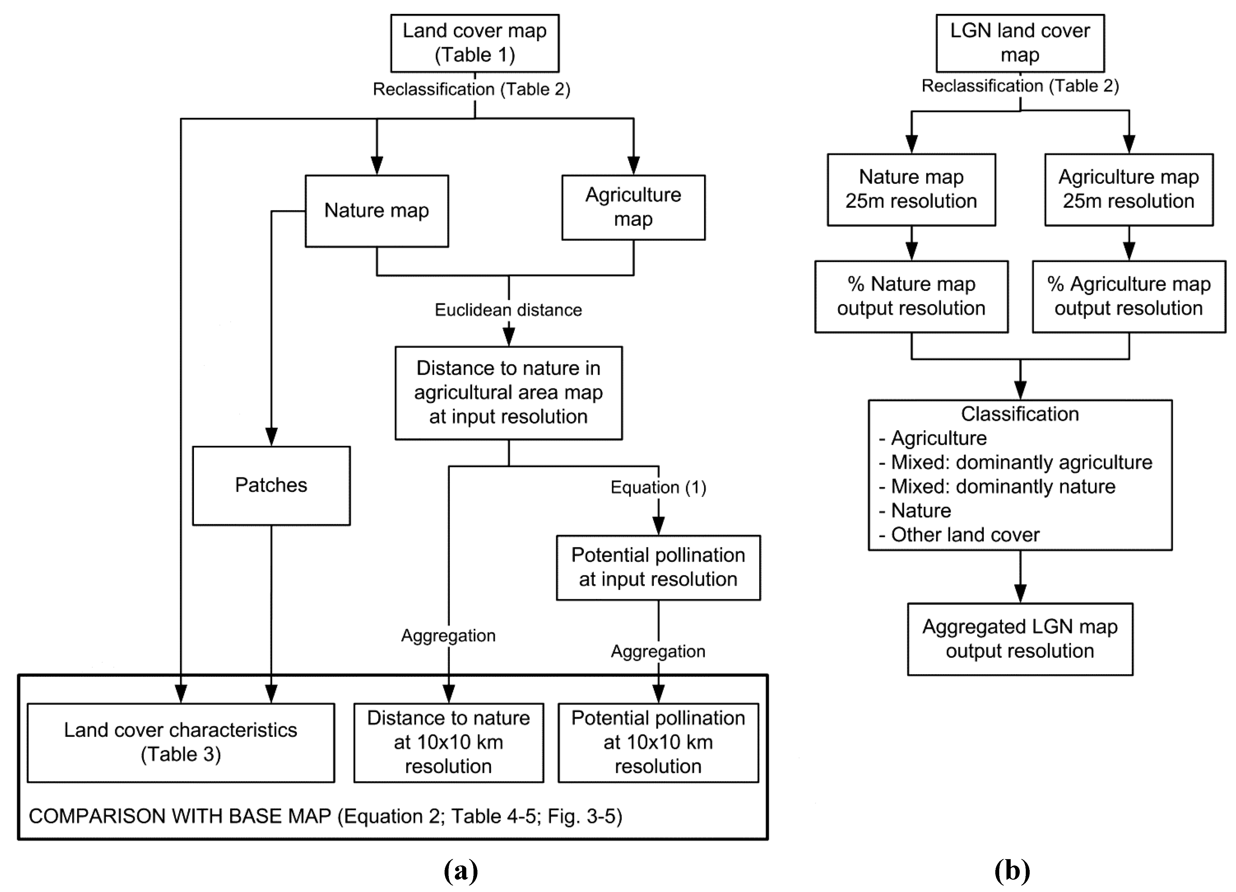
2. Methods
2.1. Case Study

| Name | Resolution (m) | Extent | Satellite data source | Year of data acquisition | # categories * | Remarks | Reference |
|---|---|---|---|---|---|---|---|
| LGN | 25 | Netherlands | Landsat, IRS-LII, ERS-SAR radar. | 2003–2004 | 39 | Use and cover. | [36] |
| CORINE | 100 | Europe | Landsat/SPOT | 2000 | 29 | Use and cover. Mostly dominant classes. | [37] |
| Glob Cover | 252 | Global | ENVISAT/MERIS | 2004–2006 | 15 | Cover. Many mixed classes. | [38] |
| GLC2000 | 825 | Global | SPOT4 VEGETATION | 1999–2000 | 8 | Cover. Some mixed classes. | [19] |
| PELCOM | 1,100 | Europe | NOAA-AVHRR, MARS | 1999 | 10 | Cover. Dominant classes only. | [18] |

2.2. Land Cover Data
| Main land cover type | LGN | CORINE | GlobCover | GLC2000 | PELCOM |
|---|---|---|---|---|---|
| Agriculture | Grassland; Maize; Potatoes; Sugar beets; Cereals; Other crops; Orchards; Flower bulbs; Fen meadow areas. | Non-irrigated arable land; Fruit and berry plantations; Pastures; Complex cultivation patterns. | Rainfed croplands; Closed-open grassland. | Herbaceous cover, closed-open; Cultivated and managed areas. | Grassland; Non-irrigated arable land. |
| Mixed | - | Land principally occupied by agriculture, with significant areas of natural vegetation (50). | Mosaic cropland-grassland-shrubland-forest (40); Mosaic forest-shrubland-grassland (60); Mosaic grassland-forest-shrubland (40). | Mosaic: Cropland/Shrub or Grass Cover (50). | - |
| Nature | Deciduous/coniferous forests, inside/outside urban area with high housing density; Marshes; Open/closed dune vegetation; Open drift sands; Heathland in dunes with no/some/strong invasion of grasses;Peat moors; Forest on peat moors; Other swamp vegetation; Reedlands; Forest in swamps; Other open natural vegetation; Bare soil in nature areas. | Green urban areas; Broad-leaved/Coniferous/Mixed forest; Natural grasslands; Moors and heathland; Transitional woodland-shrub; Beaches, dunes, sands; Inland marshes; Peat bogs; Salt marshes. | Forest: closed broadleaved deciduous; Closed needleleaved evergreen; Open needleleaved deciduous or evergreen; Closed to open mixed broadleaved and needleleaved; Sparse vegetation; Closed-open vegetation on regularly flooded waterlogged soil. | Tree Cover: broadleaved, deciduous, closed; needle-leaved, evergreen; mixed leaf type. | Coniferous/deciduous/mixed forest; Wetlands. |
| Other | Greenhouses; Fresh/saline water; Built-up urban/rural/agricultural; Grassland in urban area; Bare soil in built-up rural areas; Major roads and railroads. | Urban fabric continuous/discontinuous; Industrial/commercial units; Roads and railroads; Ports; Airports; Mineral extraction sites; Dump sites; Construction sites; Sport/leisure facilities; Intertidal flats; Water; Estuaries. | Artificial surfaces; Bare areas; Water bodies. | Water bodies Artificial surfaces. | Inland waters; Sea; urban areas. |
2.3. Mapping of Ecosystem Properties and Functions
2.4. Analyses
3. Results
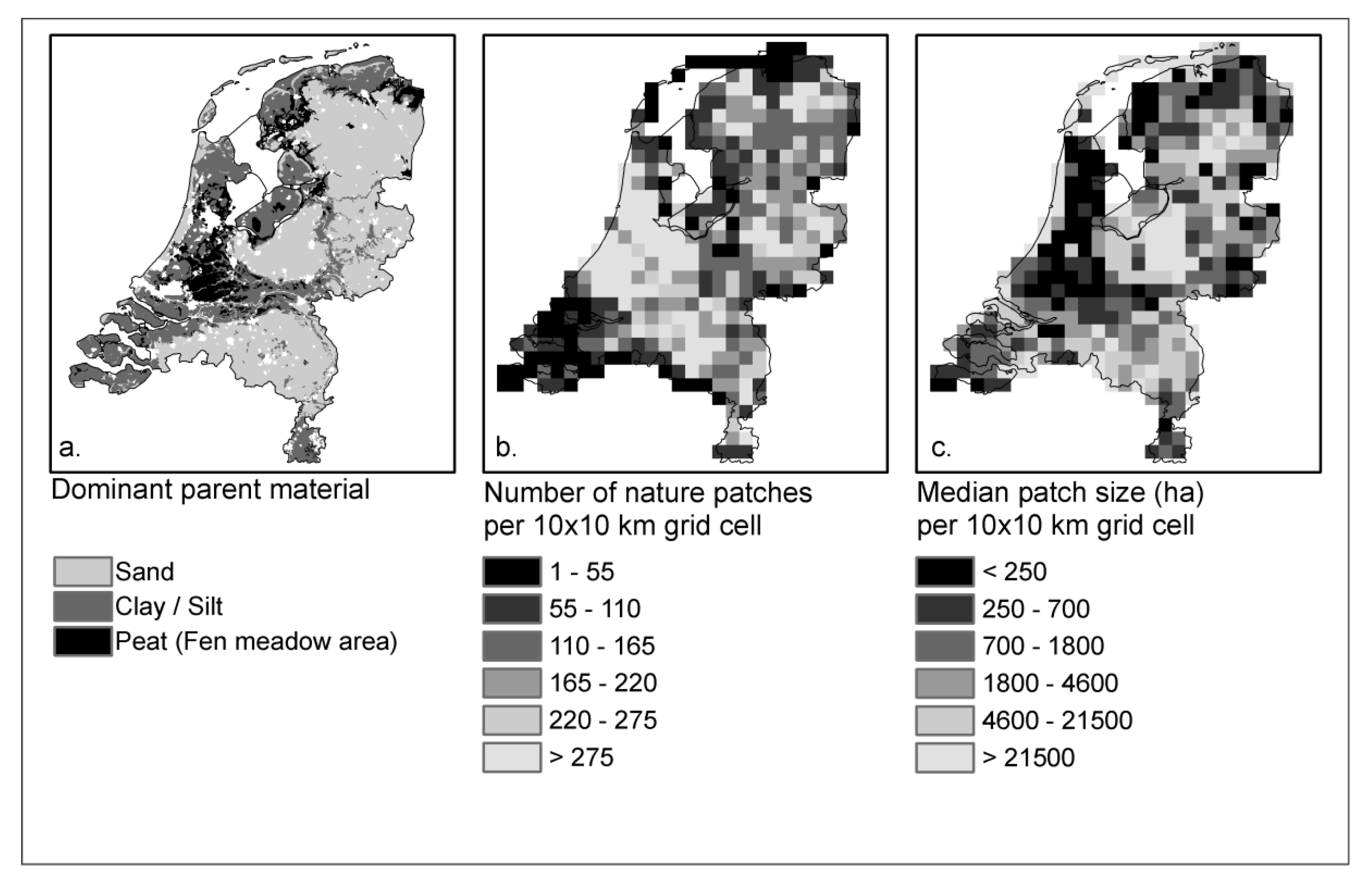
3.1. Land Cover Characteristics
| Map/Resolution | Land cover area (%) | Number of nature patches | Median patch size (ha) | Mean (StDev) Dnature (m) | Mean (StDev) YRF (%) | |||||||
|---|---|---|---|---|---|---|---|---|---|---|---|---|
| Agriculture | Nature | Mixed | Other | |||||||||
| LGN | 52% | 14% | 0% | 34% | 77,931 | 0.3 | 538 | (262) | 63 | (11) | ||
| Aggregated LGN maps | ||||||||||||
| 100 m | 52% | 12% | 1% | 35% | 33,574 | 1.0 | 696 | (353) | 59 | (11) | ||
| 250 m | 53% | 10% | 2% | 34% | 5,397 | 12.5 | 943 | (419) | 54 | (10) | ||
| 825 m | 53% | 8% | 5% | 34% | 838 | 136.1 | 1,723 | (854) | 48 | (10) | ||
| 1,100 m | 52% | 8% | 6% | 34% | 601 | 200.0 | 1,928 | (960) | 47 | (10) | ||
| Real land cover maps | ||||||||||||
| CORINE | 58% | 17% | 3% | 23% | 1,489 | 65.0 | 1,824 | (1,450) | 50 | (11) | ||
| GLOBCOVER | 45% | 23% | 7% | 25% | 2,558 | 19.1 | 416 | (177) | 69 | (7) | ||
| GLC2000 | 72% | 6% | 0% | 22% | 647 | 136.1 | 3,580 | (1,995) | 41 | (4) | ||
| PELCOM | 71% | 5% | 0% | 24% | 316 | 200.0 | 4,088 | (2,156) | 40 | (4) | ||

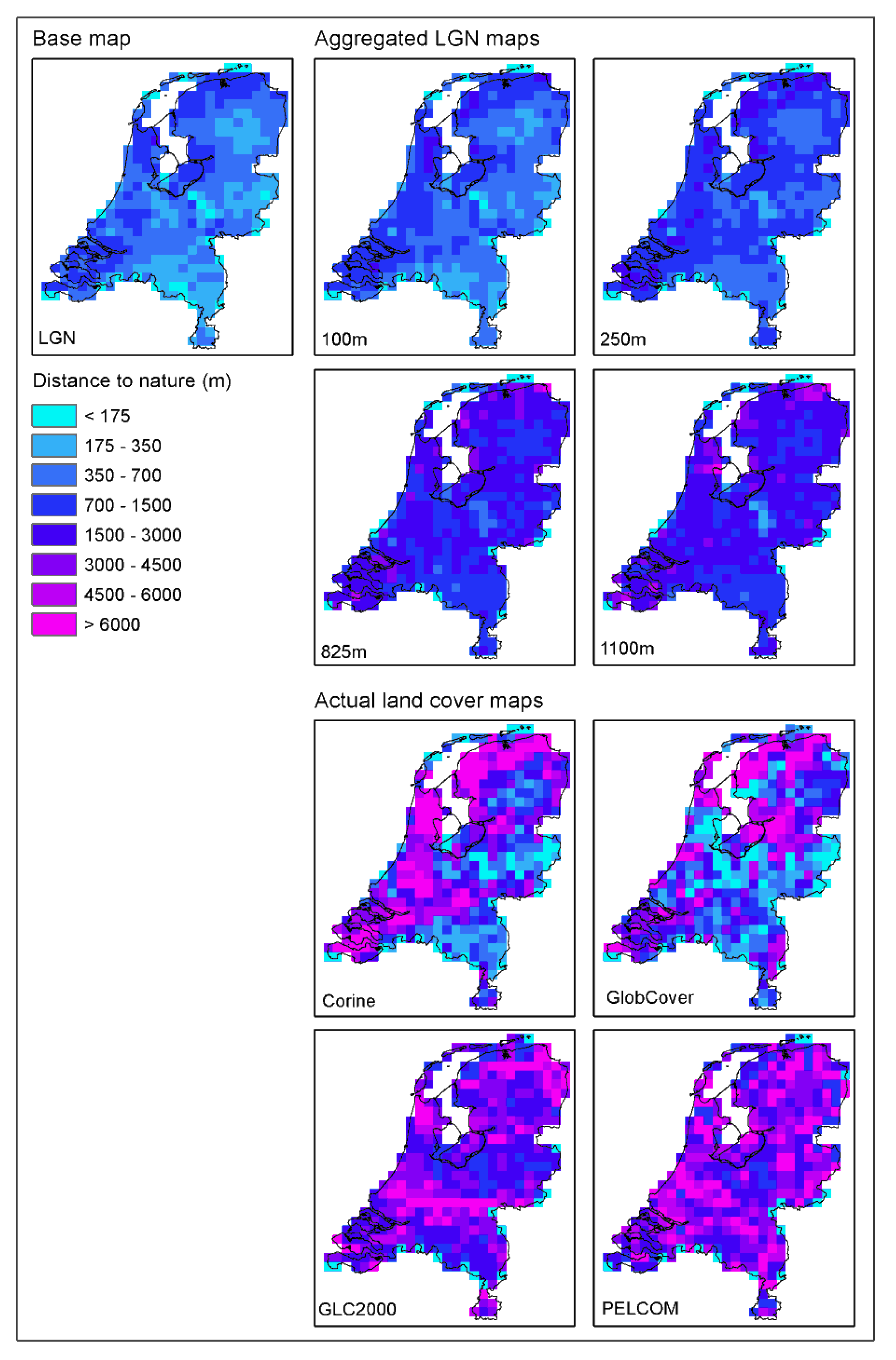
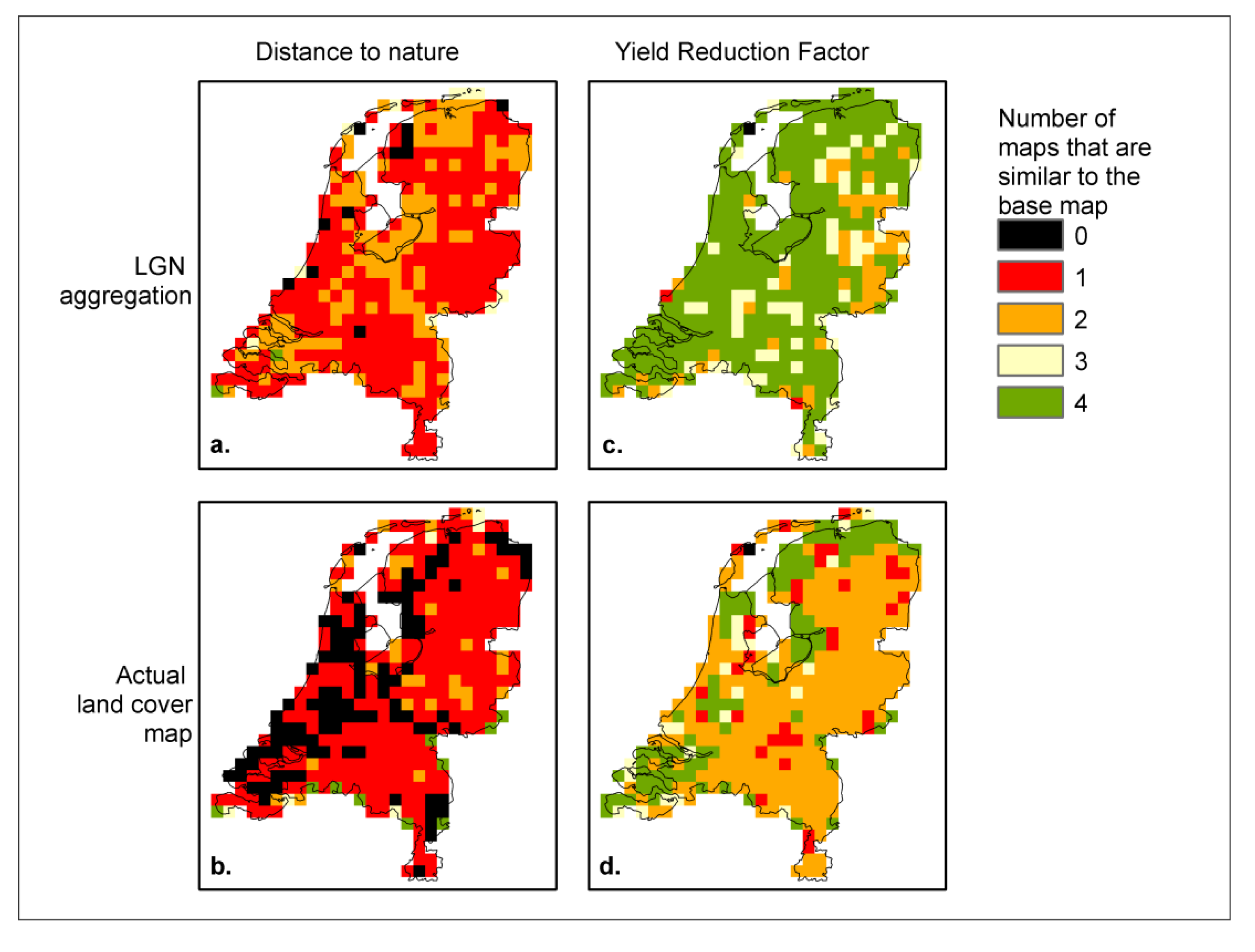
3.2. Distance to Nature in Agricultural Areas
| Map/Resolution | Similarity with the base map | ||
|---|---|---|---|
| Dnature | YRF | ||
| Aggregated LGN maps | |||
| 100 m | 0.78 | 0.94 | |
| 250 m | 0.57 | 0.86 | |
| 825 m | 0.33 | 0.77 | |
| 1,100 m | 0.30 | 0.76 | |
| Real land cover maps | |||
| CORINE | 0.38 | 0.80 | |
| GLOBCOVER | 0.69 | 0.89 | |
| GLC2000 | 0.18 | 0.65 | |
| PELCOM | 0.18 | 0.63 | |


| Resolution | Maps | Dnature | YRF |
|---|---|---|---|
| 100 m | CORINE–LGN100 | 0.47 | 0.85 |
| 250 m | GLOBCOVER–LGN250 | 0.47 | 0.79 |
| 825 m | GLC2000–LGN825 | 0.51 | 0.84 |
| 1,000 m | PELCOM–LGN1100 | 0.46 | 0.83 |
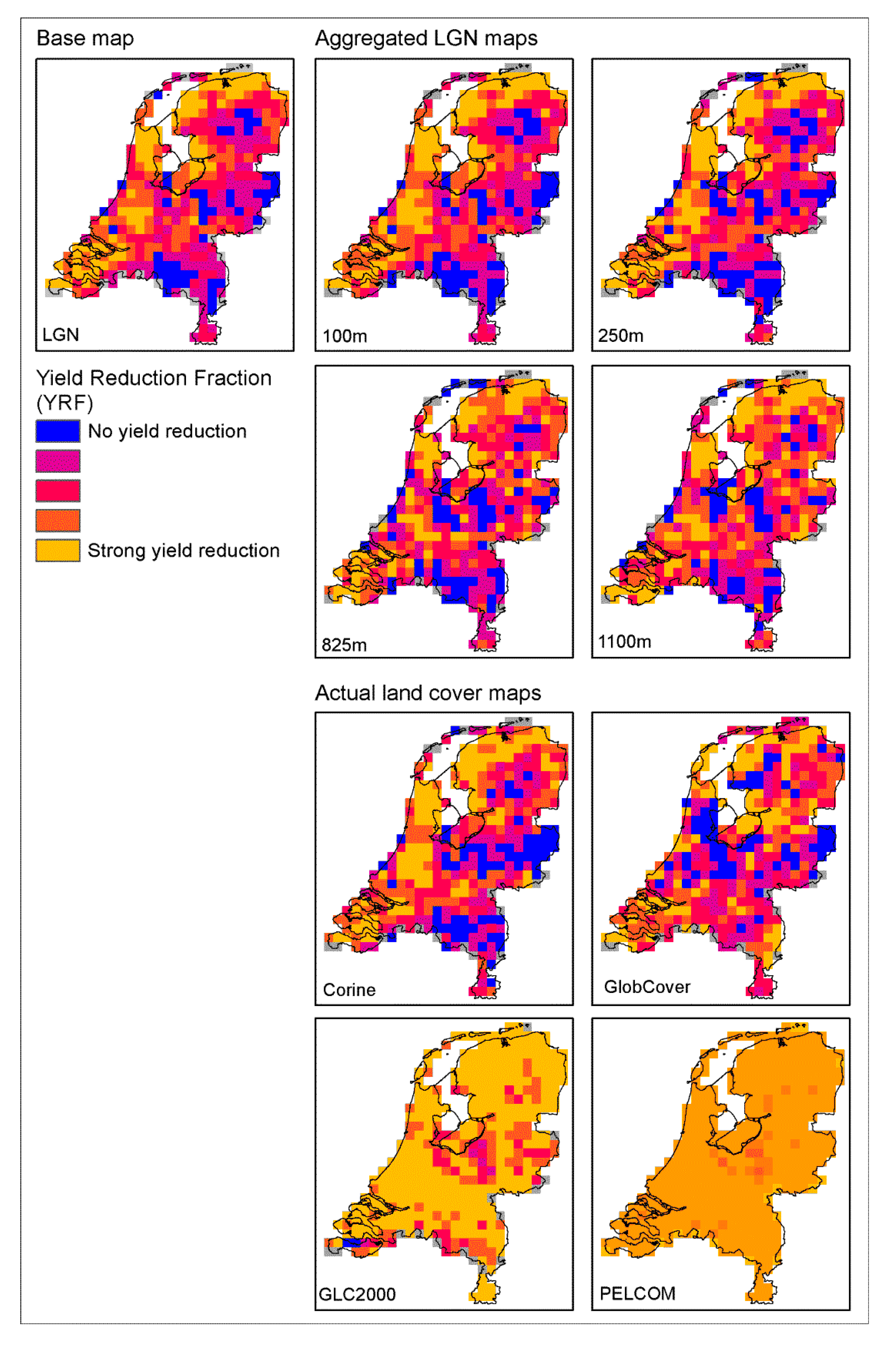
3.3. Yield Reduction Fraction

4. Discussion
4.1. Effects of Resolution
4.2. Effects of Satellite Imagery Resolution and Classification
4.3. Methodological Issues
4.4. Consequences for Mapping Ecosystem Services at a Global Scale
5. Conclusions and Recommendations
References
- Millennium Ecosystem Assessment (MA). Ecosystems and Human Well-Being: Synthesis; Island Press: Washington, DC, USA, 2005. [Google Scholar]
- TEEB. The Economics of Ecosystems and Biodiversity for National and International Policy Makers—Summary: Responding to the Value of Nature 2009; The Economics of Ecosystems and Biodiversity: Nairobi, Kenya, 2009. [Google Scholar]
- European Commission. The CAP towards 2020: Meeting the Food, Natural Resource and Territorial Challenges of the Future; Communication from the Commission to the Council, the European Parliament, the European Economic and Social Committee and the Committee of the Regions; European Commission: Brussel, Belgium, 18 November 2010. [Google Scholar]
- Wischmeyer, W.H.; Smith, D.D. Predicting Rainfall Erosion Losses: A Guide to Conservation Planning; US Department of Agriculture: Washington, DC, USA, 1978; Volume 537, p. 69. [Google Scholar]
- Follain, S.; Walter, C.; Bonté, P.; Marguerie, D.; Lefevre, I. A-horizon dynamics in a historical hedged landscape. Geoderma 2009, 150, 334–343. [Google Scholar] [CrossRef]
- Fohrer, N.; Haverkamp, S.; Frede, H.G. Assessment of the effects of land use patterns on hydrologic landscape functions: Development of sustainable land use concepts for low mountain range areas. Hydrol. Process. 2005, 19, 659–672. [Google Scholar] [CrossRef]
- Johnston, C.A.; Detenbeck, N.E.; Niemi, G.J. The cumulative effect of wetlands on stream water quality and quantity. A landscape approach. Biogeochemistry 1990, 10, 105–141. [Google Scholar] [CrossRef]
- Ricci, B.; Franck, P.; Toubon, J.-F.; Bouvier, J.-C.; Sauphanor, B.; Lavigne, C. The influence of landscape on insect pest dynamics: A case study in southeastern France. Landsc. Ecol. 2009, 24, 337–349. [Google Scholar] [CrossRef]
- Willemen, L.; Verburg, P.H.; Hein, L.; van Mensvoort, M.E.F. Spatial characterization of landscape functions. Landsc. Urban Plan. 2008, 88, 34–43. [Google Scholar] [CrossRef]
- Fyhri, A.; Jacobsen, J.K.S.; Tømmervik, H. Tourists’ landscape perceptions and preferences in a Scandinavian coastal region. Landsc. Urban Plan. 2009, 91, 202–211. [Google Scholar] [CrossRef]
- O’Farrell, P.; Reyers, B.; Le Maitre, D.; Milton, S.; Egoh, B.; Maherry, A.; Colvin, C.; Atkinson, D.; de Lange, W.; Blignaut, J.; et al. Multi-functional landscapes in semi-arid environments: Implications for biodiversity and ecosystem services. Landsc. Ecol. 2010, 25, 1231–1246. [Google Scholar] [CrossRef]
- Anderson, B.J.; Armsworth, P.R.; Eigenbrod, F.; Thomas, C.D.; Gillings, S.; Heinemeyer, A.; Roy, D.B.; Gaston, K.J. Spatial covariance between biodiversity and other ecosystem service priorities. J. Appl. Ecol. 2009, 46, 888–896. [Google Scholar] [CrossRef]
- Chen, N.; Li, H.; Wang, L. A GIS-based approach for mapping direct use value of ecosystem services at a county scale: Management implications. Ecol. Econ. 2009, 68, 2768–2776. [Google Scholar] [CrossRef]
- Alcamo, J.; van Vuuren, D.; Ringler, C.; Cramer, W.; Masui, T.; Alder, J.; Schulze, K. Changes in nature’s balance sheet: Model-based estimates of future worldwide ecosystem services. Ecol. Soc. 2005, 10. art. 19. [Google Scholar]
- Naidoo, R.; Balmford, A.; Costanza, R.; Fisher, B.; Green, R.E.; Lehner, B.; Malcolm, T.R.; Ricketts, T.H. Global mapping of ecosystem services and conservation priorities. Proc. Nat. Acad. Sci. USA 2008, 105, 9495–9500. [Google Scholar] [CrossRef] [PubMed]
- De Groot, R.S.; Alkemade, R.; Braat, L.; Hein, L.; Willemen, L. Challenges in integrating the concept of ecosystem services and values in landscape planning, management and decision making. Ecol. Complex. 2010, 7, 260–272. [Google Scholar] [CrossRef]
- Nol, L.; Verburg, P.H.; Heuvelink, G.B.M.; Molenaar, K. Effect of land cover data on nitrous oxide inventory in fen meadows. J. Environ. Qual. 2008, 37, 1209–1219. [Google Scholar] [CrossRef] [PubMed]
- Mucher, C.A.; Steinnocher, K.T.; Kressler, F.P.; Heunks, C. Land cover characterization and change detection for environmental monitoring of pan-Europe. Int. J. Remote Sens. 2000, 21, 1159–1181. [Google Scholar] [CrossRef]
- Bartholomé, E.; Belward, A.S. GLC2000: A new approach to global land cover mapping from Earth observation data. Int. J. Remote Sens. 2005, 26, 1959–1977. [Google Scholar] [CrossRef]
- Ozdogan, M.; Woodcock, C.E. Resolution dependent errors in remote sensing of cultivated areas. Remote Sens. Environ. 2006, 103, 203–217. [Google Scholar] [CrossRef]
- Herold, M.; Mayaux, P.; Woodcock, C.E.; Baccini, A.; Schmullius, C. Some challenges in global land cover mapping: An assessment of agreement and accuracy in existing 1 km datasets. Remote Sens. Environ. 2008, 112, 2538–2556. [Google Scholar] [CrossRef]
- Clevers, J.G.P.W.; Schaepman, M.E.; Mücher, C.A.; de Wit, A.J.W.; Zurita-Milla, R.; Bartholomeus, H.M. Using MERIS on Envisat for land cover mapping in the Netherlands. Int. J. Remote Sens. 2007, 28, 637–652. [Google Scholar] [CrossRef] [Green Version]
- Fang, S.; Gertner, G.; Wang, G.; Anderson, A. The impact of misclassification in land use maps in the prediction of landscape dynamics. Landsc. Ecol. 2006, 21, 233–242. [Google Scholar] [CrossRef]
- Schulp, C.J.E.; Veldkamp, A. Long-term landscape—Land use interactions as explaining factor for soil organic matter variability in agricultural landscapes. Geoderma 2008, 146, 457–465. [Google Scholar] [CrossRef]
- Thies, C.; Steffan-Dewenter, I.; Tscharntke, T. Effects of landscape context on herbivory and parasitism at different spatial scales. Oikos 2003, 101, 18–25. [Google Scholar] [CrossRef]
- Schmit, C.; Rounsevell, M.D.A.; La Jeunesse, I. The limitations of spatial land use data in environmental analysis. Environ. Sci. Policy 2006, 9, 174–188. [Google Scholar] [CrossRef]
- Le Conte, Y.; Ellis, M.; Ritter, W. Varroa mites and honey bee health: Can Varroa explain part of the colony losses? Apidologie 2010, 41, 353–363. [Google Scholar] [CrossRef]
- Chacoff, N.P.; Aizen, M.A.; Aschero, V. Proximity to forest edge does not affect crop production despite pollen limitation. Proc. R. Soc. B 2008, 275, 907–913. [Google Scholar] [CrossRef] [PubMed]
- Klein, A.-M.; Vaissiere, B.E.; Cane, J.H.; Steffan-Dewenter, I.; Cunningham, S.A.; Kremen, C.; Tscharntke, T. Importance of pollinators in changing landscapes for world crops. Proc. R. Soc. B 2007, 274, 303–313. [Google Scholar] [CrossRef] [PubMed]
- Kleijn, D.; van Langevelde, F. Interacting effects of landscape context and habitat quality on flower visiting insects in agricultural landscapes. Basic Appl. Ecol. 2006, 7, 201–214. [Google Scholar] [CrossRef]
- Albrecht, M.; Duelli, P.; Muller, C.; Kleijn, D.; Schmid, B. The Swiss agri-environment scheme enhances pollinator diversity and plant reproductive success in nearby intensively managed farmland. J. Appl. Ecol. 2007, 44, 813–822. [Google Scholar] [CrossRef]
- Kohler, F.; Verhulst, J.; van Klink, R.; Kleijn, D. At what spatial scale do high-quality habitats enhance the diversity of forbs and pollinators in intensively farmed landscapes? J. Appl. Ecol. 2008, 45, 753–762. [Google Scholar] [CrossRef]
- Steffan-Dewenter, I.; Tscharntke, T. Effects of habitat isolation on pollinator communities and seed set. Oecologia 1999, 121, 432–440. [Google Scholar] [CrossRef]
- Ricketts, T.H.; Regetz, J.; Steffan-Dewenter, I.; Cunningham, S.A.; Kremen, C.; Bogdanski, A.; Gemmill-Herren, B.; Greenleaf, S.S.; Klein, A.M.; Mayfield, M.M.; Morandin, L.A.; Ochieng’, A.; Viana, B.F. Landscape effects on crop pollination services: Are there general patterns? Ecol. Lett. 2008, 11, 499–515. [Google Scholar] [CrossRef] [PubMed]
- Kremen, C.; Williams, N.M.; Bugg, R.L.; Fay, J.P.; Thorp, R.W. The area requirements of an ecosystem service: Crop pollination by native bee communities in California. Ecol. Lett. 2004, 7, 1109–1119. [Google Scholar] [CrossRef]
- Hazeu, G.W. Landelijk Grondgebruiksbestand Nederland (LGN5); Vervaardiging, nauwkeurigheid en gebruik; Report 1213; Alterra: Wageningen, The Netherlands, 2005; p. 92. [Google Scholar]
- Bossard, M.; Feranec, J.; Otahel, J. CORINE Land Cover Technical Guide—Addendum 2000; Technical Report No. 40; European Environment Agency: Copenhagen, Denmark, 2000; p. 105. [Google Scholar]
- Bicheron, P.; Defourny, P.; Brockmann, C.; Schouten, L.; Vancutsem, C.; Huc, M.; Bontemps, S.; Leroy, M.; Achard, F.; Herold, M.; et al. GlobCover: Products Description and Validation Report; Medias France: Toulouse, France, 2008. [Google Scholar]
- Gallai, N.; Salles, J.-M.; Settele, J.; Vaissière, B.E. Economic valuation of the vulnerability of world agriculture confronted with pollinator decline. Ecol. Econ. 2009, 68, 810–821. [Google Scholar] [CrossRef] [Green Version]
- Visser, H.; de Nijs, T. The map comparison kit. Environ. Model. Softw. 2006, 21, 346–358. [Google Scholar] [CrossRef]
- Hagen-Zanker, A. Comparing Contiuous Valued Raster Data. A Cross Disciplinary Literature Scan; Research Institute for Knowledge Systems: Maastricht, The Netherlands, 2006; p. 59. [Google Scholar]
- Gonzales, E.; Gergel, S. Testing assumptions of cost surface analysis—A tool for invasive species management. Landsc. Ecol. 2007, 22, 1155–1168. [Google Scholar] [CrossRef]
- Verburg, P.H.; Neumann, K.; Nol, L. Challenges in using land use and land cover data for global change studies. Glob. Change Biol. 2011, 17, 974–989. [Google Scholar] [CrossRef]
- Moody, A.; Woodcock, C.E. Calibration-based models for correction of area estimates derived from coarse resolution land-cover data. Remote Sens. Environ. 1996, 58, 225–241. [Google Scholar] [CrossRef]
- Gathmann, A.; Tscharntke, T. Foraging ranges of solitary bees. J. Anim. Ecol. 2002, 71, 757–764. [Google Scholar] [CrossRef]
- Neumann, K.; Herold, M.; Hartley, A.; Schmullius, C. Comparative assessment of CORINE2000 and GLC2000: Spatial analysis of land cover data for Europe. Int. J. Appl. Earth Obs. Geoinf. 2007, 9, 425–437. [Google Scholar] [CrossRef]
- EEA. CORINE Land Cover: Part 1: Methodology; CORINE Land Cover; Commission of the European Communities: Copenhagen, Denmark, 1994; Available online: http://www.eea.europa.eu/publications/COR0-landcover (accessed on 14 April 2011).
- Bakker, M.M.; Veldkamp, A. Modelling land change: The issue of use and cover in wide-scale applications. J. Land Use Sci. 2008, 3, 203–213. [Google Scholar] [CrossRef]
- Kaptué Tchuenté, A.T.; Roujean, J.-L.; de Jong, S.M. Comparison and relative quality assessment of the GLC2000, GlobCover, MODIS and ECOCLIMAP land cover data sets at the African continental scale. Int. J. Appl. Earth Obs. Geoinf. 2011, 13, 207–219. [Google Scholar] [CrossRef]
© 2011 by the authors; licensee MDPI, Basel, Switzerland. This article is an open access article distributed under the terms and conditions of the Creative Commons Attribution license (http://creativecommons.org/licenses/by/3.0/).
Share and Cite
Schulp, C.J.E.; Alkemade, R. Consequences of Uncertainty in Global-Scale Land Cover Maps for Mapping Ecosystem Functions: An Analysis of Pollination Efficiency. Remote Sens. 2011, 3, 2057-2075. https://0-doi-org.brum.beds.ac.uk/10.3390/rs3092057
Schulp CJE, Alkemade R. Consequences of Uncertainty in Global-Scale Land Cover Maps for Mapping Ecosystem Functions: An Analysis of Pollination Efficiency. Remote Sensing. 2011; 3(9):2057-2075. https://0-doi-org.brum.beds.ac.uk/10.3390/rs3092057
Chicago/Turabian StyleSchulp, Catharina J.E., and Rob Alkemade. 2011. "Consequences of Uncertainty in Global-Scale Land Cover Maps for Mapping Ecosystem Functions: An Analysis of Pollination Efficiency" Remote Sensing 3, no. 9: 2057-2075. https://0-doi-org.brum.beds.ac.uk/10.3390/rs3092057