Scaling Effect of Area-Averaged NDVI: Monotonicity along the Spatial Resolution

Abstract

Changes in the spatial distributions of vegetation across the globe are routinely monitored by satellite remote sensing, in which the reflectance spectra over land surface areas are measured with spatial and temporal resolutions that depend on the satellite instrumentation. The use of multiple synchronized satellite sensors permits long-term monitoring with high spatial and temporal resolutions. However, differences in the spatial resolution of images collected by different sensors can introduce systematic biases, called scaling effects, into the biophysical retrievals. This study investigates the mechanism by which the scaling effects distort normalized difference vegetation index (NDVI). This study focused on the monotonicity of the area-averaged NDVI as a function of the spatial resolution. A monotonic relationship was proved analytically by using the resolution transform model proposed in this study in combination with a two-endmember linear mixture model. The monotonicity allowed the inherent uncertainties introduced by the scaling effects (error bounds) to be explicitly determined by averaging the retrievals at the extrema of the resolutions. Error bounds could not be estimated, on the other hand, for non-monotonic relationships. Numerical simulations were conducted to demonstrate the monotonicity of the averaged NDVI along spatial resolution. This study provides a theoretical basis for the scaling effects and develops techniques for rectifying the scaling effects in biophysical retrievals to facilitate cross-sensor calibration for the long-term monitoring of vegetation dynamics.

1. Introduction

Satellite remote sensing provides a historical record of the biophysical parameters that may be used to model the global vegetation dynamics [1,2], and the data also provides input variables for climate and surface process models [3–5]. The cloud-free image series, which has been collected by multiple sensors, can improve the quality of the spatial and temporal data [6–14]. For example, MODIS, which is on board the Terra satellite, covers the entire earth in about two days with a spatial resolution that is coarser than the resolution of images gathered by middle-resolution satellites (e.g., Terra-ASTER and SPOT-HRG). The low resolution of the MODIS data introduces uncertainties into the spatial map. The simultaneous use of satellite sensors (e.g., MODIS and ASTER) can compensate for the spatio-temporal gaps, producing a reliable parameterization of the terrestrial vegetation [15].

Differences in the sensor characteristics, including the spatial, radiometric, or spectral resolution, often introduce systematic biases in the arithmetically averaged (area-averaged) biophysical parameters [16–19], even though the data are gathered over a single field. The biases impose limitations on the product continuity [20], and they degrade the accuracy of the retrievals and the climate change predictions [21]. In view of the vast archives containing past and future satellite data, cross-sensor calibration is required for the accurate implementation of long-term coherent monitoring using multiple sensors [22,23].

This study focuses on the systematic bias present in retrievals (parameters) due to differences in the spatial resolution of the data [24–26], called ‘scaling effects’. The term ‘scaling effects’ has several meanings in remote sensing, depending on the issues to be addressed. Chen [27] categorized the scaling effects into three types: (1) the effects of the area-averaging operation and the point spread function [28,29]; (2) the effects of surface heterogeneity and the derivation algorithms on the area-averaged retrievals [24,25]; and (3) the effects of surface heterogeneity and the correlations between the surface and atmospheric variables involved in the estimation processes [30,31]. In this study, we focused on the second type of scaling effects, which have been widely discussed in remote sensing studies.

In practice, biophysical parameter such as leaf area index, fraction of vegetation cover, and biomass is often derived from spectral vegetation index with empirical regression models. Therefore, the bias error in the NDVI caused by the scaling effect will be propagated into such parameters. For instance, a practical case study can be seen in [27,32] for the case of leaf area index and [33] for fraction of vegetation cover.

The scaling effects arise from the uncertainty caused by surface heterogeneity and nonlinearity in algorithms for retrieving pixel scale reflectance data [34–37]. Studies have examined scaling effects in the calculation of the vegetation index (VI) [16,24,25,30,38–44], leaf area index (LAI) [27,32,35,36,45,46], fraction of vegetation cover (FVC) [33], latent [42,47], sensible heat flux [24,30], and other parameters related to surface processes [48–55]. Scaling effects in the calculation of the NDVI have been investigated in the context of empirical investigations [42,44], regression analysis [38,40,41], numerical simulations [39], and analytical studies [24,25,30,43].

A key approach to improving our understanding of the scaling effects in the calculation of NDVI has been to analytically clarify the mechanisms underlying the scaling effects. Raffy proved that the error bounds associated with the scaling effects were associated with changes in the spectra at any point within a target pixel (for constant pixel-scale reflectance spectra) [56,57]. As a result, the error bounds could be determined using the functions R^∧ and R^∨, which are obtained using retrieval algorithms and pixel-scale reflectances [56,57]. Calculated in this way, the error bounds are sensitive to the degree of nonlinearity in the retrieval algorithm and surface heterogeneity over the target field. Raffy remarked that maximal error bounds could be obtained for fields in which the number of land cover types (land cover heterogeneity) were equal to or fewer than (n + 2), where n represents the dimensions of an input parameter. Their study also examined the scaling effects associated in the calculation of the NDVI [57]. Hu et al. investigated the scaling effects in the NDVI using a Taylor series expansion. They concluded that the scaling effects depended on the nonlinearity of the algorithm and the variances of the reflectance spectra within a target pixel [24]. However, those previous works did not consider how the dependence of the spectra on the land cover type affected the scaling effects. Jiang et al. addressed the scaling effects in the NDVI using spectral mixture analysis [25]. They found that if the values of the level-1 norm of the vegetation and non-vegetation spectra were identical, NDVI was scale-independent, which implicitly agreed with the findings reported in [57]. They also stated that the spectral contrast was central to determining the scaling effects of the NDVI [25]. Huete et al. conducted a numerical simulation of the dependence of the vegetation and non-vegetation spectra on the NDVI scaling effects [39]. However, biases in the area-averaged NDVI as a function of the spatial resolution were never investigated. These biases should be studied to determine how the error bounds are affected by changes in the spatial resolution. Moreover, the spectral features of a land cover type might influence the scaling effects, and this relationship has not previously been investigated analytically. For example, a land cover type can generate either positive or negative biases.

To investigate the behavior of the area-averaged NDVI as a function of the spatial resolution, we developed a theoretical framework [58] that incorporated a linear mixture model (LMM) [59–63] in combination with resolution transform theory. We elucidated the error bounds of the scaling effects of the NDVI by proving the monotonicity of the area-averaged VIs as a function of the spatial resolution under certain conditions. Note that we assumed that the target spectrum consisted of vegetation and non-vegetation endmember spectra that represented pure spectra reflected from homogeneous surfaces under the two-endmember LMM. The point spread function is assumed to be uniform over the x- and y-axes, in other words, the sensor response is assumed to be perfect for the purposes of an analytic discussion.

2. Background

Several studies have implicitly or explicitly examined the monotonic behavior of the area-averaged NDVI over a given area as a function of the spatial resolution [24,25]. The monotonicity is central to understanding the error bounds imposed by the scaling effects. Jiang et al. [25] suggested that the area-averaged NDVI should shift monotonically in moving from coarser to finer resolution because the land surface heterogeneity within any given pixel should decrease as the spatial resolution increases. A somewhat controversial conclusion was drawn based on the findings reported by several studies. For example, Hu et al. [24] approximated the differences in the area-averaged NDVI calculated for two cases defined by extreme resolutions using a polynomial parameterized by the reflectance variance and covariance. Their findings predicted that the area-averaged NDVI would not necessarily be monotonic because the variance and covariance of the reflectance are not always monotonic in moving from coarser to finer resolutions.

The non-monotonic behavior of the average NDVI can be easily demonstrated using numerical simulations under two-endmember assumptions (vegetation and non-vegetation endmembers), as shown in Figure 1. Spectral data for a fixed area observed over one pixel (Figure 1(a)), four pixels (Figure 1(b)), or nine pixels (Figure 1(c)) were prepared. The NDVI values for each pixel at each resolution were obtained, and the area-averaged NDVI was calculated at each resolution. The average NDVI values as a function of the spatial resolution are plotted in Figure 1(d). It is clear that the average NDVI based on two endmember LMMs did not always vary monotonically as a function of the spatial resolution.

Although the monotonicity of the area-averaged NDVI is central to determining the error bounds, it is not always guaranteed. Hence, monotonic and non-monotonic behaviors are expected to arise in the calculation of an area-averaged NDVI as a function of the spatial resolution. In this study, we try to clarify the mechanisms underlying the scaling effects in terms of the monotonicity of the average NDVI, particularly under conditions in which the average NDVI changes monotonically or non-monotonically. Models of the transformation of the spatial resolution and target spectra will be discussed further in the next section.

3. Resolution Transform Model

3.1. Endmember Spectra and Their NDVI

In this study, a target spectrum was modeled using LMM under the constraint that the sum of the endmember spectral weights is unity [62]. The endmember spectra for the vegetation and non-vegetation backgrounds are represented by the vectors ρ_v = (ρ_v,r, ρ_v,n) and ρ_s = (ρ_s,r, ρ_s,n), where the subscripts v and s represent vegetation and non-vegetation, respectively, and r and n represent the red and NIR bands, respectively. The NDVI value for each endmember is represented by v_v and v_s,

$$v_v=\frac{{\rho }_{v,n}-{\rho }_{v,r}}{{\rho }_{v,n}+{\rho }_{v,r}},$$

(1)

$$v_s=\frac{{\rho }_{s,n}-{\rho }_{s,r}}{{\rho }_{s,n}+{\rho }_{s,r}},$$

(2)

so that v_v larger than v_s is guaranteed throughout the study,

$$v_v>v_s.$$

(3)

3.2. Resolution Transform Model and Area-Averaged NDVI

To proof the monotonicity, we should focuses on a comparison among the area-averaged NDVI values obtained at different spatial resolutions. For this purpose, the area of a target region was fixed at a given size selected to be larger than or equal to the size of the lowest sensor spatial resolution. The number of pixels contained in a target region depended on the spatial resolution of each sensor, that is, the ‘resolution level’ was given by the number of pixels within a fixed area, indicated by the index j (j ≥ 1).

The resolution transformation from one level to another was modeled by first defining a simple rule for partitioning pixels, that is, each pixel was partitioned into two at a given time point, as illustrated in Figure 2. We then transformed one spatial resolution into another by applying this partitioning rule to all pixels in the image at the original resolution. A finer resolution could be achieved by repeating this process. Examples of the resolution transform are illustrated in Figure 3. The upper and lower sequences show the resolution transform from resolutions 1 to 4, and 1 to 9, respectively.

A fixed target region contained a total of j pixels at resolution j, and the subscript ‘k’ indicates an individual pixel of a certain resolution level (1 ≤ k ≤ j). The reflectance at each pixel for an image of resolution j, ρ_R,j,k and ρ_N,j,k for the red and NIR bands, respectively, is then modeled under the normalized (to unity) weight constraints according to

$${\mathit{\rho }}_{j,k}=\left({\rho }_{R,j,k},{\rho }_{N,j,k}\right)={\omega }_{j,k}{\mathit{\rho }}_v+\left(1-{\omega }_{j,k}\right){\mathit{\rho }}_s.$$

(4)

Because the target region was divided into j (pixels) at the j-th resolution level, the relative abundance of each endmember must be defined for each pixel k. The endmember abundances corresponding to the vegetation and non-vegetation backgrounds at pixel k under the j-th resolution are indicated by ω_j,k and (1 − ω_j,k), as illustrated in Figure 4 (for vegetation fraction). Because the size of the target region is fixed at a given resolution, the total abundance for each endmember species is conserved over the entire region, leading to the following constraints with respect to ω_j,k.

$$\frac{1}{j^{\prime }}\sum _{k=1}^{j^{\prime }}{\omega }_{j^{\prime },k}=\frac{1}{j}\sum _{k=1}^j{\omega }_{j,k},$$

(5)

or simply,

$${\omega }_{1,1}=\frac{1}{j}\sum _{k=1}^j{\omega }_{j,k}.$$

(6)

Note that areas of all pixels are equal in these cases, whereas a set of appropriate weights should be used for the area averaging process when the pixel size is not identical.

The NDVI can be obtained for each pixel, v_j,k, by

$$v_{j,k}=\frac{{\rho }_{N,j,k}-{\rho }_{R,j,k}}{{\rho }_{N,j,k}+{\rho }_{R,j,k}}.$$

(7)

The variables, parameters, and indices are illustrated in Figure 5 for the two-endmember LMM. Finally, the area-averaged NDVI at the j-th resolution is defined as

$${\overline{v}}_j=\frac{1}{j}\sum _{k=1}^j{v}_{j,k}.$$

(8)

3.3. v̄_j Calculated at Various Resolutions

Consider a sequence of images obtained by repeating the partitioning process described in the previous subsection (Figure 2). In such a sequence, an image at resolution j can be expressed in terms of the image at the previous resolution (v̄_j−1) and the difference Δv̄, where

$${\overline{v}}_j={\overline{v}}_{j-1}+\mathrm{\Delta }\overline{v}.$$

(9)

Because Δv̄ indicates the difference between the results calculated in the forward and reverse steps of the partitioning process applied to one pixel, it can be expressed by

$$\begin{array}{lll}\mathrm{\Delta }\overline{v}\hfill & =\hfill & \alpha v_{2,1}+(1-\alpha )v_{2,2}-v_{1,1}\hfill \\ \hfill & =\hfill & \alpha \frac{{\rho }_{N,2,1}-{\rho }_{R,2,1}}{{\rho }_{N,2,1}+{\rho }_{R,2,1}}+(1-\alpha )\frac{{\rho }_{N,2,2}-{\rho }_{R,2,2}}{{\rho }_{N,2,2}+{\rho }_{R,2,2}}-\frac{{\rho }_{N,1,1}-{\rho }_{R,1,1}}{{\rho }_{N,1,1}+{\rho }_{R,1,1}},\hfill \end{array}$$

(10)

where α indicates a fraction of a pixel after the partitioning process (Figure 6).

The above equation suggests that, for a resolution sequence, the area-averaged NDVI should change monotonically if the sign of Δv̄ is the same for all j. This is the case if the number of endmember spectra is limited to two, as further explained in the next section.

4. Monotonicity of the Area-Averaged NDVI

4.1. Partial Derivative of v̄₂ with Respect to ω_2,1

In this section, we analyze Δv̄ by focusing on its sign as a function of ω_2,1, which indicates the FVC for a pixel after the partitioning process. The partial derivative of Δv̄ = v̄₂ − v̄₁ with respect to ω_2,1 is equal to the partial derivative of v̄₂ because v̄₁ is independent of ω_2,1.

$$\frac{\partial \mathrm{\Delta }\overline{v}}{\partial {\omega }_{2,1}}=\frac{\partial {\overline{v}}_2}{\partial {\omega }_{2,1}}.$$

(11)

The value of the VI obtained by averaging over an area after the partitioning process can be expressed as

$${\overline{v}}_2=\alpha v_{2,1}+\left(1-\alpha \right)v_{2,2}=\alpha \frac{{\rho }_{N,2,1}-{\rho }_{R,2,1}}{{\rho }_{N,2,1}+{\rho }_{R,2,1}}+(1-\alpha )\frac{{\rho }_{N,2,2}-{\rho }_{R,2,2}}{{\rho }_{N,2,2}+{\rho }_{R,2,2}},$$

(12)

where the reflectance spectra for the two finer pixels (ρ_2,1 = (ρ_R,2,1, ρ_N,2,1), ρ_2,2 = (ρ_R,2,2, ρ_N,2,2)) are modeled by a two-endmember LMM,

$${\mathit{\rho }}_{2,1}={\omega }_{2,1}{\mathit{\rho }}_v+\left(1-{\omega }_{2,1}\right){\mathit{\rho }}_s={\omega }_{2,1}\left({\mathit{\rho }}_v-{\mathit{\rho }}_s\right)+{\mathit{\rho }}_s,$$

(13)

$${\mathit{\rho }}_{2,2}={\omega }_{2,2}{\mathit{\rho }}_v+\left(1-{\omega }_{2,2}\right){\mathit{\rho }}_s={\omega }_{2,2}\left({\mathit{\rho }}_v-{\mathit{\rho }}_s\right)+{\mathit{\rho }}_s.$$

(14)

Using Equations (13) and (14), the VI values for the two pixels obtained after the partitioning process can be expressed as

$$v_{2,k}=\frac{{\omega }_{2,k}\left[\left({\rho }_{v,n}-{\rho }_{v,r}\right)-\left({\rho }_{s,n}-{\rho }_{s,r}\right)\right]+{\rho }_{s,n}-{\rho }_{s,r}}{{\omega }_{2,k}\left[\left({\rho }_{v,n}+{\rho }_{v,r}\right)-\left({\rho }_{s,n}+{\rho }_{s,r}\right)\right]+{\rho }_{s,n}+{\rho }_{s,r}},$$

(15)

for k = 1, 2.

Because the value of the FVC in the original target pixel (ω_1,1) must be conserved after the partitioning process, the following relationships among the FVCs holds:

$${\omega }_{1,1}=\alpha {\omega }_{2,1}+(1-\alpha ){\omega }_{2,2}.$$

(16)

Solving for ω_2,2 and substituting the result into Equation (14) yields an expression for ρ_2,2 in terms of ω_2,1,

$${\mathit{\rho }}_{2,2}={\omega }_{2,1}\left({\mathit{\rho }}_s-{\mathit{\rho }}_v\right)+2{\omega }_{1,1}{\mathit{\rho }}_v+\left(1-2{\omega }_{1,1}\right){\mathit{\rho }}_s.$$

(17)

Equations (13) and (17) indicate that ρ_2,1 and ρ_2,2 can be expressed in terms of a single parameter, ω_2,1 for a given pair of endmember spectra and for a fixed value of ω_1,1 (the total fraction of vegetation over a given target region). Consequently, v_2,1 and v_2,2 can be expressed as functions of ω_2,1.

Although ω_2,1 is independent of ω_1,1, its range depends on ω_1,1 such that

$${\xi }_{\mathit{min}}({\omega }_{1,1})\le {\omega }_{2,1}\le {\xi }_{\mathit{max}}({\omega }_{1,1}),$$

(18)

with the following definitions,

$${\xi }_{\mathit{min}}({\omega }_{1,1})=\mathit{max}\left(0,\frac{1}{\alpha }{\omega }_{1,1}-\frac{1-\alpha }{\alpha }\right),$$

(19a)

$${\xi }_{\mathit{max}}({\omega }_{1,1})=\mathit{min}\left(\frac{{\omega }_{1,1}}{\alpha },1\right).$$

(19b)

It will be useful to calculate the partial derivative of v₂ with respect to ω_2,1. From Equation (12), the derivative can be expressed as a weighted sum of partial derivatives of v_2,1 and v_2,2.

$$\frac{\partial {\overline{v}}_2}{\partial {\omega }_{2,1}}=\alpha \frac{\partial v_{2,1}}{\partial {\omega }_{2,1}}+(1-\alpha )\frac{\partial v_{2,2}}{\partial {\omega }_{2,1}}.$$

(20)

The partial derivative of v_2,k with respect to ω_2,k becomes

$$\frac{\partial v_{2,k}}{\partial {\omega }_{2,k}}=\frac{2\left({\rho }_{v,n}{\rho }_{s,r}-{\rho }_{v,r}{\rho }_{s,n}\right)}{{\left[{\omega }_{2,k}{\Vert {\mathit{\rho }}_v\Vert }_1+\left(1-{\omega }_{2,k}\right){\Vert {\mathit{\rho }}_s\Vert }_1\right]}^2},$$

(21)

where

$${\Vert {\mathit{\rho }}_v\Vert }_1={\rho }_{v,n}+{\rho }_{v,r},$$

(22)

$${\Vert {\mathit{\rho }}_s\Vert }_1={\rho }_{s,n}+{\rho }_{s,r}.$$

(23)

The first term of the right-hand side of Equation (20) can be obtained directly from Equation (21). The partial derivative of v_2,2 with respect to ω_2,1 can be obtained from

$$\frac{\partial v_{2,2}}{\partial {\omega }_{2,1}}=\frac{\partial v_{2,2}}{\partial {\omega }_{2,2}}\frac{\partial {\omega }_{2,2}}{\partial {\omega }_{2,1}}.$$

(24)

Again, from Equation (14) and because ω_2,2 can be written by ω_2,1,

$${\omega }_{2,2}=\frac{{\omega }_{1,1}-\alpha {\omega }_{2,1}}{1-\alpha },$$

(25)

the partial derivative of v_2,2 with respect to ω_2,1, then, becomes

$$\frac{\partial v_{2,2}}{\partial {\omega }_{2,1}}=\frac{2\alpha \left({\rho }_{v,n}{\rho }_{s,r}-{\rho }_{v,r}{\rho }_{s,n}\right)}{(1-\alpha ){\left[{\omega }_{2,2}{\Vert {\mathit{\rho }}_v\Vert }_1+\left(1-{\omega }_{2,2}\right){\Vert {\mathit{\rho }}_s\Vert }_1\right]}^2}.$$

(26)

Finally, the partial derivative of v̄₂ with respect to ω_2,1 becomes

$$\frac{\partial {\overline{v}}_2}{\partial {\omega }_{2,1}}=2\alpha \left({\rho }_{v,n}{\rho }_{s,r}-{\rho }_{v,r}{\rho }_{s,n}\right)\left(S_1^{-2}-S_2^{-2}\right),$$

(27)

where S₁ and S₂ are defined by

$$S_1={\omega }_{2,1}{\Vert {\mathit{\rho }}_v\Vert }_1+\left(1-{\omega }_{2,1}\right){\Vert {\mathit{\rho }}_s\Vert }_1,$$

(28)

$$S_2={\omega }_{2,2}{\Vert {\mathit{\rho }}_v\Vert }_1+\left(1-{\omega }_{2,2}\right){\Vert {\mathit{\rho }}_s\Vert }_1.$$

(29)

Note that to prove the monotonicity of the average NDVI, it is important that the sign of Equation (27) varies. The first parenthesis in Equation (27) can be expressed as

$${\rho }_{v,n}{\rho }_{s,r}-{\rho }_{v,r}{\rho }_{s,n}={\rho }_{v,r}{\rho }_{s,r}\left(\frac{{\rho }_{v,n}}{{\rho }_{v,r}}-\frac{{\rho }_{s,n}}{{\rho }_{s,r}}\right).$$

(30)

The parenthetical equation given above becomes positive, as indicated in following equation derived from Equation (3),

$$\frac{{\rho }_{v,n}}{{\rho }_{v,r}}>\frac{{\rho }_{s,n}}{{\rho }_{s,r}}.$$

(31)

This indicates that the sign of Equation (30) is necessarily positive. Hence, the sign of ∂v̄₂=∂ω_2,1 (Equation (27)) depends on the relative differences between ||ρ_v||₁ and ||ρ_s||₁, and ω_2,1. We define the parameter η to discriminate the following cases in this study.

$$\eta =\frac{{\Vert {\mathit{\rho }}_v\Vert }_1}{{\Vert {\mathit{\rho }}_s\Vert }_1}.$$

(32)

Using the above definition, the sign of the partial derivative behaves as follows:

$$\text{When}\hspace{0.17em}\hspace{0.17em}\hspace{0.17em}\hspace{0.17em}\hspace{0.17em}\hspace{0.17em}\hspace{0.17em}\eta <1,\hspace{0.17em}\hspace{0.17em}\hspace{0.17em}\hspace{0.17em}\hspace{0.17em}\hspace{0.17em}\frac{\partial {\overline{v}}_2}{\partial {\omega }_{2,1}}\{\begin{array}{c}<0\hspace{0.17em}\hspace{0.17em}\text{if}\hspace{0.17em}\hspace{0.17em}{\omega }_{2,1}<{\omega }_{1,1},\\ =0\hspace{0.17em}\hspace{0.17em}\text{if}\hspace{0.17em}\hspace{0.17em}{\omega }_{2,1}={\omega }_{1,1},\\ >0\hspace{0.17em}\hspace{0.17em}\text{if}\hspace{0.17em}\hspace{0.17em}{\omega }_{2,1}>{\omega }_{1,1}.\end{array}$$

(33)

$$\text{When}\hspace{0.17em}\hspace{0.17em}\hspace{0.17em}\hspace{0.17em}\hspace{0.17em}\eta >1,\hspace{0.17em}\hspace{0.17em}\hspace{0.17em}\hspace{0.17em}\hspace{0.17em}\hspace{0.17em}\frac{\partial {\overline{v}}_2}{\partial {\omega }_{2,1}}\{\begin{array}{c}>0\hspace{0.17em}\hspace{0.17em}\text{if}\hspace{0.17em}\hspace{0.17em}{\omega }_{2,1}<{\omega }_{1,1},\\ =0\hspace{0.17em}\hspace{0.17em}\text{if}\hspace{0.17em}\hspace{0.17em}{\omega }_{2,1}={\omega }_{1,1},\\ <0\hspace{0.17em}\hspace{0.17em}\text{if}\hspace{0.17em}\hspace{0.17em}{\omega }_{2,1}>{\omega }_{1,1}.\end{array}$$

(34)

Additionally, when η = 1, then ∂v̄₂/∂ω_2,1 = 0, indicating that the area-averaged NDVI does not depend on the spatial resolution [25].

Using Equations (33) and (34), the sign of Δv̄ can be determined by the value of η as follows:

$$\mathrm{\Delta }\overline{v}\{\begin{array}{c}\ge 0,\hspace{0.17em}\hspace{0.17em}\hspace{0.17em}\text{if}\hspace{0.17em}\hspace{0.17em}\hspace{0.17em}\eta <1,\\ =0,\hspace{0.17em}\hspace{0.17em}\hspace{0.17em}\text{if}\hspace{0.17em}\hspace{0.17em}\hspace{0.17em}\eta =1,\\ \le 0,\hspace{0.17em}\hspace{0.17em}\hspace{0.17em}\text{if}\hspace{0.17em}\hspace{0.17em}\hspace{0.17em}\eta >1.\end{array}$$

(35)

Note that the value of Δv̄ is equal to zero for ω_2,1 = ω_1,1. Therefore, from Equation (35), the difference between the two average NDVIs can be expressed as

$${\overline{v}}_2\{\begin{array}{c}\ge {\overline{v}}_1,\hspace{0.17em}\hspace{0.17em}\hspace{0.17em}\hspace{0.17em}\text{if}\hspace{0.17em}\hspace{0.17em}\hspace{0.17em}\eta <1,\\ ={\overline{v}}_1,\hspace{0.17em}\hspace{0.17em}\hspace{0.17em}\hspace{0.17em}\text{if}\hspace{0.17em}\hspace{0.17em}\hspace{0.17em}\eta =1,\\ \le {\overline{v}}_1,\hspace{0.17em}\hspace{0.17em}\hspace{0.17em}\hspace{0.17em}\text{if}\hspace{0.17em}\hspace{0.17em}\hspace{0.17em}\eta >1.\end{array}$$

(36)

These results indicate that the sign of the difference between the area-averaged NDVI values at resolutions 1 and 2 is determined by η, regardless of the spatial parameters such as the endmember abundances ω_j,k, or the dividing proportion α under the two-endmember LMM.

4.2. The Monotonicity of the NDVI within a Resolution Class

The results of the previous section were applied to determine the spatial resolution at which the average NDVI transformed monotonically with the spatial resolution.

According to Equation (36), which describes the area-averaged NDVI for the 2nd resolution, v̄₂ is smaller than v̄₁, the value before partitioning, if the level-1 norm of the vegetation endmember in a given area exceeds that of the non-vegetation endmember (η > 1). Similarly, v̄₂ is larger than v̄₁ if the level-1 norm of the vegetation endmember is less than that of the non-vegetation endmember (η < 1). Therefore, the average NDVI calculated for a resolution sequence generated by the repeated application of the partitioning process is expected to shift monotonically in moving from coarser to finer resolution, as shown in Figure 7. In this figure, for η > 1, v̄₂ is less than v̄₁. When the resolution is transformed from level 2 to level 3, one of the two rectangular pixels (of level 2) is divided into two. The average NDVI after partitioning the pixel, ${\overline{v^{\prime }}}_2$, is then smaller than the average NDVI before partitioning, ${\overline{v^{\prime }}}_1$. As a consequence, v̄₃ is certainly smaller than v̄₂. Therefore, the average NDVI decreases monotonically over a resolution sequence as the spatial resolution increases. The resolution sequences define a ’resolution class’. These results are summarized in the following theorems.

Theorem 1 Within a given resolution class, the area-averaged NDVI varies monotonically as a function of the spatial resolution.

This condition is sufficient for NDVI to vary monotonically with the resolution. The following theorem relating to the trends in the averaged NDVI can be proven based on Equation (36).

Theorem 2 The trend in the average NDVI over a resolution class (decreasing or increasing) can be determined from η. If η exceeds unity, the average NDVI over a resolution class will decrease monotonically. Similarly, if η is less than unity, the average NDVI will increase monotonically.

Two example resolution classes are illustrated in Figure 8(a,b). These sequences represent different resolution classes, class A and class B, respectively. Figure 8(c) represents a resolution sequence that includes elements of class A and B. v̄_j is the area-averaged NDVI for each resolution level (j). v̄_j is constant or decreases monotonically as a function of the number of pixels within a fixed area in class A and class B (Figure 8(a,b)). On the other hand, v̄_j varies non-monotonically as a function of the spatial resolution along the resolution sequence that contains elements of class A and class B (Figure 8(c)). These elements are not related under application of the partitioning rule in the forward and reverse directions. Therefore, v̄_j does not always vary monotonically if elements from a different resolution class are included in a resolution sequence, although v̄_j certainly varies monotonically within a resolution class.

As a result, VI at the extreme resolutions (the coarsest and finest resolutions) should reach a maximum or minimum because (1) the average NDVI varies monotonically within a resolution class, (2) extreme resolutions belong to the same resolution class, and (3) any type of resolution certainly belongs to a resolution class. These results indicate that the error bounds on the average NDVI associated with a given spatial resolution are determined by the two extreme resolution cases.

5. Numerical Simulation

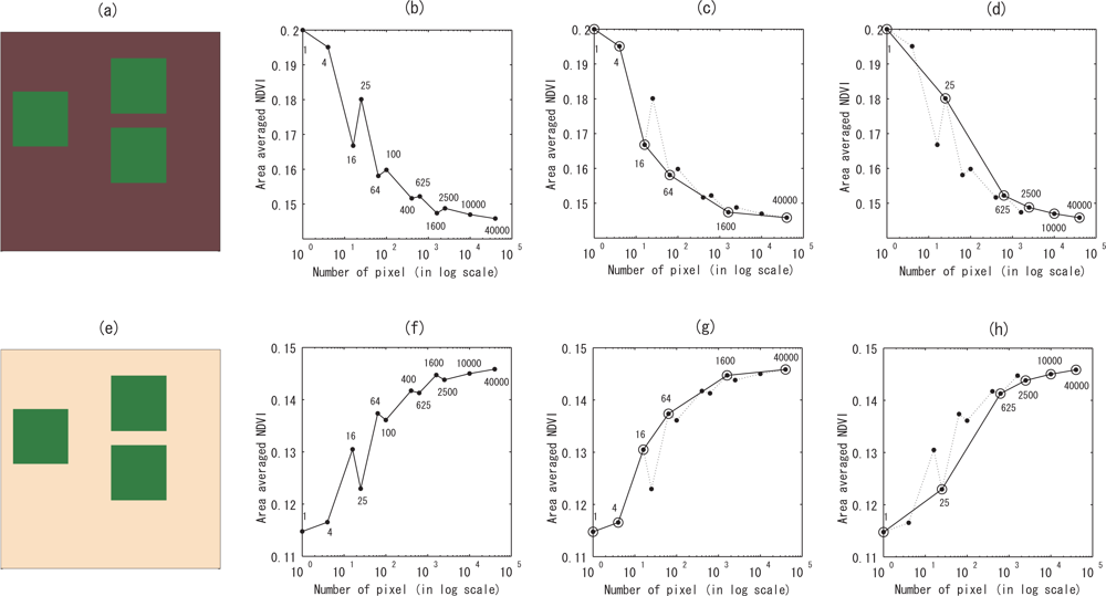
Numerical simulations were conducted to verify the monotonic behavior of the area-averaged NDVI. To this end, we considered two areas of the same size that included both vegetation and non-vegetation endmembers, as shown in Figure 9(a,e). The two areas were identical except that the endmember spectra differed. The endmember spectra in each area were determined to follow decreasing or increasing trends for the average NDVI in Figure 9(a,e), respectively. In other words, η was larger than 1 in Figure 9(a) and smaller than 1 in Figure 9(e).

The target field was assumed to be acquired at the N-th resolution. Note that the pixel size was significantly smaller than any scene object at this resolution. For the simulation, we generated all possible resolutions of the spectral data based on the original data (at the N-th resolution) by arithmetic averaging using a moving block window under the following conditions: (1) the number of rows and columns in the resolution data set remains constant, and (2) each pixel is an element of a square grid. We define a set B that includes elements of all divisors of n (the square root of N), l,

$$B=\left\{l;l\in {\mathit{Z}}_{+},l|n\right\}.$$

(37)

where Z₊ represents the set of positive integers. Then all possible members of the N -th resolution under the limited conditions are represented by a set A_N as

$$A_N=\left\{L;L\in {\mathit{Z}}_{\mathit{+}},L=l^2,l\in B\right\}.$$

(38)

Members of the resolution class are selected from the set A_N in the simulations. To define a general representation of the set of members in a resolution class (C ⊂ A_N), the members of C are indicated as {c₁, c₂, c₃, ···, c_n} under the condition

$$z\sqrt{c_n}=\sqrt{c_{n+1}},$$

(39)

where z ∈ Z₊ and z ≠ 1.

In this simulation, we assumed N was 40000, then A₄₀₀₀₀ becomes

$$A_{40000}=\{1,\hspace{0.17em}4,\hspace{0.17em}16,\hspace{0.17em}25,\hspace{0.17em}64,\hspace{0.17em}100,\hspace{0.17em}400,\hspace{0.17em}625,\hspace{0.17em}1600,\hspace{0.17em}2500,\hspace{0.17em}10000,\hspace{0.17em}40000\}.$$

(40)

The monotonic trend within the resolution class was verified by selecting two examples of the resolution class that satisfied Equation (39), containing five elements. For example, the subsets C₁ ⊂ A₄₀₀₀₀ and C₂ ⊂ A₄₀₀₀₀ were assumed to be

$$C_1=\{1,\hspace{0.17em}4,\hspace{0.17em}16,\hspace{0.17em}64,\hspace{0.17em}1600,\hspace{0.17em}40000\},$$

(41)

$$C_2=\{1,\hspace{0.17em}25,\hspace{0.17em}625,\hspace{0.17em}2500,\hspace{0.17em}10000,40000\}.$$

(42)

The subsets (resolution class) C₁ and C₂ can be referred to as ‘class-1’ and ‘class-2’, respectively, as illustrated in Figure 10. According to the findings discussed in the previous section, the area-averaged NDVI did not vary monotonically over the resolution sequence comprising set A₄₀₀₀₀. On the other hand, the area-averaged NDVI varied monotonically over the resolution class sets (C₁ and C₂).

Figure 9(b,f) shows that the average NDVI varied non-monotonically if the resolution sequence included two classes (class-1 and class-2). The average NDVI certainly behaved monotonically within a single class. The average NDVI within a single class (indicated by the solid line) decreased monotonically, as plotted in Figure 9(c,d) for class-1. The same observation held for the increasing case (class-2) shown in Figure 9(g,h) for class-2.

6. Discussion

A resolution transform model with a certain partitioning rule was proposed to analyze the area-averaged NDVI for a fixed area described under different spatial resolutions. To elucidate the error bounds on the calculated NDVI, the resolution class (condition for monotonicity) was introduced. The resolution class indicates the values that are interconnected under the forward and reverse application of the partitioning rule. Within a class, the area-averaged NDVI certainly vary monotonically with the spatial resolution. The trends in the average NDVI (decreasing or increasing) within a resolution class can be determined based on the factor η calculated for a given NDVI, in agreement with the scaling effects predicted in a numerical study [39]. As a consequence, the values of the VI at extreme resolutions (at the coarsest and finest resolutions) should reach maximum or minimum values because (1) the average NDVI varied monotonically within a resolution class, (2) extreme resolutions belong to the same resolution class, and (3) any resolution certainly belongs to one resolution class. These results indicate that the error bounds on the inherent uncertainties due to the scaling effects can be specified by the maximum and minimum values.

A major limitation of this work is the number of endmember spectra assumed in the LMM. This limitation may cause a loss of practicality in some extent, since in general one encounters more numbers of distinct surfaces within a satellite imagery. This assumption, however, is reasonable at this stage of investigation for the following reason. The monotonicity of NDVI in the framework of scaling issue has not been fully and thoroughly investigated to date. As an initial step of tackling the theme, it is appropriate to start with the simplest case. Moreover, this assumption enables us to analyze the influence of spatial resolution analytically from the beginning to the end. And, owing to this simplicity, one can even reach the understanding of deep insight of the complex phenomena with no ambiguity. Therefore, the assumption brings us both advantage and disadvantage.

The assumption is indeed not practical knowing the fact that pixel size of sensors with middle to lower resolution (with wide field-of-view) is most likely large enough to include three or more numbers of endmember species. Nevertheless, considering the trend of sensor technology, spatial resolution of future sensor will tend to be higher. As a consequence, the pixel size eventually becomes fine enough to the level such that region of interest can be considered as a two-endmember case. In this sense, the results and findings from this study would serve as theory that reasonably explains behavior of scaling effect with some degrees of practicality.

7. Conclusions

We analytically investigated the mechanisms underlying the scaling effects present in the calculation of NDVI under a two-endmember LMM, and we related the scaling effects to the monotonic behavior as a function of the spatial resolution. The scaling effects depended on the spectral features, and this relationship was clarified to show that the trend (increasing or decreasing) depended on the vegetation and non-vegetation endmember spectra. The proof of the monotonicity indicates that the error bounds may be derived deterministically using the area-averaged values calculated from the data at the extreme resolutions.

This study establishes a theoretical framework for describing the scaling effects in the calculation of biophysical or climatological parameters retrieved from remotely sensed data. In this framework, remotely sensed data is modeled using a linear mixture of endmember spectra. The applicability of the results and the findings of this study are mostly restricted by the assumption of two endmembers. Further investigations are required to expand the discussion to (1) the analysis of a greater number of endmembers, and (2) the analysis of other biophysical parameters, such as LAI or FAPAR. Nevertheless, the fundamental behavior of the scaling effects form a theoretical basis for similar investigations.

References

- Myneni, R.B.; Keeling, C.D.; Tucker, C.J.; Asrar, G.; Nemani, R.R. Increased plant growth in the northern high latitudes from 1981 to 1991. Nature 1997, 386, 698–702. [Google Scholar]
- Los, S.O.; Pollack, N.H.; Parris, M.T.; Collatz, G.J.; Tucker, C.J.; Sellers, P.J.; Malmstrom, C.M.; DeFries, R.S.; Bounoua, L.; Dazlich, D.A. A global 9-yr biophysical land surface dataset from NOAA AVHRR data. J. Hydrometeorol 2000, 1, 183–199. [Google Scholar]
- Sellers, P.J.; Los, S.O.; Tucker, C.J.; Justice, C.O.; Dazlich, D.A.; Collatz, G.J.; Randall, D.A. A revised land surface parameterization (SiB2) for atmospheric GCMS. Part I: Model formulation. J. Climate 1996, 9, 676–705. [Google Scholar]
- Sellers, P.J.; Randall, D.A.; Collatz, G.J.; Berry, J.A.; Field, C.B.; Dazlich, D.A.; Zhang, C.; Collelo, G.D.; Bounoua, L. A revised land surface parameterization(SiB2) for atmospheric GCMs. Part II: the generation of global fields of terrestrial biophysical parameters from satellite data. J. Climate 1996, 9, 706–737. [Google Scholar]
- Jarlan, L.; Mangiarotti, S.; Mougin, E.; Mazzega, P.; Hiernaux, P.; Dantec, V.L. Assimilation of SPOT/VEGETATION NDVI data into a sahelian vegetation dynamics model. Remote Sens. Environ 2008, 112, 1381–1394. [Google Scholar]
- Goetz, S.J. Multi-sensor analysis of NDVI, surface temperature and biophysical variables at a mixed grassland site. Int. J. Remote Sens 1997, 18, 71–94. [Google Scholar]
- Pottier, C.; Garcon, V.; Larnicol, G.; Sudre, G.; Schaeffer, P.; Traon, P.Y.L. Merging SeaWIFS and MODIS/Aqua ocean color data in North and Equatorial Atlantic using weighted averaging and objective analysis. IEEE Trans. Geosci. Remote Sens 2006, 44, 3436–3451. [Google Scholar]
- Tucker, C.J.; Pinzon, J.E.; Brown, M.E.; Slayback, D.A.; Pak, E.W.; Mahoney, R.; Vermote, E.F.; Saleous, N.E. An extended AVHRR 8-km NDVI dataset compatible with MODIS and SPOT vegetation NDVI data. Int. J. Remote Sens 2005, 26, 4485–4498. [Google Scholar]
- Pohl, C.; Van Genderen, J.L. Multisensor image fusion in remote sensing: Concepts, methods and applications. Int. J. Remote Sens 1998, 19, 823–854. [Google Scholar]
- Price, J.C. Combining multispectral data of differing spatial resolution. IEEE Trans. Geosci. Remote Sens 1999, 37, 1199–1203. [Google Scholar]
- Brown, M.; Pinzon, J.; Didan, K.; Morisette, J.; Tucker, C. Evaluation of the consistency of long-term NDVI time series derived from AVHRR,SPOT-vegetation, SeaWiFS, MODIS, and Landsat ETM+ sensors. IEEE Trans. Geosci. Remote Sens 2006, 44, 1787–1793. [Google Scholar]
- Wulder, M.A.; Butson, C.R.; White, J.C. Cross-sensor change detection over a forested landscape: Options to enable continuity of medium spatial resolution measures. Remote Sens. Environ 2008, 112, 796–809. [Google Scholar]
- Pouliot, D.; Latifovic, R.; Fernandes, R.; Olthof, I. Evaluation of compositing period and AVHRR and MERIS combination for improvement of spring phenology detection in deciduous forests. Remote Sens. Environ 2011, 115, 158–166. [Google Scholar]
- Arai, E.; Shimabukuro, Y.E.; Pereira, G.; Vijaykumar, N.L. A multi-resolution multi-temporal technique for detecting and mapping deforestation in the Brazilian Amazon rainforest. Remote Sens 2011, 3, 1943–1956. [Google Scholar]
- Stellmes, M.; Udelhoven, T.; Roder, A.; Sonnenschein, R.; Hill, J. Dryland observation at local and regional scale—Comparison of Landsat TM/ETM+ and NOAA AVHRR time series. Remote Sens. Environ 2010, 114, 2111–2125. [Google Scholar]
- Townshend, J.R.G.; Justice, C.O. Selecting the spatial resolution of satellite sensors required for global monitoring of land transformations. Int. J. Remote Sens 1988, 9, 187–236. [Google Scholar]
- van Leeuwen, W.J.; Orr, B.J.; Marsh, S.E.; Herrmann, S.M. Multi-sensor NDVI data continuity: Uncertainties and implications for vegetation monitoring applications. Remote Sens. Environ 2006, 100, 67–81. [Google Scholar]
- Ganguly, S.; Schull, M.A.; Samanta, A.; Shabanov, N.V.; Milesi, C.; Nemani, R.R.; Knyazikhin, Y.; Myneni, R.B. Generating vegetation leaf area index earth system data record from multiple sensors. Part 1: Theory. Remote Sens. Environ 2008, 112, 4333–4343. [Google Scholar]
- Zhao, T.; Bergen, K.M.; Brown, D.G.; Shugart, H.H. Scale dependence in quantification of land-cover and biomass change over Siberian boreal forest landscapes. Landscape Ecol 2009, 24, 1299–1313. [Google Scholar]
- Miura, T.; Huete, A.; Yoshioka, H. An empirical investigation of cross-sensor relationships of NDVI and red/near-infrared reflectance using EO-1 Hyperion data. Remote Sens. Environ 2006, 100, 223–236. [Google Scholar]
- Bounoua, L.; Collatz, G.J.; Los, S.O.; Sellers, P.J.; Dazlich, D.A.; Tucker, C.J.; Randall, D.A. Sensitivity of climate to changes in NDVI. J. Climate 2000, 13, 2277–2292. [Google Scholar]
- McConnell, M.; Weidman, S. Uncertainty Management in Remote Sensing of Climate Data: Summary of a Workshop; The National Academies Press: Washington, DC, USA, 2009. [Google Scholar]
- Overpeck, J.T.; Meehl, G.A.; Bony, S.; Easterling, D.R. Climate data challenges in the 21st Century. Science 2011, 331, 700–702. [Google Scholar]
- Hu, Z.; Islam, S. A frame work for analyzing and designing scale invariant remote sensing algorithms. IEEE Trans. Geosci. Remote Sens 1997, 35, 747–755. [Google Scholar]
- Jiang, Z.; Huete, A.R.; Chen, J.; Chen, Y.; Yan, G.; Zhang, X. Analysis of NDVI and scaled difference vegetation index retrievals of vegetation fraction. Remote Sens. Environ 2006, 101, 366–378. [Google Scholar]
- Wu, H.; Li, Z.L. Scale issues in remote sensing: A review on analysis, processing and modeling. Sensors 2009, 9, 1768–1793. [Google Scholar]
- Chen, J.M. Spatial scaling of a remotely sensed surface parameter by contexture. Remote Sens. Environ 1999, 69, 30–42. [Google Scholar]
- Settle, J. On the use of remotely sensed data to extimate spatially averaged geophysical variables. IEEE Trans. Geosci. Remote Sens 2004, 42, 620–631. [Google Scholar]
- Settle, J.J. On the residual term in the linear mixture model and its dependence on the point spread function. IEEE Trans. Geosci. Remote Sens 2005, 43, 398–401. [Google Scholar]
- Hall, F.G.; Huemmrich, K.F.; Goetz, S.J.; Sellers, P.J.; Nickeson, J.E. Satellite remote sensing of surface energy balance: Success, failures, and unresolved issues in FIFE. J. Geophys. Res 1992, 97, 19061–19089. [Google Scholar]
- Friedl, M.A.; Davis, F.W.; Michaelsen, J.; Moritz, M.A. Scaling and uncertainty in the relationship between the NDVI and land surface biophysical variables: An analysis using a scene simulation model and data from FIFE. Remote Sens. Environ 1995, 54, 233–246. [Google Scholar]
- Sprintsin, M.; Karnieli, A.; Berliner, P.; Rotenberg, E.; Yakir, D.; Cohen, S. The effect of spatial resolution on the accuracy of leaf area index estimation for a forest planted in the desert transition zone. Remote Sens. Environ 2007, 109, 416–428. [Google Scholar]
- Zhang, X.; Yan, G.; Li, Q.; Li, Z.L.; Wan, H.; Guo, Z. Evaluating the fraction of vegetation cover based on NDVI spatial scale correction model. Int. J. Remote Sens 2006, 27, 5359–5372. [Google Scholar]
- Garrigues, S.; Allard, D.; Baret, F.; Weiss, M. Quantifying spatial heterogeneity at the landscape scale using variogram models. Remote Sens. Environ 2006, 103, 81–96. [Google Scholar]
- Ma, L.; Li, C.; Tang, B.; Tang, L.; Bi, Y.; Zhou, B.; Li, Z.L. Impact of spatial LAI heterogeneity on estimate of directional gap fraction from SPOT-satellite data. Sensors 2008, 8, 3767–3779. [Google Scholar]
- Zheng, G.; Moskal, L.M. Retrieving Leaf Area Index(LAI) using remote sensing: Theories, method and sensors. Sensors 2009, 9, 2719–2745. [Google Scholar]
- Tao, X.; Yan, B.; Wang, K.; Wu, D.; Fan, W.; Xu, X.; Liang, S. Scale transformation of Leaf Area Index product retrieved from multiresolution remotely sensed data: Analysis and case studies. Int. J. Remote Sens 2009, 30, 5383–5395. [Google Scholar]
- Aman, A.; Randriamanantena, H.P.; Podaire, A.; Frouin, R. Upscale integration of normalized difference vegetation index: the problem of spatial heterogeneity. IEEE Trans. Geosci. Remote Sens 1992, 30, 326–338. [Google Scholar]
- Huete, A.; Kim, H.J.; Miura, T. Scaling Dependencies and Uncertainties in Vegetation Index—Biophysical Retrievals in Heterogeneous Environments. Proceedings of 2005 IEEE International Geoscience and Remote Sensing Symposium, Seoul, Korea, 25–29 July 2005; 7, pp. 5029–5032.
- Thenkabail, P.S. Inter-sensor relationships between IKONOS and Landsat-7 ETM+ NDVI data in three ecoregions of Africa. Int. J. Remote Sens 2004, 20, 389–408. [Google Scholar]
- Maselli, F.; Gilabert, M.A.; Conse, C. Integration of high and low resolution NDVI data for monitoring vegetation in Mediterranean environments. Remote Sens. Environ 1998, 63, 208–218. [Google Scholar]
- Wood, E.F.; Lakshmi, V. Scaling water and energy fluxes in climate systems: Three land-atmospheric modeling experiments. J. Climate 1993, 6, 839–857. [Google Scholar]
- Price, J.C. Using spatial context in satellite data to infer regional scale evapotranspiration. IEEE Trans. Geosci. Remote Sens 1990, 28, 940–948. [Google Scholar]
- Cola, L.D. Multiresolution covariation among Landsat and AVHRR vegetation indices. In Scale in Remote Sensing and GIS; Quattrochi, D.A., Goodchild, M.F., Eds.; Lewis: Boca Raton, FL, USA, 1997; pp. 73–91. [Google Scholar]
- Liang, S. Numerical experiments on the spatial scaling of land surface albedo and leaf area index. Int. J. Remote Sens 2000, 19, 225–242. [Google Scholar]
- Garrigues, S.; Allard, D.; Baret, F.; Weiss, M. Influence of landscape spatial heterogeneity on the non-linear estimation of leaf area index from moderate spatial resolution remote sensing data. Remote Sens. Environ 2006, 105, 286–298. [Google Scholar]
- Hu, Z.; Islam, S. Effects of subgrid-scale heterogeneity of soil wetness and temperature on grid-scale evaporation and its parameterization. Int. J. Climatol 1998, 18, 49–63. [Google Scholar]
- Bonan, G.B.; Pollard, D.; Thompson, S.L. Influence of subgrid-scale heterogeneity in leaf area index, stomatal resistance, and soil moisture on grid-scale land-atmosphere interactions. J. Climate 1993, 6, 1883–1897. [Google Scholar]
- Pielke, R.A.; Dalu, G.A.; Snook, J.S.; Lee, T.J.; Kittel, T.G. Nonlinear influence of mesoscale land use on weather and climate. J. Climate 1991, 4, 1053–1069. [Google Scholar]
- Marht, L.; Sun, J. Dependence of surface exchange coefficients on averaging scale and grid size. Q. J. Roy. Meteorol. Soc 1995, 121, 1835–1852. [Google Scholar]
- Maayar, M.E.; Chen, J.M. Spatial scaling of evapotranspiration as affected by heterogeneities in vegetation, topography, and soil texture. Remote Sens. Environ 2006, 102, 33–51. [Google Scholar]
- Chen, B.; Chen, J.M.; Mo, G.; Yuen, C.W.; Margolis, H.; Higuchi, K.; Chan, D. Modeling and scaling coupled energy, water, and carbon fluxes based on remote sensing: An application to Canada’s landmass. J. Hydrometeorol 2007, 8, 123–143. [Google Scholar]
- Simic, A.; Chen, J.M.; Liu, J.; Csillag, F. Spatial scaling of net primary productivity using subpixel information. Remote Sens. Environ 2004, 93, 246–258. [Google Scholar]
- Zheng, D.; Heath, L.S.; Ducey, M.J.; Smith, J.E. Quantifying scaling effects on satellite-derived forest area estimates for the conterminous USA. Int. J. Remote Sens 2009, 30, 3097–3114. [Google Scholar]
- Propastin, P.A. Spatial non-stationarity and scale-dependency of prediction accuracy in the remote estimation of LAI over a tropical rainforest in Sulawesi, Indonesia. Remote Sens. Environ 2009, 113, 2234–2242. [Google Scholar]
- Raffy, M. Change of scale in models of remote sensing: A general method for spatialization of models. Remote Sens. Environ 1992, 40, 101–112. [Google Scholar]
- Raffy, M. Heterogeneity and change of scale in models of remote sensing. Int. J. Remote Sens 1994, 15, 2359–2380. [Google Scholar]
- Yoshioka, H.; Wada, T.; Obata, K.; Miura, T. Monotonicity of Area Averaged NDVI as a Function of Spatial Resolution Based on a Variable Endmember Linear Mixture Model. Proceedings of 2008 IEEE International Geoscience & Remote Sensing Symposium, Boston, MA, USA, 6–11 July 2008; III, pp. 415–418.
- Horwitz, H.M.; Nalepka, R.F.; Hyde, P.D.; Morgenstern, J.P. Estimating the Proportions of Objects within a Single Resolution Element of a Multispectral Scanner. Proceedings of 7th International Symposium on Remote Sensing of Environment, Ann Arbor, MI, USA, 17–21 may 1971; pp. 1307–1320.
- Smith, M.O.; Johnson, P.E.; Adams, J.B. Quantitative determination of mineral types and abundances from reflectance spectra using principal components analysis. J. Geophys. Res 1985, 90 Suppl., C797–C804. [Google Scholar]
- Adams, J.B.; Smith, M.O.; Johnson, P.E. Spectral mixture modeling: A new analysis of rock and soil types at the Viking Lander 1 Site. J. Geophys. Res 1986, 91, 8098–8112. [Google Scholar]
- Smith, M.O.; Ustin, S.L.; Adams, J.B.; Gillespie, A.R. Vegetation in deserts: I. A regional measure of abundance from multispectral images. Remote Sens. Environ 1990, 31, 1–26. [Google Scholar]
- Settle, J.J.; Drake, N.A. Linear mixing and the estimation of ground cover proportions. Int. J. Remote Sens 1993, 14, 1159–1177. [Google Scholar]
Figure 1.
Non-monotonic behavior on an area-averaged NDVI as a function of the number of pixels (spatial resolution) over a fixed area. (a), (b), or (c) illustrate the hypothetical image obtained for one, four, or nine pixels within a fixed area that includes vegetation and soil backgrounds. The vegetation spectrum (covering both red and NIR reflectance spectra) is assumed to be (0.05, 0.4), and the soil background spectrum is (0.15, 0.15). (d) The area-averaged NDVI as a function of the number of pixels.
Figure 2.
Elements of the resolution transformation process based on a simple partitioning procedure.
Figure 3.
Illustration of the resolution transform using the partitioning rule. The upper panel shows an example of the resolution transform from levels 1 to 4, and the lower panel shows the transform from levels 1 to 9.
Figure 4.
The endmember abundances of the vegetated surface (fraction of vegetation cover) for pixel k under the j-th resolution is represented by ωj,k.
Figure 5.
Illustration of the variables used in this study. v̄j indicates the area-averaged NDVI at the j-th resolution. vj,k indicates the NDVI calculated for pixel k under the j-th resolution. ρj,k is the reflectance spectrum of pixel k at a resolution of j and is a linear combination of the vegetation and non-vegetation endmember spectra, ρv and ρs with weights ωj,k.
Figure 6.
The fraction of a pixel after the partitioning process, represented by α.
Figure 7.
Monotonicity of the area-averaged NDVI in consecutive resolution sequences. A trend increases or decreases depending on the factor η.
Figure 8.
Illustration of the resolution transform from resolution levels 1 to 4. (a) and (b) describe the elements of the resolution sequences class A and class B, respectively. (c) depicts the elements of a resolution sequence in which elements from both class A and class B are included. The average NDVI varies monotonically in (a) and (b). In contrast, non-monotonic behavior is observed in (c) at the resolution level 3.
Figure 9.
Numerical demonstration of the scaling effects in the calculation of the area-averaged NDVI. (a) Hypothetical field over which was observed a vegetation endmember spectrum of (ρr, ρn) = (0.05, 0.4) and a non-vegetation endmember spectrum of (0.15,0.15). (b–d) present the average NDVI calculated from the field (a). (b) Variations in the average NDVI, including the two resolution classes (set A40000); (c) Variations within class-1 (subset C1) only, or (d) for class-2 (subset C2) only. (e) A hypothetical field over which was observed a vegetation endmember spectrum of (0.05,0.4) and a non-vegetation endmember spectrum of (0.3,0.3). (f–h) present the average NDVI calculated from the field (e). (f) Variations in the average NDVI over the two resolution classes; (g) Variations within class-1 only, or (h) for class-2 only.
Figure 10.
Two resolution classes used in the experiments. The upper sequence (class-1, C1) presents a different class than the lower sequence (class-2, C2).
Share and Cite
MDPI and ACS Style
Obata, K.; Wada, T.; Miura, T.; Yoshioka, H. Scaling Effect of Area-Averaged NDVI: Monotonicity along the Spatial Resolution. Remote Sens. 2012, 4, 160-179. https://0-doi-org.brum.beds.ac.uk/10.3390/rs4010160
AMA Style
Obata K, Wada T, Miura T, Yoshioka H. Scaling Effect of Area-Averaged NDVI: Monotonicity along the Spatial Resolution. Remote Sensing. 2012; 4(1):160-179. https://0-doi-org.brum.beds.ac.uk/10.3390/rs4010160
Chicago/Turabian StyleObata, Kenta, Takahiro Wada, Tomoaki Miura, and Hiroki Yoshioka. 2012. "Scaling Effect of Area-Averaged NDVI: Monotonicity along the Spatial Resolution" Remote Sensing 4, no. 1: 160-179. https://0-doi-org.brum.beds.ac.uk/10.3390/rs4010160