Use of Variogram Parameters in Analysis of Hyperspectral Imaging Data Acquired from Dual-Stressed Crop Leaves

1
Texas AgriLife Research, Texas A&M System, 1102 East FM 1294, Lubbock, TX 79403, USA
2
The UWA Institute of Agriculture, School of Animal Biology, The University of Western Australia, 35 Stirling Highway, Crawley, Perth, WA 6009, Australia
Remote Sens. 2012, 4(1), 180-193; https://0-doi-org.brum.beds.ac.uk/10.3390/rs4010180
Submission received: 25 October 2011
/
Revised: 10 January 2012
/
Accepted: 10 January 2012
/
Published: 11 January 2012
(This article belongs to the Special Issue Hyperspectral Remote Sensing)
Abstract
:A detailed introduction to variogram analysis of reflectance data is provided, and variogram parameters (nugget, sill, and range values) were examined as possible indicators of abiotic (irrigation regime) and biotic (spider mite infestation) stressors. Reflectance data was acquired from 2 maize hybrids (Zea mays L.) at multiple time points in 2 data sets (229 hyperspectral images), and data from 160 individual spectral bands in the spectrum from 405 to 907 nm were analyzed. Based on 480 analyses of variance (160 spectral bands × 3 variogram parameters), it was seen that most of the combinations of spectral bands and variogram parameters were unsuitable as stress indicators mainly because of significant difference between the 2 data sets. However, several combinations of spectral bands and variogram parameters (especially nugget values) could be considered unique indicators of either abiotic or biotic stress. Furthermore, nugget values at 683 and 775 nm responded significantly to abiotic stress, and nugget values at 731 nm and range values at 715 nm responded significantly to biotic stress. Based on qualitative characterization of actual hyperspectral images, it was seen that even subtle changes in spatial patterns of reflectance values can elicit several-fold changes in variogram parameters despite non-significant changes in average and median reflectance values and in width of 95% confidence limits. Such scattered stress expression is in accordance with documented within-leaf variation in both mineral content and chlorophyll concentration and therefore supports the need for reflectance-based stress detection at a high spatial resolution (many hyperspectral reflectance profiles acquired from a single leaf) and may be used to explain or characterize within-leaf foraging patterns of herbivorous arthropods.
1. Introduction
There are numerous studies of stress detection in crop leaves based on reflectance data acquired with either single sensor devices or imaging devices, including: biotic stress [1–4], salinity stress [5], nutrient deficiency [6], and drought stress [3,7]. Carter and Knapp [8] provided a thorough review of reflectance based detection of abiotic and biotic stressors (including dehydration, flooding, freezing, ozone, herbicides, competition, disease, insects, and deficiencies in ectomycorrhizal development and N fertilization) within the 400–850 nm wavelength range when imposed on a wide range of plant species (grasses, conifers, and deciduous trees). Irrespectively of abiotic or abiotic stressor, Carter and Knapp [8] concluded that in most studies there appears to be an increase in reflectance in response to plant stress, and this increase is generally most noticeable near the red edge at 700 nm. A possible explanation for such increase in reflectance is that stressors partially compromise the photosynthetic efficiency of the plant, so comparatively more radiometric energy is reflected back to the atmosphere than from a non-stressed plant. If such increase in leaf reflectance occurs in response to a given stressor, then a follow-up question is whether it is due to a general reflectance increase across a given leaf (in all pixels) or whether it is associated with proportionally higher reflectance in scattered points within each leaf? Several studies have demonstrated within-leaf variation in distribution of minerals [9] and chlorophyll [10], so it seems reasonable to assume that there is spatial variability within a leaf in terms of expression of stress response. In addition to important questions about the spatial distribution of stress expression within leaves, it is also important to address a spectral aspect of the findings by Carter and Knapp [8]. From an academic standpoint, it is obviously quite interesting that plants tend to have a quase-universal stress reflectance response near 700 nm, but it means that practical applications of reflectance based stress detection systems may be limited, unless more unique reflectance features can be associated with different abiotic and biotic stressors. That is, under real-world/commercial conditions crop plants will likely be adversely affected by several stressors simultaneously, and/or there may be important interactions between stressors. Thus, specific stress detection tools are needed, so that different stressors can be detected and quantified independently. For instance, it is widely known that crops become more susceptible to spider mite (Acari: Tetranychidae) infestations (example of biotic stressor), when crops are grown under drought stressed conditions (cotton, Gossypium spp. [11], sorghum, Sorghum bicolor (L.) Moench [12], and maize [13–15]). This association between spider mites and drought stress suggests that early detection of drought stress can possibly serve 2 complementary purposes: (1) to optimize irrigation regimes, and (2) alert growers about when pro-active miticide applications may be warranted. It is important to emphasize that reflectance based detection of crop stress is mainly of interest if it can be used to detect emerging adverse effects of abiotic and/or biotoc stressors, before symptoms become obvious to the Human eye. In other words, the true potential of reflectance based detection is associated with an ability to detect subtle/emerging stress levels, so that management practices can be adjusted before significant crop yield losses have occurred. In addition, several studies have described reflectance based detection of emerging spider mite infestations [1,3,4].
Recently, use of variogram parameters has been demonstrated as well-suited for dual-detection of abiotic and biotic stress in crop plants [3,4,16]. However, better insight into the relationship between reflectance values and variogram parameters is needed in order to interpret and discuss variogram parameters as stress indicators in an agro-ecological context and to understand within-leaf stress expression. The main purpose of this study was 3-fold: (1) provide a detailed theoretical description of variogram analysis when applied to reflectance data from hyperspectral images, (2) identify combinations of spectral ranges between 405 and 907 nm and variogram parameters, which may be considered suitable for detection of abiotic (experimental irrigation regimes) and biotic [spider mites (Acari: Tetranychidae)] stressors, and (3) based on descriptive statistics and visualization of imaging data, characterize spectral responses to abiotic and biotic stressors. Thus, this study provides detailed insight into the relationships between stressors’ effect on reflectance values within crop leaves and between reflectance values and estimated variogram parameters. Due to the interest in detection and characterization of subtle/emerging stress levels, maize plants were subjected to fairly modest levels of abiotic and biotic stress levels.
2. Variogram Analysis: A Theoretical Background
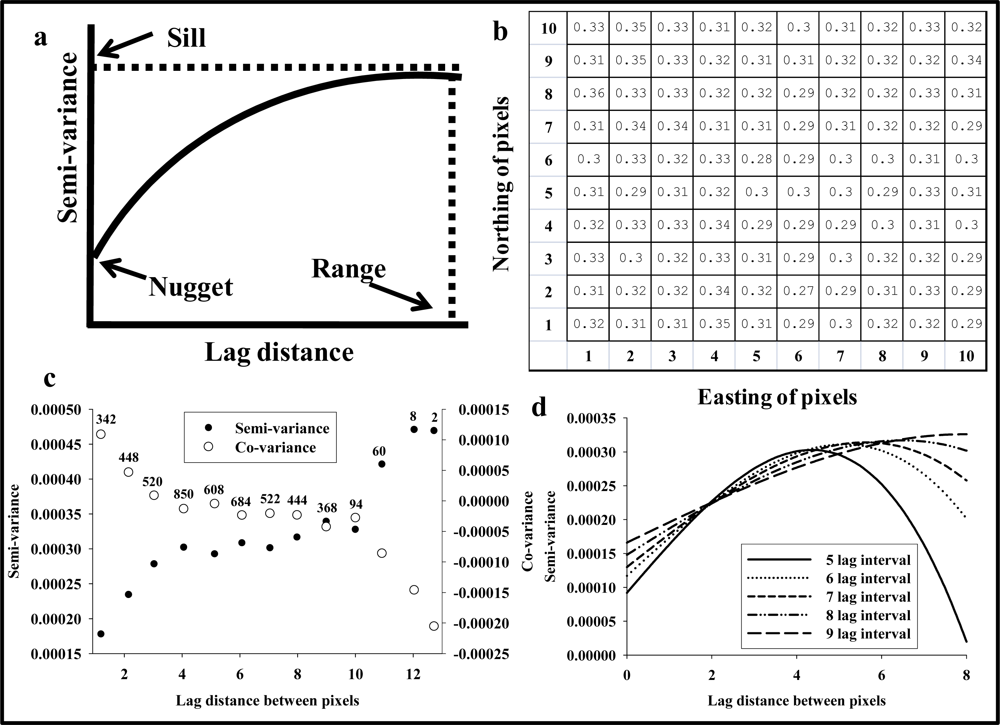
In the 1930’s, geostatistics were conceptually proposed by Dr. Krige as an approach to optimize gold ore mining in Southern Africa, and Dr. Matheron developed the mathematical models of this concept in the 1960’s and 1970’s [17]. Today with geographic information systems (GIS) being applied to epidemiological, ecological, socio-economic, oceanographic, meteorological and many other types of studies, geostatistics as a discipline is widely accepted as being 1 of the most powerful and robust approaches to spatial data analysis. For more exhaustive descriptions of variogram analysis, it is recommended to consult Armstrong [17] and Isaaks and Srivastava [18]. The fundamental assumption of geostatistics is that difference (i.e., semi-variance or co-variance) in reflectance values between points within the image cube is correlated with the distance between pixels. Furthermore, it is assumed possible to develop a model that describes the spatial structure or relationship between distance between pixels and variance of reflectance values. This type of spatial structure analysis can be conducted with reflectance data from hyperspectral images, because each pixel (hyperspectral profile) is in a grid with a set of x- and y-coordinates within each image cube. Importantly, traditional applications of geostatistics involve data sets where only a restricted number of point observations are known (i.e., drilling holes in an area with high likelihood of gold deposits), and most commonly 1 of the principal objectives associated with geostatistical analyses is directly linked to predictions of counts at unsampled locations (i.e., to predict the highest likelihood of rich gold deposits). Regarding hyperspectral images, the entire “data universe” is known, that is, actual reflectance values are available from all geographic positions (pixels), so the objective is not to predict values at unsampled locations but to characterize their spatial structure and use the spatial structure as an indicator of the target object, in this case stress expression within maize leaves. In other words, it is assumed that reflectance data acquired from different target objects (for instance, crop leaves from plants subjected to different stress levels) also will have different spatial structures. A semi-variogram analysis characterizes the relationship between distance between paired observations and the semi-variance (variance divided by 2) of observations of these paired observations (Figure 1(a)). The spatial structure of a given data set is either random or non-random. Random, or lack of spatial dependence, means that the variance associated with reflectance values within an image is independent of the distance between pixels. The curve fit in the semi-variogram is a straight line denoted “pure nugget variogram” [19]. A data set with non-random spatial structure, shows spatial dependence [19,20] or spatial continuity [18]. Non-random, spatial dependence among observations points may follow an asymptotic curve that gradually increases with lag distance up to a certain point by which the variance of counts levels off and becomes random, which is the distance by which point observations (i.e., reflectance values in a single spectral band) are no longer spatially correlated (Figure 1(a)). As part of developing the variogram, a regression curve fit is used to model the spatial structure and estimate 3 standard parameters: “nugget”, “range”, and “sill” (Figure 1(a)). The nugget represents an estimate of the semi-variance or co-variance between observations collected at “zero lag distance apart” or 2 reflectance values from the same pixel. Theoretically the nugget should be zero for semi-variance and infinitely high for co-variance, and it equals the noise or stochasticity in the data set. The sill is an estimate of the total variance explained by the spatial structure analysis. The range is an estimate of the maximum distance at which point observations are spatially correlated, beyond this lag distance interval point observations are to be considered spatially uncorrelated. Two regression fits are commonly used in regression fits of variogram data:
is an exponential curve fit [18], in which “a” denotes the nugget, “b” the sill, and “c” the “range”.
is an spherical curve fit [18], in which “a” denotes the nugget, “b” the sill, and “c” the “range”.
The procedures of spatial structure analysis applied to hyperspectral imaging data are best explained with an example, in this case reflectance values from a maize leaf in a single spectral band and with 100 pixels arranged in a 10 by 10 grid pattern (Figure 1(b)). Accordingly, the distance between paired pixels ranges from 1 to 14.1, and the total number of paired distances (N) is 4,950 (Equation (3)).
The 4,950 distance combinations are grouped into fixed lag distance intervals, which are projected along the x-axis in a variogram, and the y-axis in a variogram depicts either the average semi-variance or co-variance for each lag distance interval. Obviously, there are not equal numbers of distance pairs for all lag distance intervals, and Figure 1(c) shows semi-variance or co-variance of the data in Figure 1(b) when divided into 13 lag distance intervals. It is seen that there are only 2 distance pairs for the longest lag distance interval, while there were 850 pairs for lag distance = 4. Average semi-variance and co-variance estimates for the first 9 lag distance intervals were based on 340–850 pairs, while estimates for the last 4 lag distance intervals were based on <100 pairs and therefore more erratic. Thus, it can be argued that these lag distance intervals should be excluded as they are based on comparatively less data than the initial 9 estimates of either semi-variance or co-variance. Figure 1(c) also shows that average semi-variance increases and reaches a plateau at a lag distance of about 4, and that is also the lag distance at which the co-variance becomes negative. Plateau of semi-variance and/or negative co-variance suggests a lag distance by which point observations are no longer spatially correlated and that the range value has been reached. Importantly, the range estimate should not exceed the shortest distance within the image file. Thus, regarding the data set presented in Figure 1(c), variogram parameter estimates should be discarded if the range value estimate exceeds 10.
A very important aspect of regression fits to variogram data is the decision on how many lag distance intervals to use when fitting Equations (1) or (2) to the data in Figure 1(b). All regression fits with Equation (2) to semi-variance data when 5–9 lag distance intervals were included (excluding the last 4) provided highly significant regression fits (P < 0.001), but it was seen that range estimates increased with number of lag distance intervals included in the regression fit (Figure 1(d)). In fact, the range estimate with nine lag distance intervals (7.9) was almost twice the range estimate with five lag distance intervals (4.3), and the nugget value was 1.8 times higher when based on 9 lag distance intervals compared to 5. This simple example illustrates how fairly subjective decisions about regression fit settings can markedly affect the outcome of a given variogram analysis. Thus, despite the widespread acceptance of geostatistics being “BLUE” (best linear unbiased estimate) [18,22], it is also sometimes acknowledged that different applicators of this approach may develop highly different spatial structure analyses of the same data set, and a significant portion of this “subjectivity” is associated with decisions made regarding variogram analyses [18,21]. However, a recent analysis of a wide range of variogram settings demonstrated that this analytical approach had higher robustness (radiometric repeatability) than 3 standard vegetation indices (NDVI, SI, and PRI) [16].
3. Materials and Methods
3.1. Greenhouse Plant Material
The greenhouse maize plants have been described elsewhere [3,16]. In brief, we planted 2 maize hybrids (Hybrid 1: Triumph 1416, 2004 and Hybrid 2: Pioneer 3223, 2006) October 2007 (data set 1) and February 2008 (data set 2) in individual 11L plastic pots, and each plant was maintained under 1 of 3 water regimes. Spider mite infestation consisted of placing a heavily infested leaf piece on each maize plant. Maize plants in data set 1 were infested 4 December 2007, while maize plants in data set 2 were infested 25 March 2008.
3.2. Hyperspectral Imaging
A push broom line-scanning hyperspectral camera with 640 sensors in a linear array (PIKA II, www.resonon.com) was used. This hyperspectral camera acquires reflectance data in 160 spectral bands in wavelengths from 405 to 907 nm. Dark calibration was conducted at the beginning of the data acquisition. White Teflon was used for white calibration immediately before each image acquisition to account for subtle changes in light conditions. Each hyperspectral image was 6 cm long and 2.5 cm wide (15 cm2) from mid portion of 7th or 8th leaf without damaging the maize plant (leaf not excised). A hyperspectral image consisted of 160,000 reflectance profiles (640 sensors × 250 frames) or pixels. The imaging device was mounted about 45 cm from imaged leaves and the reflectance data were acquired at a spatial resolution of 106 hyperspectral profiles or pixels per mm2 inside a greenhouse with sunlight as the only light source. Similar to [16], PC-ENVI 4.7 ( www.ittvis.com) was used to conduct 4 × 4 spatial averaging so that each hyperspectral image from greenhouse plants was reduced to 10,080 (160 × 63) pixels. Thus, after spatial averaging of hyperspectral imaging data from greenhouse plants, the spatial resolution was equivalent to 6.7 hyperspectral profiles (pixels) per mm2.
3.3. Variogram Settings
All hyperspectral image files were imported into PC-SAS 9.2 (Cary, NC, USA) for data processing and statistical analyses. Variogram analyses (PROC VARIOGRAM) were conducted of all combinations of spectral bands (160) and hyperspectral images (229) (total = 36,640 variogram analyses). Based on a previous study [4], the following variogram settings were used: semi-variance data with a lag distance of 2 and 15 lag distance intervals. Non-linear regression (Proc nlin) was used to conduct spherical regression (Equation (2)) of semi-variance data and to estimate the 3 variogram parameters, nugget, sill, and range. Variogram parameter estimates from a hyperspectral image file were discarded if the regression fits failed to converge or the predicted range value exceeded 63. This threshold of 63 was chosen as it represented the width of the imaging data cube and a range value higher than 63 meant that the sill was reached at a lag distance that was longer than the width of data set. Due to the range value threshold, there was a slight variation in the number of variogram data observations used in statistical analyses of each of the spectral bands. Each of the 3 variogram parameters, nugget, sill, and range, were examined individually in an analysis of variance (PROC MIXED) with 4 treatment effects (data set, hybrid, abiotic, and biotic stressors) and day after infestation as random variable. Abiotic stress was assigned a value from 1 to 3 with: no drought stress (abiotic stress = 1), moderate (abiotic stress = 2), or high (abiotic stress = 3). These water regimes were imposed by watering highly drought stressed plants one-third as much as the no drought stressed plants, and moderately drought stressed plants received two-thirds of the water given to no drought stressed plants. Spider mite infestations were grouped into the following 3 classes: (1) biotic stress = 1 (0–10 spider mites per plant) (50% of data), (2) biotic stress = 2 (10–480 spider mites per plant) (25% of data), and (3) biotic stress = 3 (>480 spider mites per plant) (25% of data). These ranges were chosen to obtain similar numbers of observations in the 2 classes with spider mite induced stress. For each analysis of a variogram parameter, F-values associated with each of the treatment factors were used as indicators of how well a given combination of spectral band and variogram parameter responded to the examined stress factors.
4. Results and Discussion
4.1. Dual Stress Detection
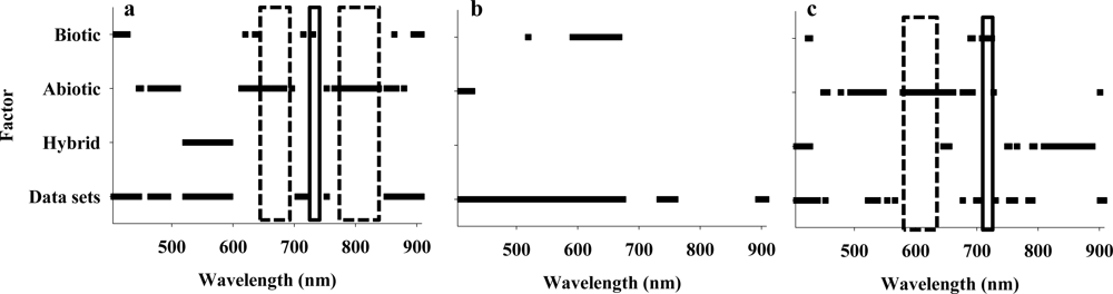
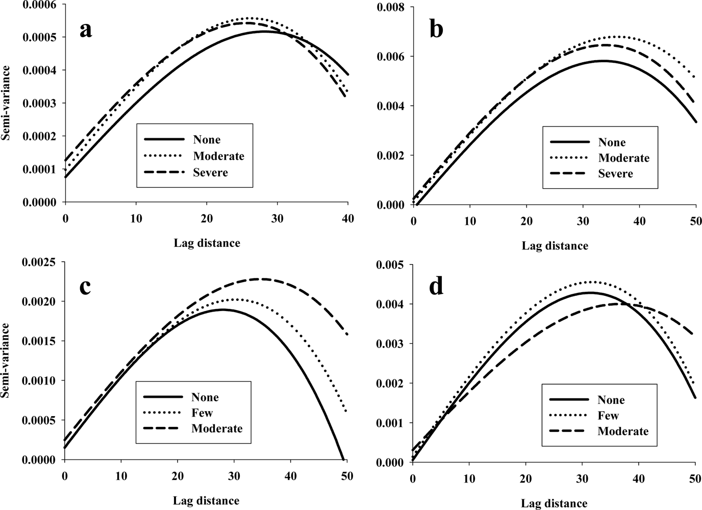
For each of the 480 combinations of spectral bands and variogram parameters (160 spectral bands × 3 variogram parameters), the relative effects of data set, maize hybrid, abiotic stress (irrigation regime), and biotic stress (spider mite infestation) were examined. The main purpose was to identify combinations of spectral bands and variogram parameters that could be considered reliable/unique stress indicators without showing significant response to difference between maize hybrids and/or between the 2 data sets. Several important observations could be made from this initial analysis (Figure 2): (1) most of the combinations of spectral bands and variogram parameters were found unsuitable as stress indicators mainly because of significant difference between the 2 data sets, especially in analyses of sill values, (2) nugget values (Figure 2(a)) from 645–675 nm and 766–826 nm (multiple spectral bands in each spectral range) responded significantly to abiotic stress without responding significantly to other treatment factors, (3) sill values (Figure 2(b)) showed a highly consistent response to biotic stress in spectral bands from 592 to 668 nm, but the same spectral bands also responded significantly to difference between data sets, so they were not considered further, (4) range values (Figure 2(c)) from 579 to 661 nm (multiple spectral bands) responded significantly to abiotic stress without responding significantly to other treatment factors, and (5) range values at 715 nm responded significantly to biotic stress without responding significantly to other treatment factors. Thus, it was demonstrated that there is considerable variation in the stress response by variogram parameters derived from different spectral bands, and that unique responses to abiotic and biotic stressors could be detected. It is suspected that more spectral bands responding significantly to abiotic stress than to biotic stress because the range of abiotic stress was likely wider than that of biotic stress. Variogram parameters derived from several of spectral bands near 700 nm responded significantly to the imposed stressors, so the data analysis presented here corroborate findings published elsewhere [4,8]. Based on results presented in Figure 2 and identification of highest F-values from all 480 analyses of variance, 4 spectral bands, (683 and 775 nm as abiotic stress indicators and 715 and 731 nm as biotic stress indicators) were selected for further analyses (Figure 3). It was seen that there was an increase in both nugget and sill values at 683 nm (Figure 3(a)) and 775 (Figure 3(b)) and that range values at 683 nm decreased in response to abiotic stress. Regarding variograms at 731 nm (Figure 3(c)) and 715 nm (Figure 3(d)), it was seen that range values increased in response to biotic stress, and sill values at 731 nm increased considerably.
Analysis of variance was used to identify statistical differences in variogram parameters in response to the imposed stressors (Figure 4). Figures 4a and b suggested that nugget values at 683 nm (Figure 4(a)) and 775 nm (Figure 4(b)) increased significantly when maize plants are subjected to severe drought stress compared to maize plants without drought stress. Regarding detection of biotic stress, nugget values at 731 nm (Figure 4(c)) and range values at 715 nm (Figure 4(d)) also showed significant responses.
4.2. Relationship between Reflectance Data and Variogram Parameters
Table 2 shows that none of the examined descriptive statistics revealed trends consistent with the identified variogram parameter responses, and that none of them could be considered reliable stress indicators. Thus, the findings in this study are not in agreement with Carter and Knapp [8], who, based on an extensive review, concluded that most plant stressors induce an increase in reflectance, especially in spectral bands near 700 nm. One possible explanation for the discrepancy between the results presented in this study and those by Carter and Knapp [8] is that this study was based on a heterogeneous composite of 2 data sets and 4 treatment factors (data set, maize hybrids, abiotic and biotic stressors). Furthermore, it is important to mention that spider mite infestation levels were generally low with highest count on a single maize plant equal to about 700 spider mites. Based on sampling of spider mite infested maize plants from greenhouse cultures and field plots, over 300 spider mites may be found on single maize leaves [23], which may amount to several thousand spider mites on a single plant (a fully developed maize plant typically has 15–20 leaves). Thus even though abiotic stress was referred to as ranging from “none” to “severe”, and biotic stress ranged from “none” to “moderate”, the imposed stress levels were quite subtle.
This low spider mite infestation level was intentional, as the objective was to test variogram based analysis on a challenging model system, and variogram parameters did respond significantly despite the fact that analysis of average reflectance values in the same spectral bands yielded no consistent trends. A recent study involving experimental manipulation of reflectance data (adding 2.5% or 5.0% to reflectance values in all or random subsets of pixels) showed that increase in reflectance especially affected sill values and to some extent also effected nugget values but had negligible effect on range values [24]. Thus, if mainly sill values respond to increases in reflectance values, it is not surprising that this study showed negligible increase in average reflectance and non-consistent response by sill values to the 2 stressors.
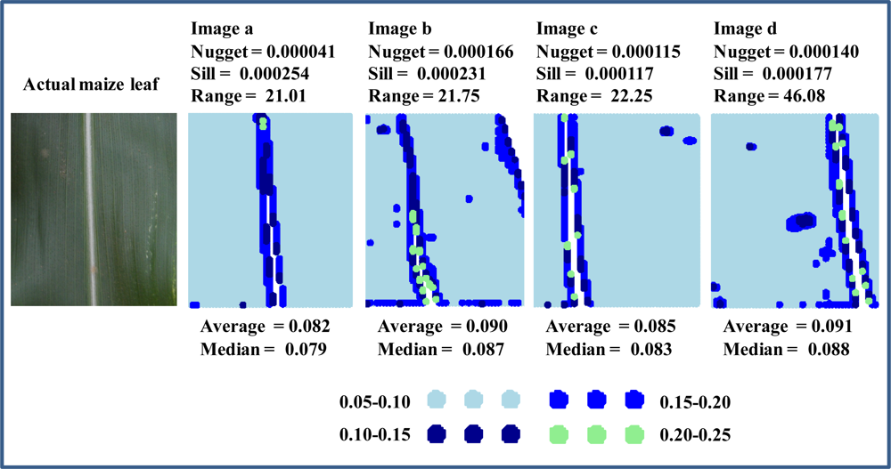
Without significant increase in average reflectance and/or width of 95% confidence limits, a remaining objective was to characterize the spatial distribution (scattering) of reflectance responses to imposed stressors. In this context, it is very important to mention that crop leaves are “never clean”—that dust, pollen, and discolorations will invariably be present, and they can obviously compromise classification accuracy of reflectance based approaches. Figure 5 shows a typical maize leaf image and 4 hyperspectral image files, which were selected based on their nugget and range values derived from the spectral band at 683 nm. Average reflectance values varied within 10% (0.82–0.91) with the vast majority of pixels having reflectance values between 0.05 and 0.10, and all 4 images were acquired near the leaf mid rib (white line of excluded pixels in the middle of each image). Comparing images a and b, it is seen that mainly due to a single large “spots” of increased reflectance in the top right corner caused a 4-fold increase in nugget values, while sill and range values remained fairly constant. Comparing images c and d, it is seen that a few scattered “spots” of increased reflectance caused a 2-fold increase in range values, while these scattered spots had negligible effect on nugget and sill values. The subtle variation in reflectance values among these 4 images emphasize the marked sensitivity of variogram analysis and how it may be used to amplify variations in data spatially organized data sets, which otherwise could not be differentiated.
Based on the findings in this study and results published elsewhere, it is hypothesized that if an imposed stress level is sufficiently high, it will lead to a significant increase in average reflectance, especially near 700 nm, and especially sill values will respond to such an increase [4,8]. However, even before a significant increase in average reflectance, stress expression in crop leaves may predominantly consist of scattered increases in reflectance within a given leaf, and that may lead to significant increases in both nugget and range values. In a theoretical model analysis of the relationship between chlorophyll distribution and leaf reflectance, Barton [25] concluded that: (1) Even small and subtle stress signs of chlorosis can significantly influence the reflectance of a leaf and that sensitivity of reflectance to chlorosis varies with wavelength. (2) Within-leaf variation in chlorophyll concentration due to stressors may markedly increase leaf reflectance and lead to underestimation of chlorophyll concentration. In addition, Barton [25] highlighted the importance of studying plant stress response based on individual leaves and also to incorporate spatial distribution information into the analysis.
5. Conclusions
This study confirmed results from previously published studies [4,8], that analysis of reflectance data near 700 nm show a strong stress response, but it was also shown that this spectral region may not be suitable for stress detection, when crop plants are subjected to more than 1 stressor and when other treatment factors are included in the analysis. With focus on variogram parameters, it was shown that especially nugget and range values increased significantly in response to the imposed stressors. Nugget values at 683 and 775 nm responded significantly to abiotic stress, and nugget values at 731 nm and range values at 715 nm responded significantly to biotic stress. Based on qualitative characterization of actual images, it was seen that even subtle changes in spatial patterns of reflectance values can elicit several-fold changes in variogram parameters despite non-significant changes in average and median reflectance values and in width of 95% confidence limits. Furthermore, it was hypothesized that, rather than causing a gradual increase in reflectance in all pixels, emerging plant stress expression predominantly elicit increases in reflectance in scattered pixels within a crop leaf. Such scattered stress expression is in accordance with documented within-leaf variation in both mineral content and chlorophyll concentration and therefore supports the need for reflectance-based stress detection at a high spatial resolution (many hyperspectral reflectance profiles acquired from a single leaf) and may be used to explain or characterize within-leaf foraging patterns of herbivorous arthropods.
Acknowledgments
This study was partially funded by the Texas Corn Producers Board.
References
- Reisig, D.; Godfrey, L. Spectral response of cotton aphid- (Homoptera: Aphididae) and spider mite- (Acari: Tetranychidae) infested cotton: Controlled studies. Environ. Entomol 2007, 36, 1466–1474. [Google Scholar]
- Delalieux, S.; Auwerkerken, A.; Verstraeten, W.W.; Ben Somers, B.; Valcke, R.; Lhermitte, S.; Keulemans, J.; Coppin, P. Hyperspectral reflectance and fluorescence imaging to detect scab induced stress in apple leaves. Remote Sens 2009, 1, 858–874. [Google Scholar]
- Nansen, C.; Sidumo, A.J.; Capareda, S. Variogram analysis of hyperspectral data analysis to characterize impact of biotic and abiotic stress of maize plants and to estimate biofuel potential. Appl. Spect 2010, 64, 627–636. [Google Scholar]
- Nansen, C.; Macedo, T.; Swanson, R.; Weaver, D.K. Use of spatial structure analysis of hyperspectral data cubes for detection of insect-induced stress in wheat plants. Int. J. Remote Sens 2009, 30, 2447–2464. [Google Scholar]
- Naumann, J.C.; Young, D.R.; Anderson, J.E. Spatial variations in salinity stress across a coastal landscape using vegetation indices derived from hyperspectral imagery. Plant Ecol 2009, 202, 285–297. [Google Scholar]
- Borzuchowski, J.; Schulz, K. Retrieval of leaf area index (LAI) and soil water content (WC) using hyperspectral remote sensing under controlled glass house conditions for spring barley and sugar beet. Remote Sens 2010, 2, 1702–1721. [Google Scholar]
- Kim, Y.; Glenn, D.M.; Park, J.; Ngugi, H.K.; Lehman, B.L. Hyperspectral image analysis for water stress detection of apple trees. Comput. Electron. Agr 2011, 77, 155–160. [Google Scholar]
- Carter, G.A.; Knapp, A.K. Leaf optical properties in higher plants: Linking spectral characteristics to stress and chlorophyll concentration. Am. J. Bot 2001, 88, 677–684. [Google Scholar]
- Jiménez, S.; Morales, F.; Abadía, A.; Abadía, J.; Moreno, M.A.; Gogorcena, Y. Elemental 2-D mapping and changes in leaf iron and chlorophyll in response to iron re-supply in iron-deficient GF 677 peach-almond hybrid. Plant Soil 2009, 315, 93–106. [Google Scholar]
- Uddling, J.; Gelang-Alfredsson, J.; Piikki, K.; Pleijel, H. Evaluating the relationship between leaf chlorophyll concentration and SPAD-502 chlorophyll meter readings. Photosynth. Res 2007, 91, 37–46. [Google Scholar]
- Neto, A.L.A.; Brunelli, H.C.; Fagan, R.; Dionisio, A.; Santos, B.M.; Tardivo, J.C.; Mariconi, F.A.M.; Franco, J.F. Two-spotted spider mite on cotton Tetranychus urticae Koch, 1836 and an experiment on its chemical control. Anais Soc. Entomol. Brasil 1978, 7, 133–139. [Google Scholar]
- Stiefel, V.L.; Margolies, D.C.; Bramel-Cox, P.J. Leaf temperature affects resistance to the Banks grass mite (Acari: Tetranychidae) on drought-resistant grain sorghum. J. Econ. Entomol 1992, 85, 2170–2184. [Google Scholar]
- Toole, J.L.; Norman, J.M.; Holtzer, T.O.; Perring, T.M. Simulating Banks grass mite (Acari: Tetranychidae) population dynamics as a subsystem of a crop canopy-microenvironment model. Environ. Entomol. 1984, 13, 329–337. [Google Scholar]
- Perring, T.M.; Holtzer, T.O.; Toole, J.L.; Norman, J.M. Relationships between corn-canopy microenvironments and Banks grass mite (Acari: Tetranychidae) abundance. Environ. Entomol 1986, 15, 79–83. [Google Scholar]
- Feese, H.; Wilde, G. Factors affecting survival and reproduction of the Banks grass mite, Oligonychus pratensis. Environ. Entomol 1977, 6, 53–56. [Google Scholar]
- Nansen, C. Robustness of analyses of imaging data. Opt. Express 2011, 19, 15173–15180. [Google Scholar]
- Armstrong, M. Basics of Semi-Variogram Analysis; Springer: Berlin, Germany, 1998. [Google Scholar]
- Isaaks, E.H.; Srivastava, R.M. Applied Geostatistics; Oxford University Press: New York, NY, USA, 1989. [Google Scholar]
- Liebhold, A.M.; Rossi, R.E.; Kemp, W.P. Geostatistics and geographic information systems in applied insect ecology. Ann. Rev. Entomol 1993, 38, 303–327. [Google Scholar]
- Rossi, R.E.; Mulla, D.J.; Journel, A.G.; Franz, E.H. Geostatistical tools for modeling and interpreting ecological spatial dependence. Ecol. Monogr 1992, 62, 277–314. [Google Scholar]
- Krajewski, S.A.; Gibbs, B.L. Understanding Contouring. A Practical Guide to Spatial Estimation Using a Computer and Semi-Variogram Interpretation; Gibbs Associates: Boulder, CO, USA, 2001. [Google Scholar]
- Bohling, G. Introduction to Geostatistics and Semi-Variogram Analysis. 2005. Available online: http://people.ku.edu/~gbohling/cpe940 (accessed on 25 October 2011).
- Nansen, C.; Sidumo, A.J.; Gharalari, A.H.; Vaughn, K. A new method for sampling spider mites on field crops. Southwest. Entomol 2010, 35, 1–10. [Google Scholar]
- Nansen, C.; Abidi, N.; Sidumo, A.J.; Gharalari, A.H. Using spatial structure analysis of hyperspectral imaging data and fourier transformed infrared analysis to determine bioactivity of surface pesticide treatment. Remote Sens 2010, 2, 908–925. [Google Scholar]
- Barton, C.V. A theoretical analysis of the influence of heterogeneity in chlorophyll distribution on leaf reflectance. Tree Phys 2001, 21, 789–795. [Google Scholar]
Figure 1.
Basic description of variogram analysis applied to reflectance data.

Figure 2.
Analysis of variance of nugget (a), sill (b) and range (c) values in 160 spectral bands between 405 and 907 nm in response to 4 treatment factors: (1) difference between data set 1 and 2 (Table 1), (2) difference between hybrid 1 and 2, (3) response to abiotic stress, and (4) response to biotic stress. Horizontal bars represent spectral regions with significant response to either abiotic (dashed) or biotic (non-dashed) stressor at the 0.05-level.

Figure 3.
Variograms of reflectance data at 683 nm (a) and 775 (b) in response to abiotic stress, and at 731 nm (c) and 715 nm (d) in response to biotic stress.
Figure 3.
Variograms of reflectance data at 683 nm (a) and 775 (b) in response to abiotic stress, and at 731 nm (c) and 715 nm (d) in response to biotic stress.

Figure 4.
Nugget values at 683 nm (a) and 775 (b) in response to abiotic stress, and nugget values at 731 nm (c) and range values at 715 nm (d) in response to biotic stress. Different letters denote statistical difference at the 0.05-level.
Figure 4.
Nugget values at 683 nm (a) and 775 (b) in response to abiotic stress, and nugget values at 731 nm (c) and range values at 715 nm (d) in response to biotic stress. Different letters denote statistical difference at the 0.05-level.

Figure 5.
Maize leaf images: an actual RGB image and 4 images based on reflectance values at 683 nm with each image representing 10,000 pixels.
Figure 5.
Maize leaf images: an actual RGB image and 4 images based on reflectance values at 683 nm with each image representing 10,000 pixels.


| DAI | Non-Infested | Infested | ||||||
|---|---|---|---|---|---|---|---|---|
| None | Moderate | High | None | Moderate | High | |||
| Data set 1 | 8 Dec | 3.00 | 6 | 6 | 6 | 6 | 6 | 6 |
| 12 Dec | 7.00 | 6 | 6 | 6 | 6 | 6 | 6 | |
| 14 Dec | 9.00 | 6 | 6 | 6 | 6 | 6 | 6 | |
| Data set 2 | 28 Mar | 3.00 | 5 | 5 | 6 | 4 | 5 | 6 |
| 31 Mar | 6.00 | 5 | 5 | 6 | 4 | 5 | 6 | |
| 2 Apr | 8.00 | 5 | 5 | 6 | 4 | 5 | 5 | |
| 5 Apr | 10.00 | 5 | 5 | 6 | 4 | 4 | 5 | |
“DAI” denotes days after infestation of maize plants with spider mites, and non-infested/infested refers to whether the maize plants were infested with spider mites.
| Average | Median | Standard Error | Lower | Confidence Limits | ||
|---|---|---|---|---|---|---|
| Upper | Width | |||||
| Response to abiotic stress at 683 nm | ||||||
| None | 0.091ab | 0.087ab | 0.000030 | 0.090 | 0.091 | 0.000118 |
| Moderate | 0.089a | 0.083a | 0.000034 | 0.089 | 0.089 | 0.000132 |
| High | 0.093b | 0.088b | 0.000035 | 0.093 | 0.093 | 0.000136 |
| Response to abiotic stress at 775 nm | ||||||
| None | 0.836ab | 0.840ab | 0.000121 | 0.836 | 0.836 | 0.000474 |
| Moderate | 0.823a | 0.825a | 0.000137 | 0.823 | 0.824 | 0.000539 |
| High | 0.856b | 0.859b | 0.000132 | 0.856 | 0.856 | 0.000519 |
| Response to biotic stress at 715 nm | ||||||
| None | 0.370 | 0.366 | 0.000084 | 0.370 | 0.370 | 0.000331 |
| Few | 0.372 | 0.371 | 0.000087 | 0.372 | 0.373 | 0.000341 |
| Moderate | 0.389 | 0.386 | 0.000129 | 0.389 | 0.389 | 0.000504 |
| Response to biotic stress at 731 nm | ||||||
| None | 0.638ab | 0.640ab | 0.000088 | 0.638 | 0.638 | 0.000345 |
| Few | 0.633a | 0.639a | 0.000098 | 0.633 | 0.634 | 0.000385 |
| Moderate | 0.66b4 | 0.663b | 0.000148 | 0.664 | 0.664 | 0.000581 |
Different letters across stress levels (vertical comparison) denote difference at the 0.05-level.
Share and Cite
MDPI and ACS Style
Nansen, C. Use of Variogram Parameters in Analysis of Hyperspectral Imaging Data Acquired from Dual-Stressed Crop Leaves. Remote Sens. 2012, 4, 180-193. https://0-doi-org.brum.beds.ac.uk/10.3390/rs4010180
AMA Style
Nansen C. Use of Variogram Parameters in Analysis of Hyperspectral Imaging Data Acquired from Dual-Stressed Crop Leaves. Remote Sensing. 2012; 4(1):180-193. https://0-doi-org.brum.beds.ac.uk/10.3390/rs4010180
Chicago/Turabian StyleNansen, Christian. 2012. "Use of Variogram Parameters in Analysis of Hyperspectral Imaging Data Acquired from Dual-Stressed Crop Leaves" Remote Sensing 4, no. 1: 180-193. https://0-doi-org.brum.beds.ac.uk/10.3390/rs4010180