An International Comparison of Individual Tree Detection and Extraction Using Airborne Laser Scanning

Abstract

The objective of the “Tree Extraction” project organized by EuroSDR (European Spatial data Research) and ISPRS (International Society of Photogrammetry and Remote Sensing) was to evaluate the quality, accuracy, and feasibility of automatic tree extraction methods, mainly based on laser scanner data. In the final report of the project, Kaartinen and Hyyppä (2008) reported a high variation in the quality of the published methods under boreal forest conditions and with varying laser point densities. This paper summarizes the findings beyond the final report after analyzing the results obtained in different tree height classes. Omission/Commission statistics as well as neighborhood relations are taken into account. Additionally, four automatic tree detection and extraction techniques were added to the test. Several methods in this experiment were superior to manual processing in the dominant, co-dominant and suppressed tree storeys. In general, as expected, the taller the tree, the better the location accuracy. The accuracy of tree height, after removing gross errors, was better than 0.5 m in all tree height classes with the best methods investigated in this experiment. For forest inventory, minimum curvature-based tree detection accompanied by point cloud-based cluster detection for suppressed trees is a solution that deserves attention in the future.

1. Introduction

The development of laser/radar ranging measurements without scanning and proper attitude control for forest inventory in 1970s–1990s [1–11] promoted the application of laser measurement in forestry and led to the rapid adaptation of airborne laser scanning (ALS) in forest inventory. At first, ALS was applied in determining forest terrain elevations [12,13]. This was immediately followed by standwise mean height and volume estimation [14–16], based on the data collected via ranging measurements, and very soon ALS was applied to inventorying, focusing on individual trees [17–20] with the advent of rapid image processing, tree species classification [21,22] and the measurement of tree growth and detection of harvested trees [23] based on bi-temporal data sets. Over 10 years, the extraction of forest variables has been divided into two categories: area-based inventories and inventories based on individual trees or groups of trees. Concurrently with these developments, laser scanning has increasingly provided the core data set for mapping authorities. The point density of laser scanning has increased constantly. In addition to being used in forest inventory, ALS data from forested areas is used for purposes such as flight obstacle mapping, power line mapping, virtual city visualization and mapping, and telecommunication planning.

In the Nordic countries the retrieval of stand characteristics (e.g., mean tree height, dominant height, mean diameter, stem number, basal area, and timber volume), which are needed in forest management planning, is currently being replaced by ALS-based inventory methodologies. As regards operational forest inventories, the two-stage procedure using ALS data and field plots, i.e., area-based approach (ABA, [24]), has become common and a reference for other inventory methodologies. The foremost advantages of the state-of-the-art ABA, when compared to traditional standwise field inventory (SWFI), are greater precision in the prediction of forest variables [25], sampling-based estimation of forest variables with the possibility to calculate accuracy statistics, and (at least in principle) ALS-based inventory is not dependent on stand boundaries. Moreover, current ALS data acquisition and processing costs are less than those of traditional SWFI methods.

The ALS-based forest inventory methodology based on individual tree detection (ITD) has been widely studied recently, but is not widely used in practice, due to assumed problems related to tree detection under various forest conditions [26–28]. Other problems related to the practical use of ITD include the need for higher ALS point density, which adds to the costs and the amount of data that would need to be stored, as well as inadequate tree species identification accuracy. The assumed main advantage of ITD would be that it provides true stem distribution series, enabling better predictions of timber assortments. Stem distributions are predicted in the ABA, causing inaccuracy in timber assortment estimates and forest value [29]. Another advantage of ITD is the reduced amount of expensive fieldwork compared to that needed when applying the ABA approach.

The results obtained for individual tree extraction have varied significantly from study to study. Percentage of correctly delineated trees has ranged from 40% to 93%, [17,21,29–36]. It was not known how much of this variation was caused by the methods and how much by forest conditions, until the international benchmarking study “Tree Extraction” (2005–2008) was carried out. In order to test the tree extraction methods using the same data sets, the European Spatial Data Research Organization (EuroSDR) and the International Society for Photogrammetry and Remote Sensing (ISPRS) initiated the “Tree Extraction” project to evaluate the quality, accuracy, and feasibility of automated tree extraction methods based on airborne laser scanner data and digital aerial images. The project was hosted by the Finnish Geodetic Institute (FGI). Twelve partners from USA, Canada, Norway, Sweden, Finland, Germany, Austria, Switzerland, Italy, Poland and Taiwan participated in the test included in the “Tree Extraction” project. The partners were requested to extract trees using the given ALS and image datasets. Another objective of the study was to find out how the point density impacts on individual tree extraction. The results were published in the project’s final report [27]. The report sets out the accuracy of tree extraction per partner, but it does not present a more detailed analysis of the results. The final report showed that the extraction method is the main factor affecting achieved accuracy. When the laser point density increased from 2 points to 8 points per m², the improvement in crown delineation accuracy was marginal.

Tree detection accuracy results from heterogeneous forests are presented in Pitkänen et al. [37] where the detection accuracy was only 40% (70% for dominant trees). Yu et al. [38] presented an accuracy of 69% for tree detection under various forest conditions (different forest densities, ages, site types and tree species). Heinzel et al. [39] introduced an approach that classifies crown size in advance and uses this information as prior knowledge for single-tree extraction. Crown size is classified from aerial color infrared image texture with an improved grey-scale granulometry followed by a crown size adapted watershed segmentation of single trees. The accuracy varies between 64% and 88%. Vauhkonen et al. [40] tested several algorithms under different types of forests; Eucalyptus plantation in Brazil, coniferous and deciduous plots in Germany and mainly coniferous plots in Norway and in Sweden. The tree detection rate varied between 54% and 86%. These results are on a completely different scale from those obtained by Peuhkurinen et al. [41], where ITD was carried out in two marked stands (density ∼465 stems per ha). The number of harvestable trees was underestimated by only <3%, but this result may include some commission errors, i.e., a single tree is segmented into several segments, thus increasing the number of detected trees. Falkowski et al. [42] showed that across a full range of canopy conditions in a mixed-species, structurally diverse conifer forest in northern Idaho, United States, the effect of the canopy cover density is significant for tree detection accuracy. Vastaranta et al. [43] combined automated ITD and visual interpretation to acquire reference data for ABA. They assumed that additional visual interpretation would significantly enhance the accuracy of the derived plot-level forest variables and provide superior results when used to train the ABA, in contrast to mere automated ITD. Visual interpretation improved the accuracy of ITD validated at plot-level as RMSE of stem volume decreased from 32.1% to 28.6%. However, there was no improvement in ABA predictions.

Vastaranta et al. [28] investigated ITD error sources, and their effects on forest management planning calculations. The investigated error sources were detection of trees, errors in tree height prediction and errors in tree diameter prediction. The effects of these errors were analyzed with Monte Carlo simulations. The results showed that the foremost error source in ITD is in tree detection.

This paper includes further analyses of the results obtained in the “Tree Extraction” project [27]. Four additional methods were added for comparison, namely (1) Local maxima (LM) finding, (2) Multi-scale Laplacian of Gaussian, (3) Minimum curvature-based tree detection and (4) LM finding with varying window size. The LM finding method is a relatively easy and fast implementation, ready for operational use, and advanced methods should provide better results. Additionally, the results are analyzed for various tree heights, and omission and commission errors were included. Finally, more conclusions are drawn from the experiment’s results.

Section 2 describes the data sets used in the study. Section 3 provides a brief description of the methods used by the partners and of the methods used for the evaluation. Section 4 presents the results for the evaluated parameters and discussion. The accuracy of tree height and location determination, crown delineation and the number of extracted trees are analyzed. Key conclusions are given in Section 5.

2. Material

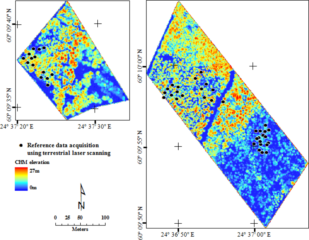
2.1. Study Area

The selected two managed forest test sites, named Site A and Site B (Figure 1), were close to each other in Southern Finland, about 18 km west of Helsinki. Test sites were very diverse, partly flat and partly steep terrain (max elevation difference 45 m), with patches of mixed and more homogeneous tree species in various stages of development. The main tree species on the two sites were Scots pine (Pinus sylvestris), Norway spruce (Picea abies) and Silver and Downy birches (Betula sp.). Site A was 2.6 ha and Site B 5.8 ha in size.

2.2. Data Provided for Tree Extraction

ALS data (

Table 1. ALS data collected from the study sites.

Acquisition	29 June 2004
Instrument	Optech ALTM 2033
Flight altitude	600 m
Pulse frequency	33,000 Hz
Field of View	±9 degrees
Measurement density	2 points per m2 per echo per strip
Swath width	185 m
Mode	First and last pulse

) with three point densities (2, 4 and 8 points per m²) was provided to the partners. A digital terrain model (DTM) with 0.5m grid spacing was calculated using the TerraScan-software (algorithm based on Axelsson [44]) and delivered as ASCII-grid. The training dataset was measured with a total station and included species, location, diameter at breast height (DBH), and crown delineation (using 3–5 points per crown) of 75 trees.

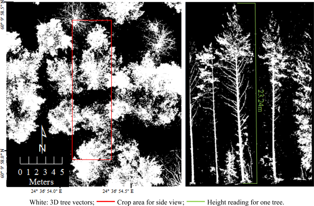
2.3. Reference Data

The reference data were collected by means of ground surveys and terrestrial laser scanning (TLS). RTK–GPS (Leica SR530) and total station (Trimble 5602S DR200+) equipment were used to create a network of ground control points (GCP) over the study sites. The 3D accuracy of the GCP’s was estimated to be 2–3 cm, which could be verified by repeated RTK-GPS measurements (accuracy 1 cm + 1–2 ppm in plane and 1.5–2 cm + 2 ppm in height [45]) and total station observations. The locations of spherical reference targets for a terrestrial laser scanner (Faro LS880HE) were determined with reference to total station measurements on the basis of the GCPs. Terrestrial laser scanning was carried out in 48 locations (Figure 1) to obtain laser point coverage of all reference trees on five test plots, two plots on Site A and three plots on Site B. Together the five plots covered an area of 0.48 ha (5.7% of total test site area). The reference data included the locations and species of 352 trees and the heights of 254 trees (

Table 2. Reference data tree species distribution and heights.

Species	%	Tree Height (m)
		Mean	Max.	Std.
Scots pine	20	11.2	22.9	7.3
Norway spruce	46	14.2	25.5	6.7
Birch	15	20.3	27.2	5.3
Other deciduous	19	10.2	25.6	7.1

).

The point clouds of the individual terrestrial laser scannings were georeferenced using spherical reference targets. Then each point cloud was triangulated into a 3D-mesh. The 3D vectors of individual scannings were combined (Figure 2), and tree parameters were measured manually using 3D CAD software. The measured tree parameters included tree trunk location, tree top location, tree height, and crown delineation. Tree heights were measured only for trees that had the tree top clearly visible in the data. Crown delineation was analyzed as crown covered area, so individual crowns were not separated on denser areas. The intensity images of the original scannings were used to determine tree species.

2.4. Produced Tree Extraction Results

The partners were requested to extract trees using the given material. They were free to use any method. The partners were asked to provide the tree locations and heights, crown delineations, and heights of the crown base or the volumes for each tree that they could extract. Nine out of the twelve partners in the “Tree Extraction” project used solely laser scanning data and were included in this comparison. Two partners used both laser scanning data and airborne images and one used solely airborne images.

3. Methods

3.1. Methods Used by the Partners

The methods (

Table 3. Method names and partners.

Method	Partner	Country
Definiens	Definiens AG	Germany
FOI	Swedish Defense Research Agency	Sweden
Hannover	Leibniz Universität Hannover	Germany
Metla	Finnish Forest Research Institute	Finland
Norway	Norwegian Forest and Landscape Institute and Norwegian University of Life Sciences	Norway
Ilan	National I-Lan University	Taiwan
Texas	Texas A&M University	USA
Udine	University of Udine	Italy
Zürich	University of Zürich	Switzerland

) have been reported in detail in Kaartinen and Hyyppä [27]. Here, a brief description of the key elements of the methods is provided.

3.1.1. Method Definiens

Method Definiens was implemented in eCognition Expert software using the point density of 8 points per m². The method may be divided into four main tasks: (1) Creation of a forest mask, (2) Initial splitting of the forest mask, (3) Splitting the forest mask into tree crowns and (4) Correction of over-split crowns. A low-pass filter was applied to remove small gaps and excessive local minima and maxima. The creation of the forest mask was performed by thresholding the canopy height model (CHM) images at the height of 2 m. CHM is computed as the difference between DTM and digital surface model (DSM). The method used the highest point/pixel in the object as the seed and expands the seed to the crown boundaries, which were identified by the positive difference between the current and the proposed pixel. This was repeated until all areas within the current object had been included into new objects. The difference required to form a boundary was defined with a threshold. The threshold was initially high and a boundary was formed only where a large difference occurs, in this case at 1 m. The key to this method is the classification of objects into two groups, crowns and crown-clusters. Those objects identified as crowns were removed from further splitting iterations and only considered later, while crown-clusters were processed further in the hope of separating the crowns contained within them.

3.1.2. Method FOI

Method FOI was fully automated and had the following steps: (1) DSM creation, (2) DTM creation, (3) CHM creation, (4) CHM filtering using different Gaussian filters resulting in different images, (5) Segmenting of the different images separately and selecting the segment chosen for a specific area by fitting a parabolic surface to the laser data, (6) Estimation of the heights and crown diameters of the identified trees using the elevation data and the area of the segment [30]. The method works on gridded data, in this case 0.25 m × 0.25 m.

3.1.3. Method Hannover

Method Hannover was based on a tree model with three geometric parameters (size, circularity and convexity of the tree crown). The processing strategy comprised four steps. First, a wide range of DSM scale levels was created. The second step was segmentation, achieved by applying a watershed transformation. In the third step, the best hypothesis for a crown from the overlapping segments of all levels based on the tree model was selected. The selection of the best hypotheses was achieved with the help of fuzzy functions for the tree model parameters [46].

3.1.4. Method Metla

In Method Metla, a DSM pixel was considered to be a low, differing pixel, if at least seven (surface models from point density of eight points per m²), or six (other point densities) of the eight nearest neighbors were more than five meters higher than the pixel itself. These pixels were replaced with the median of the more-than-five-meters-larger neighbor pixel values. The DTM was then subtracted from the final DSM to get the CHM for the tree crown segmentation. Before segmentation, the CHM was smoothed with height-based filtering. Five Gaussian filters were used so that the filter size increased along the height of the pixel being smoothed. The minimum and maximum σ values were selected by visually ensuring that the number of LM was reasonable at both ends of the tree height range. A negative image of the height-filtered image was then created for watershed segmentation that was used to separate the tree crowns from each other. Watershed regions associated with the local minima in the negative image were identified using an algorithm following the drainage direction. To determine the boundaries between crowns and background, pixels lower than 2 m in the height-filtered image were masked out from the crown segments. Finally, small segments (at most three pixels in size) were combined with one of the neighbor segments, this being a tree crown or the background, based on the smallest average gradient on the common segment boundary. The tree locations and heights were then obtained from the location and the value of the pixel having the highest value within each segment.

3.1.5. Method Norway

In Method Norway, the process was comprised of several steps, i.e., retain uppermost echoes, interpolate them into a DSM-grid, find LM in the DSM, run a region-growing algorithm with some restrictions in order to derive objects belonging to the class of objects often named star objects. The DSM was now divided into segments that represented tree crowns, while parts of the area were not covered by trees and had no DSM value. The DSM was adjusted (lifted) using the residuals between the DSM and the first echoes. The 90 percentile of the residuals was calculated, and this frequently turned out to be around 70 cm. This offset was added to all z values in the DSM. The tree heights were derived as the z value of the LM after this adjustment [47].

3.1.6. Method Ilan

In Method Ilan, the tree locations and tree height were computed from the CHM. The CHM was computed by selecting the highest laser point within each 1 m × 1 m grid cell. Furthermore, each trunk of the training dataset was located within a 3 m × 3 m window, and a height histogram with one-meter interval was used to build up a laser classification tree model for species determination. The highest laser echo within a specific area (i.e., 3 × 3 m), was assumed to be the potential trunk location of a tree. Two approaches were used to estimate the potential tree locations. The first approach involved running a LM filter in the CHM with a window size of 3 × 3, and all potential tree locations were selected. The second method processed only heights less than 15 m in the CHM with 3 × 3 LM filter. The first approach was applied to Site B, and the second approach was applied to Site A. The crown widths were derived, based on the training tree data (the relationship between tree species, tree height and crown width) and the CHM. The empirical relationship between the height of the trees and their searching crown size was defined.

3.1.7. Method Texas

Method Texas employed an automated algorithm of LM filter with a circular moving window of varying sizes. The algorithm was applied on CHMs with different pixel sizes depending on the point densities: 50 cm and 100 cm for 2 points per m², 50 cm for 4 points per m², and 25 cm and 50 cm for 8 points per m². The LM filter is often used to locate tree positions based on the assumption that the highest elevation corresponds to the tree apex. When applying the LM filter, the window size has a major impact on tree identification. On the other hand, it can be assumed that the taller a tree is, the larger is the width of its crown. Thus, determining the filter size was based on the relationship between crown size and tree height. Prior information was utilized to derive such a relationship. To predict the crown size, regression models were fitted with tree height as the independent variable. For the test data, about 90 trees on each site were visually identified from the CHMs and the corresponding heights and crown widths were manually recorded by means of on-screen measurement. The crown diameter was the average of two values measured along two perpendicular directions from the location of the tree top.

3.1.8. Method Udine

Method Udine consisted of the implementation of an algorithm that removes the points (ground and non-ground) derived from the echoes that penetrate inside the crown from the dataset. At first, the algorithm provided a triangulation of all the points. The following step was the removal of all the vertices that presented a difference greater than a fixed threshold. The procedure therefore allows a correct DSM to be obtained. The method applied in tree counting was based on a morphological analysis of the laser point distribution. For this purpose, the Top Hat algorithm was implemented. This is a mathematical function of image elaboration, which enables the top elements at the scale of the represented values to be found. The mathematical formulation of the Top Hat is related to the theory of image processing formulated by Serra [48,49]. In some cases, because of the presence of minor height variations among adjoining points belonging to the same crown, more than one apex may be counted for each tree. In order to minimize this kind of an error, a control algorithm was introduced. It detects and corrects erroneously classified apexes (these are often localized at the edge of the crown). In order to delineate single crowns, an algorithm for region growing was implemented.

3.1.9. Method Zürich

Method Zürich was based on LM detection in the CHM and a subsequent cluster analysis of the raw data with LM as the starting points. The DSM generation included a choice of four parameters, i.e., destination grid resolution, search radius, and the size and shape of a Gaussian smoothing function. The outcome of the cluster analysis was the raw data being flagged with a distinct number of all returns that were presumed to belong to a tree. This cluster was then treated by a routine, taking the relevant measures from the point cloud. These were the following:

• Position (x, y) was derived as the centre of gravity of the echo positions belonging to the cluster.
• Tree height was computed as the maximum height of the cluster’s echoes.
• Crown diameter was estimated using the convex hull of the cluster by transferring the circum-distance of the convex hull to a radius assuming circular shape.

3.1.10. Manually Extracted Trees (Manual)

The trees within the reference plots were also detected and extracted manually to compare the result of manual tree extraction with automated techniques. Extraction was executed using laser scanner data (8 points per m²) and TerraScan software. Additionally, aerial images (Vexcel UltraCam D, acquisition date 11 October 2004, ground sampling distance 20 cm) were used for interpretation purposes. The crown-covered areas were delineated visually on computer screen by using laser points (color-coded based on elevation), and the tree locations and heights were determined by finding the highest laser points within the delineated crowns. Ground elevation was interpreted visually from the 3D-view. The DTM was not used so that the whole process is fully manual. The results of this manual extraction are denoted as ‘Manual’.

3.2. Methods Added to the Test

In addition to these methods included in the EuroSDR comparison, four methods were implemented and tested by the FGI using the point density of 8 points per m². All four methods are based on CHM analysis. DSM was created by taking the highest laser hit in each grid cell of 0.5 m × 0.5 m. Also, DTM was provided in 0.5 m × 0.5 m grid.

3.2.1. Local Maxima Finding (FGI_LOCM)

Potential tree locations were found in the pre-filtering of the CHM by searching the LM in a given neighborhood. The filter used was a kernel of 3 × 3 window size with the following values:

$$\mathit{Kernel}=\frac{1}{28}\left[\begin{array}{ccc}1& 3& 1\\ 3& 12& 3\\ 1& 3& 1\end{array}\right]$$

(1)

Tree crowns were delineated using marker-controlled watershed transformation with the tree locations found in the previous step as control markers. The final tree locations and heights were then obtained from the location and value of the pixel having the highest value within each tree segment. If more than one pixel had the highest value, mean value was taken. The crown area was transformed into diameter by assuming a circular shape.

3.2.2. Multi-scale Laplacian of Gaussian (FGI_MLOG)

This method was based on the Laplacian of Gaussian operation (LoG), characterized by a scale factor. First, the CHM created in the first step of the procedure was smoothed with a Gaussian filter at a certain scale to yield a scale-space representation and then the Laplacian operator was computed. A multi-scale representation of images was obtained by choosing a different scale factor for LoG filter. This representation was necessary for capturing objects of different sizes. Scale factor selections were determined by the smallest and largest crown sizes. In order to select the best scale factor for representing different size objects in the view area, the Laplacian operator was replaced by a scale-normalized Laplacian operator. The tree locations were then detected by searching LM in the scale-space, i.e., those points that were simultaneously LM with respect to both space and scale or by searching the LM within the sum of images in different scales. Tree crowns were segmented using watershed. The background was masked out before crown segmentation by means of a thresholding operation; pixels lower than the given thresholds were filtered out. The final tree locations, heights and crown diameters were then obtained using the same procedure as in FGI_LOCM.

3.2.3. Minimum Curvature-Based Tree Detection (FGI_MCV)

This method was based on the minimum curvature computation of CHM. Minimum curvature, one of the two principal curvatures of a surface, is the curvature of a normal section with the smallest value of curvature among all normal sections at a given point on the surface. For a surface such as CHM, minimum curvature >0 describes the tree top, and minimum curvature <0 describes the valley between trees. The procedure consists of the following steps: first, CHM was created and filtered (e.g., using a Gaussian filter) and then the minimum curvatures were calculated. The CHM image was scaled by the created minimum curvature image and the LM were searched within a given neighborhood and used as markers in the following marker-controlled watershed transformation for tree crown delineations. The final tree locations, heights and crown diameters were then obtained using the same procedure as in FGI_LOCM.

3.2.4. Local Maxima Finding with Varying Window Size (FGI_VWS)

This method employed an automatic algorithm of LM finding with a moving window of varying sizes. In the detection of LM, the window size influences the tree identification greatly. It makes sense that LM is searched for within crown size area. Since tree height and crown size are closely interconnected, varying window size was determined from tree height. A previously derived model was utilized to predict the crown size, i.e., window size, which varied from pixel to pixel. Crown boundary, tree locations, heights and crown diameters were then obtained using the same procedure as in FGI_LOCM.

3.3. Methods Used for Evaluation

3.3.1. Automated Matching Between Reference Models and Provided Models

The accuracy of determining tree locations was evaluated by measuring the distances from every reference tree to the nearest tree found using the delivered model. The coordinates of the reference treetops were used in locating trees. Only distances within 5 m from the reference tree were included in the analysis. If several reference trees had hits on the same tree in the provided model, only the best match according to distance and height was accepted for inclusion in the analysis. The location accuracy was analyzed for all trees and for trees higher that 15 m (median height of reference trees was 14.5 m). The trees accepted for location accuracy evaluation were also used in evaluating tree heights, and again separately for all trees and for trees higher than 15 m. Tree location accuracy and height accuracy were also analyzed in five classes based on the reference tree heights: 2–5 m, 5–10 m, 10–15 m, 15–20 m and more than 20 m. Crown delineation accuracy was evaluated by comparing the total delineated area of reference trees to the provided model delineation. If a partner did not deliver crown delineation as vector data, the area covered by the crown was determined as a circular area around the trunk location by using the given radius or area, and the final delineated area was obtained as the union of these circles.

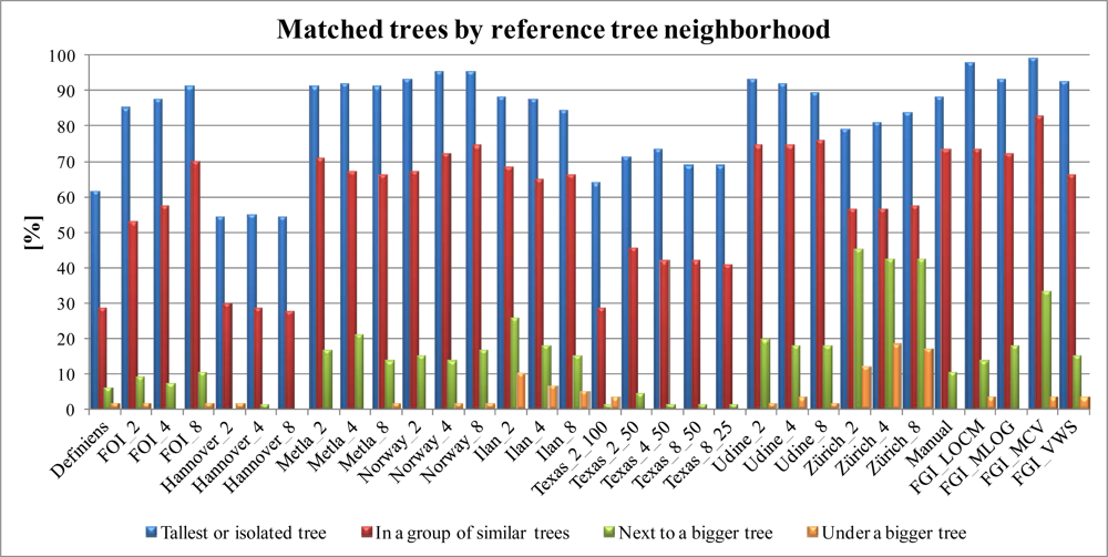
3.3.2. Impact of the Neighborhood

The impact of tree neighborhood on the performance of tree modeling was evaluated by first classifying the reference trees manually into four classes according to their location:

• Tallest tree in the neighborhood or isolated tree (neighbor distance in 2D over 3 m).
• Tree in a group of similar trees (neighbor within 3 m).
• Tree located next to a bigger tree.
• Tree under a bigger tree.

Classification into classes 3 and 4 was based on empirical observations both on site and during reference data processing. “Tree located next to a bigger tree” means that the tree in question is situated so that it is likely to be merged to its taller neighbor, for example in DSM computation. “Tree under a bigger tree” means that the tree is totally covered by its neighbor’s crown.

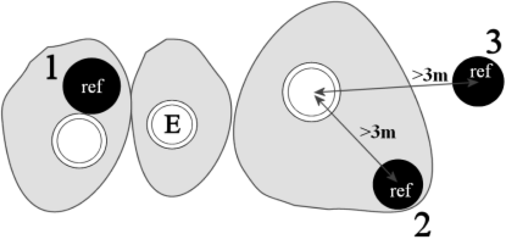
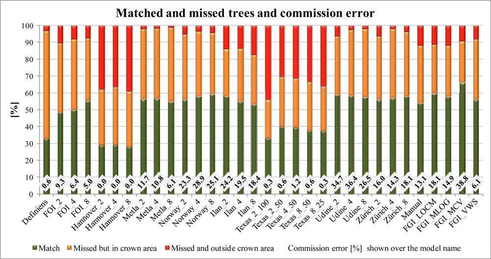
3.3.3. Matching Correctness and Commission and Omission Errors

Every reference tree was visually checked against the provided model and the results of the comparison were classified into three classes (Figure 3):

• A matching tree was found in the model (within a distance of 3 m and the height difference less than 5 m, depending on the tree height and surroundings).
• Matching tree was not found (according to the criteria above), but a reference tree was within the model crown area.
• Matching tree was not found (according to the criteria above) and a reference tree was outside the model crown area (omission error).

All trees at least 2 m in height in the provided model that did not have a match among the reference trees (ground truth) were marked. The number of the extra trees, i.e., the commission error, was computed. 2 m was selected as a threshold as most methods did not model smaller trees. In Class 1, the height threshold of 5 m was not strict. The classification was done manually and some subjectivity was allowed, based on the tree height and surroundings.

3.3.4. Treatment of Outliers

If the observed value differed from the reference value by more than the mean ±3 times the standard deviation, it was considered to be a gross error, or outlier, and it was deleted. When conducting tree height analysis, values deviating by more than 10 m from the ground truth were initially deleted.

4. Results and Discussion

The following figures show the laser point densities marked as per Method ID, e.g., FOI_2 for 2 points, FOI_4 for 4 points and FOI_8 for 8 points per m². In Method Texas’ results, the second number depicts the CHM pixel size in cm.

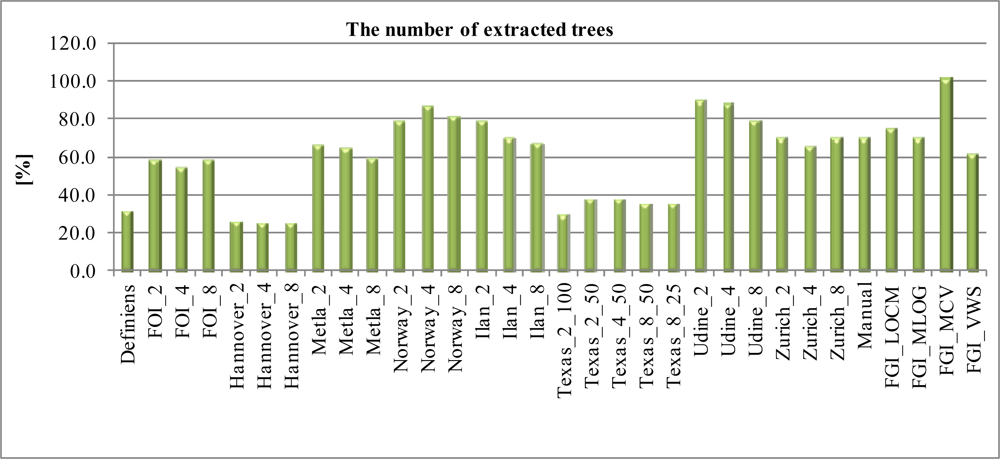
4.1. The Number of Extracted Trees

The number of extracted trees on the reference site plots is shown in Figure 4. This number reveals the percentage of the actual trees that have been extracted. In order to provide non-biased estimates, e.g., for volume, the correct percentage rate should be as high as possible without creating too many commission errors. The percentage of detected trees varies between 25% to 102%, implying different capabilities in detecting dominant and suppressed trees. Manual processing found 70% of the trees, which corresponds to the performance of one of the first automated tree extraction methods by Persson et al. [30]. Neighborhood information and omission and commission statistics are needed to obtain a better understanding of correctly detected trees.

The impact of the tree neighborhood on tree matching was analyzed by computing how many reference trees were matched with the model trees in the four neighborhood categories as depicted in Section 3.3.2. The results of this comparison are shown in Figure 5. Manually extracted trees serve as interesting points of comparison for automatically extracted trees. In many other applications, manual techniques, e.g., manually located and extracted 3D models for buildings and other man-made objects, are far more accurate than automated techniques. Here we see that several automated methods are superior to manual extraction of data. FOI, Ilan and Metla methods are slightly better than the manual method when dealing with the tallest trees and slightly inferior than the manual method when dealing with groups of trees. Norway, Udine, FGI_LOCM and FGI_MLOG methods are better with the tallest trees and their performance is about the same with groups of trees as the manual method. The best result was achieved with FGI_MCV-model in these first two categories. When the classes “Next to a bigger tree” or “Under a big tree” were considered, Zürich, FGI_MCV and Ilan were the methods with the highest performances. When analyzing the technologies, it was found that Method Zürich, utilizing raw laser point cluster analysis, yielded the best results in finding the smaller trees. This implied that using the original point clouds would find the smaller trees more accurately than conventional methods, such as filtered CHM. The automated techniques were superior to the manual method, and especially so with the lowest tree classes. Vastaranta et al. [43] found that the use of visual detection after automated detection of individual trees in area-based inventory did not improve accuracy. This can also be seen from Figure 5, although the use of automated methods leads to an increase in commission errors. In general, it seems that simple LM finding, on which the study by Hyyppä et al. [20], for example, was based, is better than manual detection of trees, and it is still relatively simple to implement. The number of commission errors was only slightly higher when applying LM finding than when applying a manual procedure.

The number of correctly matched, missed (omission), and extra trees (commission) is shown in Figure 6. The best percentage of correctly matched trees was achieved using the FGI_MCV-model, but this model also resulted in the most commission errors. Point density has a very minor impact on the results of tree matching. FOI, Norway, and Zürich were the only models where there was a slight improvement in the results. Even though the Model Zürich achieved the highest number of small trees extracted (Figure 5), its number of commission errors was smaller with small trees than the other good methods. Using the Models Udine and Norway resulted in high number of commission errors when compared to the other models and when compared to the reported performance in Figures 4 and 5 in the smaller tree classes. It should be understood that most of the commission errors occurred when trying to extract the smallest trees in the data.

FOI model based on 8 points per m² is interesting, since it is good at extracting the tallest or bigger trees from within a group, and it results in a low number of commission errors. FOI appears to be applicable when the point density is high and when the objective is to focus only on the dominant or co-dominant tree layers. In the FGI models the point density improvement was not studied, and FOI was the only method to improve the detection of trees “in a group of similar trees” when the laser point density increased. In the smallest tree classes, the laser point density did not improve the detection rate of these trees.

Definiens, Hannover, and Texas behaved so that they assumed tree crown size to be much larger than the actual size and this resulted in significant underestimation of the number of trees, even when dealing with the tallest tree class. They did not include a property for detecting the smaller trees underneath dominant trees.

There should be more focus on finding smaller trees from underneath the dominant storey, e.g., the use of waveform technology should be studied. In principle, a higher pulse density should result in a better capability for finding trees, but this also depends on the forest type. It appeared that the test sites were fairly suitable for individual tree detection with a point density as low as 2 points per m². It is possible that some of the potential improvement as a function of point density was lost by creating higher point densities with repeated laser strips, each having 2 points per m². With repeated lines, the laser point distribution may not be optimal, e.g., when scanning lines are close to each other in each strip.

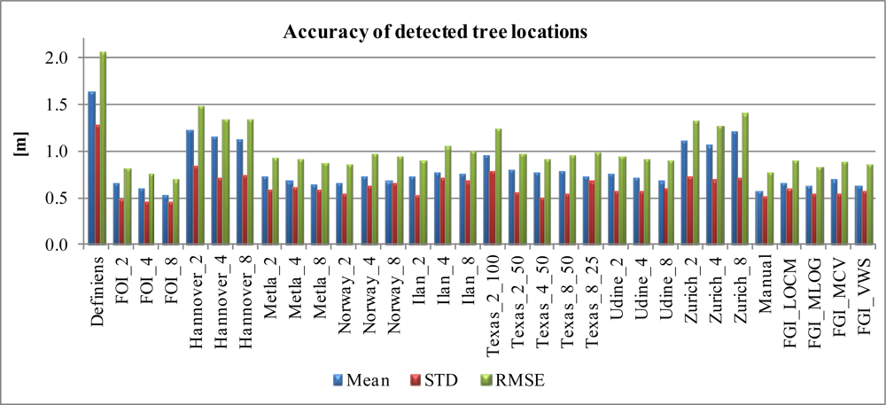
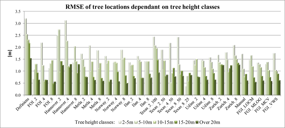
4.2. Accuracy of Determining Tree Location

The results on accuracy of tree location (Figure 7) clearly showed that the sensitivity of tree location is low as a function of point density and it mainly changes as a function of the model provider. Obviously, the calibration of the models has not been successful and several models overestimated the crown size (e.g., Definiens, Hannover, and Zürich). The detected tree positions of the best models show a standard deviation of less than 1m compared to the reference positions. For these models, the point density has a negligible effect on the resulting tree positions. For trees higher than 15 m, a standard deviation of 0.5 m was obtained for the tree positions. The automated models were as good as the manual processing of the point cloud in determining tree locations. Due to the method used for the evaluation of tree location, the capability errors in tree finding are included in the results, and therefore location accuracy as a function of tree height is of interest. FOI methods appear to be suitable for locating trees, but the results give an optimistic view of them since they found mainly the “more easily confirmable cases”, i.e., taller and isolated trees.

The results for the accuracy of tree location by tree height are shown in Figure 8. In general, as was to be expected, the taller a tree is, the better is the accuracy of location. It should be emphasized that the number of trees in the smaller tree classes was very low (on an average only 7.5 trees in height class 2–5 m), and the accuracy values should be carefully considered.

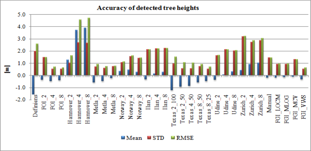
4.3. Accuracy of Tree Height

The investigated accuracy of the detected tree heights shows that different point densities have a negligible effect compared to the variability between the methods (Figure 9). The best models show a RMSE of 60 cm to 80 cm for the obtained tree heights. The methods of FOI, Metla, Texas, and FGI_VWS show the best accuracies. The results with the best automated models were significantly better than those attained when using the manual process. In general, underestimation of both tree height and standard deviation decreased as the point density increased. The overestimation produced by the Model Norway in regard to tree height was due to the correction applied to the tree height in the preprocessing phase. The methods capable of finding more trees in the lower classes obviously suffer; the uncertainty regarding the heights of the extracted tree in the lower levels is greater.

When the results for tree height accuracy as a function of tree height were computed, only trees with height difference between the reference and the model below 3 m were used (based on the results reported by Kaartinen and Hyyppä [27]). In the Hannover model, the errors were so large with bigger trees that trees belonging to height classes 15–20 m and over 20 m were omitted from the analysis. Figure 10 shows the results after the 3m filtering and deleting of outliers. In general, tree height did not appear to impact the accuracy of height determination, although the methods that are most feasible for smaller tree detection suffer the most. Surprisingly, the methods utilizing LM finding are among the best extraction techniques in regard to tree height accuracy.

4.4. Crown Delineation Accuracy

The results for total crown area appear to vary significantly between the models (Figure 11). The errors leading to false total crown area are as follows: inadequate tree finding capability (small trees missed), inadequate filtering of the raw point cloud data or DSM (leading to excessively large crowns, underestimating the number of trees), and inadequate calibration of the method using the given training data. With methods that represent the tree crown using a simple form such as a circle, it is possible that when the point density increases, the tree crown area also increases, as there are more hits on the outer branches of the trees. As the reference delineation is far more detailed than a circle, a circle often overestimates the area although a circle fitted to a crown which was modeled using a higher point density corresponds better to the outer branches. This can be seen, for example, in the Udine model’s results. The models tested more in practical forestry in boreal forest have already accumulated more experience in this calibration, i.e., FGI, FOI, and Norway methods.

5. Conclusions

The results confirmed that the extraction method is the main factor impacting achieved accuracy, as proposed by Kaartinen and Hyyppä [27], and that laser point density has less impact on individual tree detection.

Depending on the application, the criteria for tree detection and extraction can be different. For example, the methods that are most suitable for dominant tree detection should be used in flight obstacle mapping, power line monitoring, and telecommunication planning. In this evaluation, the best methods for dominant tree detection were FGI_MCV, FGI_LOCM, Norway, and Metla, and FOI if the pulse density is close to 8 points per m². They were also better than manual processing. For forest inventory, the method should be such that it is suitable of recording accurately the stand DBH distribution. Since DBHs are calculated for each individual tree based on height, tree species and crown size, the foremost criterion is correct height distribution. Allometric models describing the relationships between tree crown size, height, and DBH are highly sensitive to errors in the input data. Automated measurement results of tree crown size, in particular, tend to be prone to errors. Thus, the estimation of DBH on the basis of tree height and crown size results in a fairly significant degree of uncertainty. Nearest-neighbor methods applicable to single-tree interpretation are, therefore, currently under development [23,50,51]. The extracted data, acquired from detected trees, need to be calibrated with the ground truth, but it is vital that the method reveals as correctly as possible the number of dominant and suppressed trees with a small number of commission errors. This is an aspect where significant work has yet to be undertaken. Extracted individual trees can also be used in a simple way for improving area-based estimates with significantly improved accuracy and without using any calibrations [52], and thus individual tree extraction techniques are currently also important from the practical forestry point of view.

Based on the results of the present experiment, an approach using the high detection rate of FGI_MCV for all tree sizes (but further processing the suppressed tree data at the point level, as is done in the Zürich approach) is a solution deserving of more attention. Full waveform technology is also expected to improve individual tree detection, especially in the case of suppressed trees, as waveform analysis can be used to produce denser point clouds within the crowns. Additionally, a simple method based on LM finding (proposed, e.g., in Hyyppä et al. [20]) has turned out to be one of the best techniques applied in this experiment, and thanks to its simple implementation, it is especially feasible for commercial production.

In the tree cluster approach (TCA), the first phase is to segment CHM, as is done in many ITD approaches. In the second phase, accurately located field trees are linked to the corresponding segments [53–56]. Contrary to the ITD model, it is not assumed that a single segment represents a single tree. In the TCA, all the field trees located within the segments’ area are linked to corresponding segments. Thus, segments may include none, one, two or even more trees. This solves the tree detection problem in practice and the bias of the estimated area-level volume and basal-area is reduced.

Individual tree extraction is perhaps one of the few applications where automation provides higher quality than does manual processing. Vastaranta et al. [43] tried to improve the automatically detected trees with manual processing when acquiring reference for area-based inventory, but the accuracy of area-based predictions could not be improved. Several of the methods in the present experiment were superior to manual processing in dealing with dominant, co-dominant, and suppressed tree storeys. This also means that manually processed tree maps based on airborne laser surveys cannot be used as reference for developing automatic algorithms for tree detection, although this has been done previously. Inventories based on individual trees require reference data of individual trees collected in the field by some other means. Calibration is needed to reduce the underestimation of tree height and calibration of the basal area and stem volume (e.g., [57]).

In general, and as was to be expected, the taller a tree is, the better location accuracy is, as could be expected. Tree height accuracy, after high outliers had been deleted, was better than 0.5 m in all tree height classes when using the leading methods in this experiment, and this is a significant result, even though the number of the lowest level trees was small.

Solutions based on individual trees can be applied even with point densities of 2 points per m² or lower (e.g., [57]), but the optimum point density is most probably dependent on tree size and stand density of the forest. When dealing with sapling stands, a point density of 10 points per m² or higher is expected to increase the accuracy of the extraction results.

This international benchmarking experiment also demonstrated that the quality of one method versus other methods cannot be verified without testing the methods in the same forest conditions, since the effect of variability of forest conditions is believed to have a high impact on the achieved accuracy. This is evident when the results achieved in this study are compared to those reported in existing literature.

References

- Solodukhin, V.I.; Zukov, A.J.; Mazugin, I.N. Laser aerial profiling of a forest. Lew. NIILKh. Leningrad. Lesnoe Khozyaistvo 1977, 10, 53–58. (in Russian). [Google Scholar]
- Nelson, R.; Krabill, W.; Maclean, G. Determining forest canopy characteristics using airborne laser data. Remote Sens. Environ 1984, 15, 201–212. [Google Scholar]
- Schreier, H.; Lougheed, J.; Tucker, C.; Leckie, D. Automated measurements of terrain reflection and height variations using airborne infrared laser system. Int. J. Remote Sens 1985, 6, 101–113. [Google Scholar]
- Nelson, R.; Krabill, W.; Tonelli, J. Estimating forest biomass and volume using airborne laser data. Remote Sens. Environ 1988, 24, 247–267. [Google Scholar]
- Maclean, G.A.; Krabill, W.B. Gross-merchantable timber volume estimation using an airborne lidar system. Can. J. Remote Sens 1986, 12, 7–18. [Google Scholar]
- Currie, D.; Shaw, V.; Bercha, F. Integration of Laser Rangefinder and Multispectral Video Data for Forest Measurements. Proceedings of IGARSS’89, Vancouver, BC, Canada, 10–14 July 1989; 4, pp. 2382–2384.
- Bernard, R.; Vidal-Madjar, D.; Baudin, F.; Laurent, G. Nadir looking airborne radar and possible applications to forestry. IEEE Trans. Geosci. Remote Sens 1987, 21, 297–309. [Google Scholar]
- Hallikainen, M.; Hyyppä, J.; Somersalo, E. Classification of Forest Types by Microwave Remote Sensing. Proceedings of EARSeL 9th General Assembly and Symposium, Espoo, Finland, 27 June–1 July 1989; pp. 293–298.
- Hyyppä, J.; Hallikainen, M.; Pulliainen, J. Accuracy of Forest Inventory Based on Radar-Derived Stand Profile. Proceedings of IGARSS’93, Tokyo, Japan, 18–21 August 1993; pp. 391–393.
- Hyyppä, J.; Hallikainen, M.; Hyyppä, H. A Scanning Ranging Radar for Forest Inventory. Proceedings of URSI/IEEE/IRC XXI National Convention on Radio Science 1996, Espoo, Finland, 2–3 October 1996; Report S 222. pp. 255–256.
- Hyyppä, J.; Hyyppä, H.; Inkinen, M. Capabilities of Multi-Source Remote Sensing for Forest Inventory. Proceedings of 3rd International Airborne Remote Sensing Conference and Exhibition, Copenhagen, Denmark, 7–10 July 1997.
- Kraus, K.; Pfeifer, N. Determination of terrain models in wooded areas with airborne laser scanner data. ISPRS J. Photogramm 1998, 53, 193–203. [Google Scholar]
- Vosselman, G. Slope Based Filtering of Laser Altimetry Data. Proceedings of XIXth ISPRS Congress Technical Commission III: Systems for Data Processing, Analysis and Representation, Amsterdam, The Netherlands, 16–23 July 2000. In International Archives of the Photogrammetry, Remote Sensing and Spatial Information Sciences; ISPRS: Vienna, Austria, 2000; Volume 33, No. B3/2, pp. 935–942..
- Næsset, E. Determination of mean tree height of forest stands using airborne laser scanner data. ISPRS J. Photogramm 1997, 52, 49–56. [Google Scholar]
- Næsset, E. Estimating timber volume of forest stands using airborne laser scanner data. Remote Sens. Environ 1997, 61, 246–253. [Google Scholar]
- Hyyppä, H.; Hyyppä, J. Comparing the accuracy of laser scanner with other optical remote sensing data sources for stand attributes retrieval. Photogramm. J. Fin 1999, 16, 5–15. [Google Scholar]
- Hyyppä, J.; Inkinen, M. Detecting and estimating attributes for single trees using laser scanner. Photogramm. J. Fin 1999, 16, 27–42. [Google Scholar]
- Brandtberg, T. Automatic Individual Tree-Based Analysis of High Spatial Resolution Remotely Sensed Data. Ph.D. Thesis, Acta Universitatis Agriculturae Sueciae, Silvestria 118, Swedish University of Agricultural Sciences, Uppsala, Sweden, 1999.
- Ziegler, M.; Konrad, H.; Hofrichter, J.; Wimmer, A.; Ruppert, G.; Schardt, M.; Hyyppä, J. Assessment of forest attributes and single-tree segmentation by means of laser scanning. Proc. SPIE 2000, 4035, 73–84. [Google Scholar]
- Hyyppä, J.; Schardt, M.; Haggrén, H.; Koch, B.; Lohr, U.; Scherrer, H.U.; Paananen, R.; Luukkonen, H.; Ziegler, M.; Hyyppä, H.; et al. HIGH-SCAN: The first European-wide attempt to derive single-tree information from laserscanner data. Photogramm. J. Fin 2001, 17, 58–68. [Google Scholar]
- Brandtberg, T.; Warner, T.; Landenberger, R.; McGraw, J. Detection and analysis of individual leaf-off tree crowns in small footprint, high sampling density lidar data from the eastern deciduous forest in North America. Remote Sens. Environ 2003, 85, 290–303. [Google Scholar]
- Holmgren, J.; Persson, Å. Identifying species of individual trees using airborne laser scanning. Remote Sens. Environ 2004, 90, 415–423. [Google Scholar]
- Yu, X.; Hyyppä, J.; Kaartinen, H.; Maltamo, M. Automatic detection of harvested trees and determination of forest growth using airborne laser scanning. Remote Sens. Environ 2004, 90, 451–462. [Google Scholar]
- Næsset, E. Predicting forest stand characteristics with airborne scanning laser using a practical two-stage procedure and field data. Remote Sens. Environ 2002, 80, 88–99. [Google Scholar]
- Holopainen, M.; Vastaranta, M.; Rasinmäki, J.; Kalliovirta, J.; Mäkinen, A.; Haapanen, R.; Melkas, T.; Yu, X.; Hyyppä, J. Uncertainty in timber assortment estimates predicted from forest inventory data. Eur. J. For. Res 2010, 129, 1131–1142. [Google Scholar]
- Falkowski, M.; Smith, A.; Gessler, P.; Hudak, A.; Vierling, L.; Evans, J. The influence of the conifer forest canopy cover on the accuracy of two individual tree detection algorithms using lidar data. Can. J. Remote Sens 2008, 34, 1–13. [Google Scholar]
- Kaartinen, H.; Hyyppä, J. EuroSDR/ISPRS Project, Commission II “Tree Extraction”; Final Report; Official Publication no 53; EuroSDR (European Spatial Data Research): Dublin, Ireland, 2008. [Google Scholar]
- Vastaranta, M.; Holopainen, M.; Yu, X.; Hyyppä, J.; Mäkinen, A.; Rasinmäki, J.; Melkas, T.; Kaartinen, H.; Hyyppä, H. Effects of ALS individual tree detection error sources on forest management planning calculations. Remote Sens 2011, 3, 1614–1626. [Google Scholar]
- Holopainen, M.; Mäkinen, A.; Rasinmäki, J.; Hyyppä, J.; Hyyppä, H.; Kaartinen, H.; Viitala, R.; Vastaranta, M.; Kangas, A. Effect of tree level airborne laser scanning accuracy on the timing and expected value of harvest decisions. Eur. J. For. Res 2010, 29, 899–910. [Google Scholar]
- Persson, Å.; Holmgren, J.; Söderman, U. Detecting and measuring individual trees using an airborne laser scanner. Photogramm. Eng. Remote Sensing 2002, 68, 925–932. [Google Scholar]
- Leckie, D.; Gougeon, F.; Hill, D.; Quinn, R.; Armstrong, L.; Shreenan, R. Combined high-density lidar and multispectral imagery for individual tree crown analysis. Can. J. Remote Sens 2003, 29, 633–649. [Google Scholar]
- Straub, B. A Top-Down Operator for the Automatic Extraction of Trees: Concept and Performance Evaluation. Proceedings of the ISPRS Working Group III/3 Workshop ‘3-D Reconstruction from Airborne Laserscanner and InSAR Data’, Dresden, Germany, 8–10 October 2003; pp. 34–39.
- Popescu, S.; Wynne, R.; Nelson, R. Measuring individual tree crown diameter with lidar and assessing its influence on estimating forest volume and biomass. Can. J. Remote Sens 2003, 29, 564–577. [Google Scholar]
- Andersen, H-E.; Reutebuch, S.; Schreuder, G. Bayesian Object Recognition for the Analysis of Complex Forest Scenes in Airborne Laser Scanner Data. Proceedings of ISPRS Commission III, Symposium 2002 Photogrammetric Computer Vision, Graz, Austria, 9–13 September 2002. In International Archives of the Photogrammetry, Remote Sensing and Spatial Information Sciences; ISPRS: Vienna, Austria, 2002; Volume 34, part 3A, pp. 35–41..
- Morsdorf, F.; Meier, E.; Kötz, B.; Itten, K. I.; Dobbertin, M.; Allgöwer, B. LIDAR-based geometric reconstruction of boreal type forest stands at single tree level for forest and wildland fire management. Remote Sens. Environ 2004, 3, 353–362. [Google Scholar]
- Wack, R.; Schardt, M.; Lohr, U.; Barrucho, L.; Oliveira, T. Forest Inventory for Eucalyptus Plantations Based on Airborne Laser Scanner Data. Proceedings of ISPRS Workshop 3-D Reconstruction from Airborne Laserscanner and InSAR Data, Dresden, Germany, 8–10 October 2003. In International Archives of the Photogrammetry, Remote Sensing and Spatial Information Sciences; ISPRS: Vienna, Austria, 2003; Volume 34, Part 3/W13, pp. 40–46.
- Pitkänen, J.; Maltamo, M.; Hyyppä, J.; Yu, X. Adaptive Methods for Individual Tree Detection on Airborne Laser Based Canopy Height Model. Proceedings of ISPRS Workshop Laser-Scanners for Forest and Landscape Assessment, Freiburg, Germany, 3–6 October 2004. In International Archives of Photogrammetry, Remote Sensing and Spatial Information Sciences; ISPRS: Vienna, Austria, 2004; Volume 36, Part 8/W2, pp. 187–191..
- Yu, X.; Hyyppä, J.; Vastaranta, M.; Holopainen, M.; Viitala, R. Predicting individual tree attributes from airborne laser point clouds based on random forests technique. ISPRS J. Photogramm 2011, 66, 28–37. [Google Scholar]
- Heinzel, J.N.; Weinacker, H.; Koch, B. Prior-knowledge-based single-tree extraction. Int. J. Remote Sens 2011, 32, 4999–5020. [Google Scholar]
- Vauhkonen, J.; Ene, L.; Gupta, S.; Heinzel, J.; Holmgren, J.; Pitkänen, J.; Solberg, S.; Wang, Y.; Weinacker, H.; Hauglin, K.M.; et al. Comparative testing of single-tree detection algorithms under different types of forest. Forestry 2011. [Google Scholar] [CrossRef]
- Peuhkurinen, J.; Maltamo, M.; Malinen, J.; Pitkänen, J.; Packalén, P. Preharvest measurement of marked stands using airborne laser scanning. Forest Sci 2007, 53, 653–661. [Google Scholar]
- Falkowski, M.J.; Smith, A.M.S.; Gessler, P.E.; Hudak, A.T.; Vierling, L.A.; Evans, J.S. The influence of conifer forest canopy cover on the accuracy of two individual tree measurement algorithms using lidar data. Can. J. Remote Sens 2008, 34, 338–350. [Google Scholar]
- Vastaranta, M.; Kankare, V.; Holopainen, M.; Yu, X.; Hyyppä, J.; Hyyppä, H. Combination of individual tree detection and area-based approach in imputation of forest variables using airborne laser data. ISPRS J. Photogramm 2012, 67, 73–79. [Google Scholar]
- Axelsson, P. Ground Estimation of Laser Data Using Adaptive TIN Models. Proceedings of OEEPE Workshop on Airborne Laserscanning and Interferometric SAR for Detailed Digital Elevation Models, Stockholm, Sweden, 1–3 March 2001; Publication No. 40. pp. 185–208.
- Bilker, M.; Kaartinen, H. The Quality of Real-Time Kinematic (RTK) GPS Positioning; Reports of the Finnish Geodetic Institute; FGI: Masala, Finland, 2001; pp. 1–25. [Google Scholar]
- Wolf (né Straub), B.-M.; Heipke, C. Automatic extraction and delineation of single trees from remote sensing data. Machine Vis. Appl 2007, 18, 317–330. [Google Scholar]
- Solberg, S.; Næsset, E.; Bollandsås, O.M. Single-tree segmentation using airborne laser scanner data in a structurally heterogeneous spruce forest. Photogramm. Eng. Rem. Sensing 2006, 72, 1369–1378. [Google Scholar]
- Serra, J. Image Analysis and Mathematical Morphology; Academic Press: London, UK, 1982; Volume 1. [Google Scholar]
- Serra, J. Image Analysis and Mathematical Morphology: Theoretical Advances; Academic Press: London, UK, 1988; Volume 2. [Google Scholar]
- Maltamo, M.; Peuhkurinen, J.; Malinen, J.; Vauhkonen, J.; Packalén, P.; Tokola, T. Predicting tree attributes and quality characteristics of Scots pine using airborne laser scanning data. Silva Fennica 2009, 43, 507–521. [Google Scholar]
- Vauhkonen, J.; Korpela, I.; Maltamo, M.; Tokola, T. Imputation of single-tree attributes using airborne laser scanning-based height, intensity, and alpha shape metrics. Remote Sens. Environ 2010, 114, 1263–1276. [Google Scholar]
- Hyyppä, J.; Yu, X.; Hyyppä, H.; Vastaranta, M.; Holopainen, M.; Kukko, A.; Kaartinen, H.; Jaakkola, A.; Vaaja, M.; Koskinen, J.; Alho, A. Improved forest inventory using penetrated Hits and data fusion at feature level. Remote Sens 2012. submitted. [Google Scholar]
- Hyyppä, J.; Mielonen, T.; Hyyppä, H.; Maltamo, M.; Honkavaara, E.; Yu, X.; Kaartinen, H. Using Individual Tree Crown Approach for Forest Volume Extraction with Aerial Images and Laser Point Clouds. Proceedings of The ISPRS Workshop Laser Scanning 2005, Enschede, The Netherlands, 12–14 September 2005. In International Archives of Photogrammetry, Remote Sensing and Spatial Information Sciences, ISPRS: Vienna, Austria, 2005; Volume 36, Part 3/W19, pp. 144–149..
- Hyyppä, J.; Yu, X.; Hyyppä, H.; Maltamo, M. Methods of Airborne Laser Scanning for Forest Information Extraction. Presented at Workshop on 3D Remote Sensing in Forestry, Vienna, Austria, 14–15 February 2006; CD-ROM. p. 16.
- Lindberg, E.; Holmgren, J.; Olofsson, K.; Wallerman, J.; Olsson, H. Estimation of tree lists from airborne laser scanning by combining single-tree and area-based methods. Int. J. Remote Sens 2010, 31, 1175–1192. [Google Scholar]
- Breidenbach, J.; Næsset, E.; Lien, V.; Gobakken, T.; Solberg, S. Prediction of species specific forest inventory attributes using a nonparametric semi-individual tree crown approach based on fused airborne laser scanning and multispectral data. Remote Sens. Environ 2010, 114, 911–924. [Google Scholar]
- Vastaranta, M.; Holopainen, M.; Yu, X.; Haapanen, R.; Melkas, T.; Hyyppä, J.; Hyyppä, H. Individual tree detection and area-based approach in retrieval of forest inventory characteristics from low-pulse airborne laser scanning data. Photogramm. J. Fin 2011, 22, 1–13. [Google Scholar]