Article

Utility of Satellite and Aerial Images for Quantification of Canopy Cover and Infilling Rates of the Invasive Woody Species Honey Mesquite (Prosopis Glandulosa) on Rangeland

Texas AgriLife Research, P.O. Box 1658, 11708 Hwy 70 South, Vernon, TX 76385, USA
*
Author to whom correspondence should be addressed.
Remote Sens. 2012, 4(7), 1947-1962; https://0-doi-org.brum.beds.ac.uk/10.3390/rs4071947
Submission received: 9 May 2012 / Revised: 5 June 2012 / Accepted: 25 June 2012 / Published: 29 June 2012

Abstract

:
Woody plant encroachment into grasslands and rangelands is a world-wide phenomenon but detailed descriptions of changes in geographical distribution and infilling rates have not been well documented at large land scales. Remote sensing with either aerial or satellite images may provide a rapid means for accomplishing this task. Our objective was to compare the accuracy and utility of two types of images with contrasting spatial resolutions (1-m aerial and 30-m satellite) for classifying woody and herbaceous canopy cover and determining woody infilling rates in a large area of rangeland (800 km2) in north Texas that has been invaded by honey mesquite (Prosopis glandulosa). Accuracy assessment revealed that the overall accuracies for the classification of four land cover types (mesquite, grass, bare ground and other) were 94 and 87% with kappa coefficients of 0.89 and 0.77 for the 1-m and 30-m images, respectively. Over the entire area, the 30-m image over-estimated mesquite canopy cover by 9 percentage units (10 vs. 19%) and underestimated grass canopy cover by the same amount when compared to the 1-m image. The 30-m resolution image typically overestimated mesquite canopy cover within 225 4-ha sub-cells that contained a range of mesquite covers (1–70%) when compared to the 1-m image classification and was not suitable for quantifying infilling rates of this native invasive species. Documenting woody and non-woody canopy cover on large land areas is important for developing integrated, regional-scale management strategies for rangeland and grassland regions that have been invaded by woody plants.

Graphical Abstract

1. Introduction

Woody plant encroachment on non-agricultural lands (e.g., grasslands and rangelands) is a world-wide phenomenon [14]. Causes are attributed to a variety of factors including fire suppression, accelerated seed distribution via livestock consumption and fecal deposition, reduced competition from grasses due to livestock overgrazing, and increased atmospheric CO2 concentrations that favor growth of C3 woody species over C4 grasses [1,57].
In the southern Great Plains and southwestern United States, a native legume, honey mesquite (Prosopis glandulosa), has invaded a significant amount of grasslands and rangelands [1,8,9]. High densities of mesquite can negatively affect these lands by reducing grass growth and livestock production [7,10,11], altering nutrient and hydrologic cycling [12,13] and increasing potential for soil erosion [9]. In contrast, the presence of mesquite either in savannas or dense woodlands may be beneficial for wildlife habitat and herbaceous diversity [14,15]. In addition, woodland thickets may have utility for ecosystem carbon storage and bioenergy uses [1618]. Because these potentially detrimental and beneficial effects often become significant only at large spatial scales (e.g., impacting livestock grazing, watershed function, wildlife habitat) and at certain density and canopy cover levels [10,11], accurate and detailed mapping of woody distribution at such scales is essential for determining extant conditions and invasion rates and developing long-term management plans for these regions.
Although the general distribution of mesquite species has been described in many regions of the world [1922], there is little detailed information concerning geographical distribution of canopy cover at large (e.g., >100 km2) scales [2325]. Also, there has been little documentation at such scales of changes in woody distribution patterns that might include developments of new invasion fronts or infilling rates within areas already occupied.
Quantifying woody and grass cover at large geographic scales is difficult with ground surveys because of the time and labor required and no access to many areas [2,26,27]. Therefore, remote sensing has received considerable attention as a rapid and inexpensive method for quantifying vegetation distribution on large land areas [28,29]. A wide range of sensor systems including aerial photographs, airborne and satellite multispectral and hyperspectral sensors have been employed for separately mapping rangeland woody and grass components [2,30,31]. Successful separation of these components is usually linked to differences in reflectance properties because of phenological differences at the time the image was obtained [2,27,32,33]. For example, several studies have shown that mesquite canopy cover in Texas can be distinguished from grassland vegetation in late-summer and fall when mesquite is in full foliage and the bulk of the grass community is dormant [1,10,2325,33].
A typical and inexpensive method for mapping woody cover on large land areas is to employ satellite imagery such as Landsat 5 Thematic Mapper (TM). However, the 30-m resolution of these images may not be adequate for detecting subtle changes in distribution patterns and infilling rates. The recent availability of National Agricultural Imagery Program (NAIP) images provides an inexpensive source of images covering extensive land areas (data sets are at the county level) at a much higher resolution (1 and 2-m) [25,34]. This provided us with the opportunity to contrast the accuracy of these two image sources with respect to mapping mesquite at a large geographic scale and detecting changes in infilling rates within currently invaded regions. Our objectives were: (1) to compare absolute values and classification accuracy of mesquite, dormant grasses and bare ground using images with two spatial resolutions (1-m and 30-m); and (2) to compare the utility of 1-m and 30-m image types for detecting different percent covers on small 1-km2 patches as an indication of infilling rates.

2. Materials and Methods
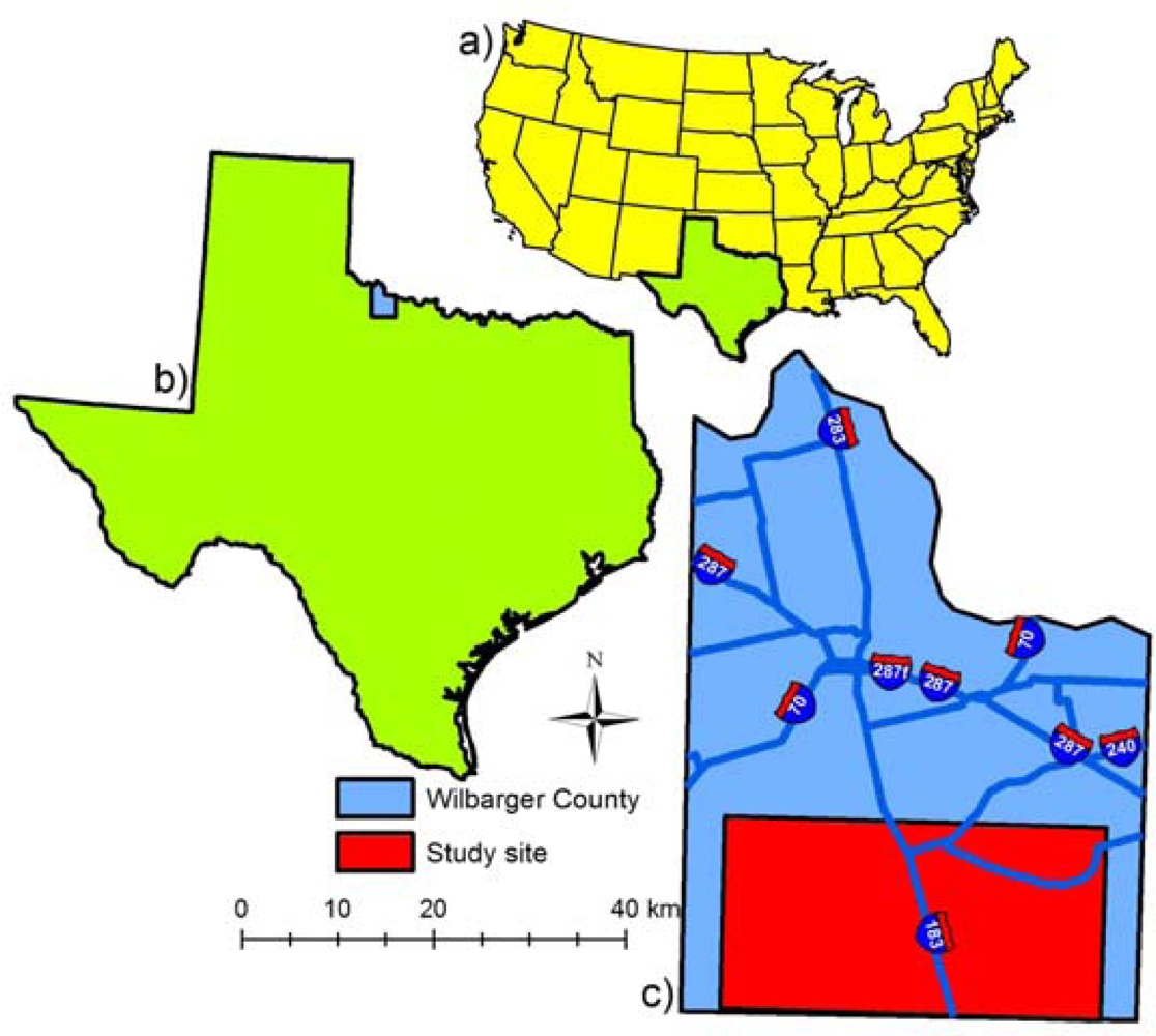
2.1. Study Region

The research was conducted on an 800 km2 (20 km by 40 km; 80,000 ha) area consisting of mainly mesquite/grass rangeland located on the southern part of Wilbarger County located on the northeastern Rolling Plains Ecological Region of Texas (Figure 1). Mean annual precipitation is 660 mm, bi-modally distributed with peak months in May and September. Woody overstory vegetation on the rangeland areas consists primarily of mesquite at 1–80% cover. Rangeland herbaceous species consist of a mixture of C3 and C4 grasses, including Texas wintergrass (Nassella leucotricha), little bluestem (Schizachyrium scoparium), blue grama (Bouteloua gracilis), sideoats grama (Bouteloua curtipendula), Indiangrass (Sorghastrum nutans), and sand bluestem (Andropogon hallii). Other species found in smaller amounts (<1%) are lotebush (Ziziphus obtusifolia var. obrusifolia), tasajillo (Opuntia leptocaulis), and tulip pricklypear (Opuntia polyacantha) [911]. Cottonwood (Populus deltoides), American elm (Ulmus Americana), hackberry (Celtis occidentalis), western soapberry (Sapindus saponaria), and saltcedar (Tamarix ramosissima) trees occur along narrow riparian zones. Soils consist of a variety of series, most with a loam or clay loam texture [9,15,23,24].

2.2. Image Acquisition

Images used for classification were (1) a four-band aerial composite image of Wilbarger County, TX obtained from the National Agricultural Imagery Program (NAIP), Natural Resources Conservation Service (NRCS) Geospatial Data Gateway ( http://datagateway.nrcs.usda.gov) with a spatial resolution of 1 m by 1 m (hereafter 1-m image), and (2) a seven-band Landsat 5 Thematic Mapper (TM) level 1 product as GEOTIFF image files obtained from the United States Geological Survey (USGS; http://glovis.usgs.gov) with a spatial resolution of 30 m by 30 m (hereafter 30-m image).
The 1-m image consisted of a composite of aerial images obtained by the NRCS during 26–27 September 2008, and the 30-m image was acquired by the USGS on 2 October 2008. For both time periods, mesquite and other woody canopies were in full foliage and the grassland understory was dormant, providing a strong color contrast between woody canopies, grass areas and bare ground. The 1-m NAIP image was projected to the Universal Transverse Mercator North American Datum 1983 Zone 14 North, and the 30-m image was projected to the Universal Transverse Mercator World Geodetic System 1984 Zone 14 North by the providers. The 30-m image projection was converted to the Universal Transverse Mercator North American Datum 1983 Zone 14 North using image warping in Environment for Visualizing Images (ENVI) software (Exelis Visual Information Solutions, Boulder, CO, USA). The 1-m image NAIP database was compiled at the county level, whereas the 30-m image extended over multiple counties in north Texas. Image to image warping using easily identifiable landmarks such as road corners and intersections, buildings, and water tanks in both the 1-m and 30-m images resulted in accurate alignment of the two images Atmospheric correction was not applied to the 30-m image because in many applications involving classification and change detection, atmospheric correction is unnecessary as long as the imagery to be classified and the training data are in the same relative scale [35]. The 1-m image NAIP database was compiled at the county level, whereas the 30-m image extended over multiple counties in north Texas.

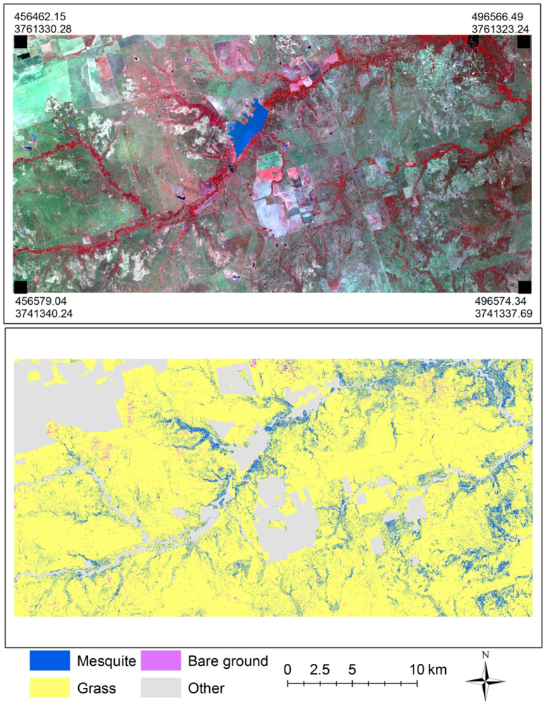
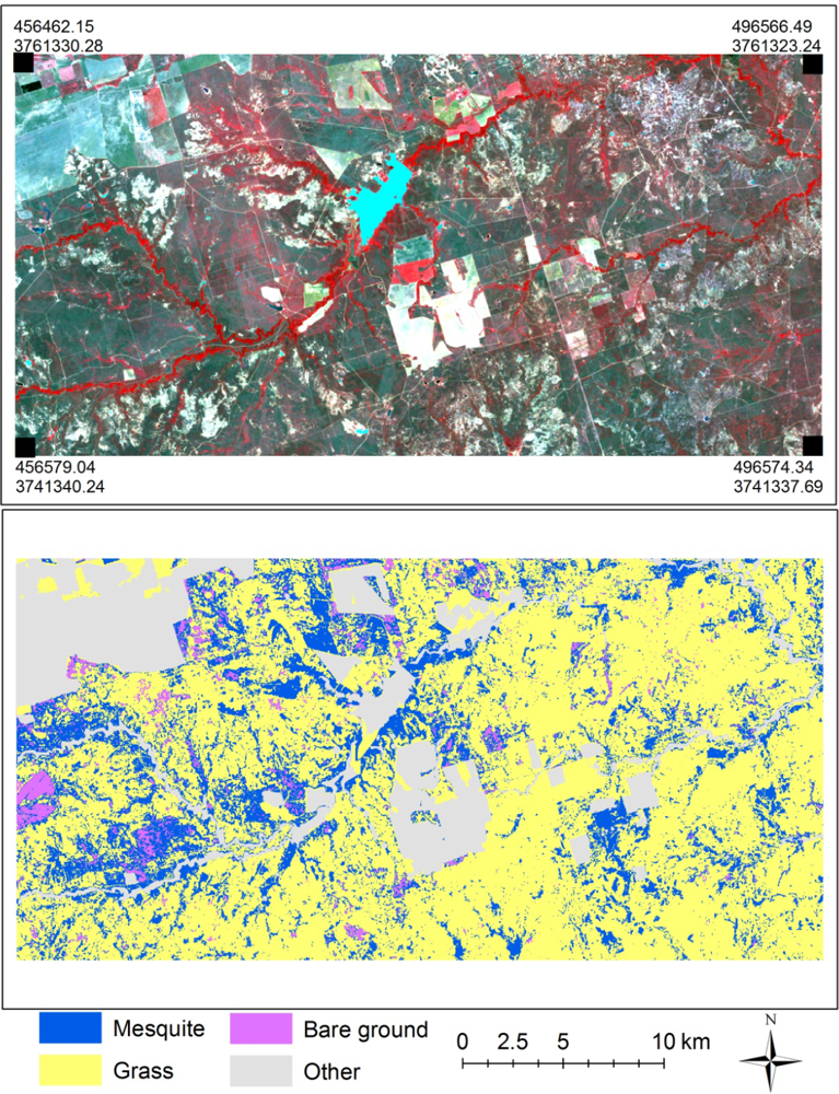
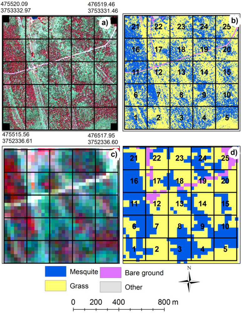
2.3. Objective 1: Image Classification and Accuracy Assessment

To address Objective 1, the following land cover types were classified for both images: mesquite cover, grass cover, bare ground and “other.” The “other” class was comprised all land cover types that were not included in the first three types and included residential areas, roads, water bodies, fallow and actively growing cropland, and non-mesquite woody plants in narrow riparian areas (Figures 2 and 3).
Classification of cover types was conducted using the Feature Analyst (Visual Learning Systems, Missoula, MT, USA) in the ArcGIS (ESRI Inc. Redland, CA, USA) software program. The Feature Analyst is an object-based segmentation and classification method, which has been designed as a plug-in toolset for use with established GIS and remote sensing software such as ArcGIS, ERDAS Imagine, SOCET SET, GeoMedia, and RemoteView [34,36,37]. The Feature Analyst provides a suite of inductive learning algorithms for object recognition using both spectral and spatial characteristics and includes a feature extraction function that identifies object-specific features defined by a user. The software uses spatial context when extracting features and provides a natural, hierarchical learning approach including variants of artificial neural networks, decision trees, Bayesian, K-nearest neighbor, and ensemble learning. Land cover training classes used in Feature Analyst were created by manually digitizing 50 polygons of each land cover type at identified locations on the images and on the ground. Each polygon consisted of 100–300 pixels in the 1-m image and 5–10 pixels in the 30-m image. The first four bands (1, 2, 3, 4) of the 30-m image and all bands of the 1-m image were used for classification.
For the accuracy assessment, 500 ground verification (i.e., “ground-truthing”) points were randomly generated on the images using the “create random points” function in ArcGIS. The verification points were then identified on the ground after loading the geospatial coordinates of each point into a real time differential Trimble GeoXH Global Positioning System (Trimble Navigation Limited, Sunnyvale, CA, USA) equipped with ArcPad (ESRI Inc. Redland, CA, USA) software that provided sub-meter (10-cm) accuracy. Of the 500 verification points, 135 points were found to be inaccessible, and the remaining 365 locations were used for accuracy assessment. At each ground-truthing location, land cover classes within a 1-m radius for the 1-m image and within a 30-m radius for the 30-m image were visually assessed on the ground and recorded. Each ground-level land cover class was then compared with image classification results for accuracy assessment. The same set of ground-truthing locations was used for both the 1 and 30-m image classifications. Accuracy assessment for the land cover classifications was made by constructing an error matrix for each image, which compared, on a group by group basis, the relationship between known actual (reference) categories as verified on the ground and corresponding classified categories. The overall, user’s and producer’s accuracies were calculated from the error matrix. In addition to accuracy, the kappa coefficient was calculated from the error matrix [37,38].

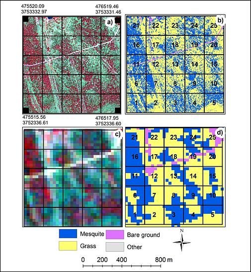
2.4. Objective 2: Infilling Detection

To address Objective 2, the total study area was divided into 800, 1 km by 1 km cells. From this we visually selected 9 cells that appeared to contain a variety of mesquite canopies with different densities. Each of these 9 cells was further subdivided into 25 sub-cells (each 200 m by 200 m, or 4 ha) for a total of 225 sub-cells (Figure 4). Percent land cover of the 4 cover types (mesquite, grass, bare, other) was determined for each sub-cell on both the 1-m and 30-m images. A scatter plot of percent mesquite cover for each sub-cell from the 1-m (x-axis) and 30-m (y-axis) images was developed and compared to a 1:1 line. The 1-m image mesquite cover values on the x-axis were then divided into seven groups: <5, 5–10, 10–20, 20–30, 30–40, 40–50, and 50–70% (there were no mesquite cover values from the 1-m image that exceeded 70%) and a simple tally of the number of points in the scatter plot that fell above or below the 1:1 line was then determined for each group. This provided an indication of whether the 30-m images were over- or under-estimating mesquite cover with the assumption that cover determined on the 1-m images was more accurate. The mean absolute deviation of all points within each of the seven cover groups was determined as a measure of the degree of deviation of cover generated from the 30-m image compared to the 1-m image.
Trend lines and regression equations were determined by using the SigmaPlot/SigmaStat 11.0 (Systat Software, Inc., San Jose, CA, USA) curve fitting feature in which a general equation is selected and the program determines the best fit curve and coefficients for that equation. A logarithmic curve (if x > 0; f = y0 + a × ln (x)) was fitted to Figure 5(b) and a quadratic curve (f = y0 + ax + bx2) was fitted to Figure 5(c). Mesquite cover categories on the x-axis were assigned whole number values of 1 through 6 in Figure 5(b,c) to determine the trend lines and r2 values.

3. Results

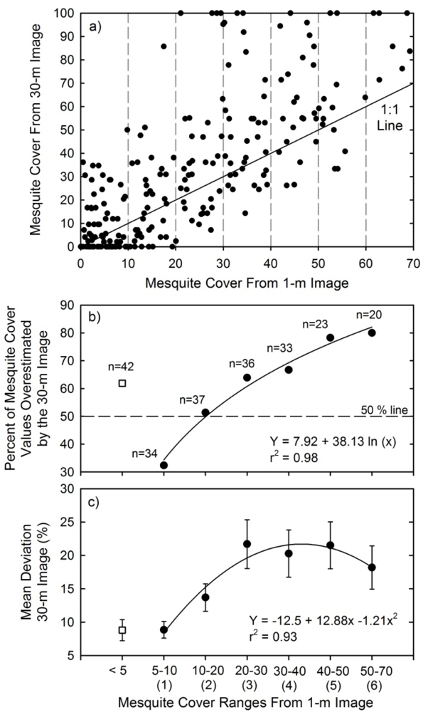
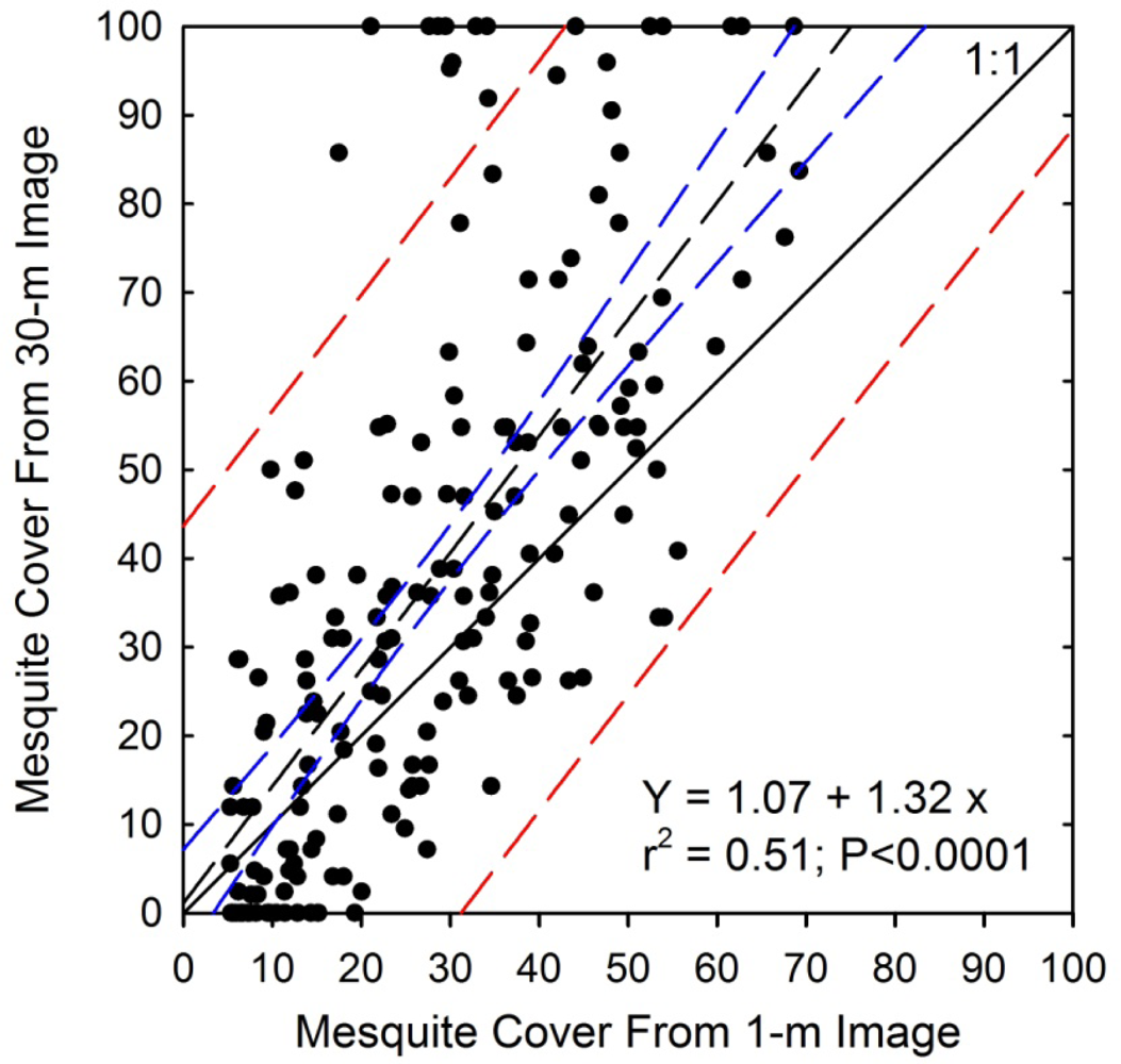
3.1. Objective 1: Classification and Accuracy of 1-m and 30-m Images

Overall classification of the 1-m image indicated that the 800 km2 study area was comprised of 10% (81 km2) mesquite, 75% (602 km2) grass, 1% (5 km2) bare ground, and 14% (114 km2) “other” land cover classes (Table 1). Mesquite cover was 9 percentage units greater in the 30-m image classification compared to the 1-m image. Grassland areas were 9 percentage units and 12% lower in the 30-m image compared to the 1-m image. Bare ground was <1% in both images but was 45% greater in the 30-m image compared to the 1-m image. There was little difference between images in percent cover of “other” land types. Both images delineated an equal amount of rangeland (i.e., mesquite + grass cover) from cropland and other land cover types.
Accuracy assessments indicated that the 1-m image yielded a higher overall accuracy compared to 30-m image. Overall, 94% of the known ground truth points were classified correctly on the 1-m image with a kappa value of 0.89 (Table 2). Producer’s accuracies were 94, 95, 100 and 89%, and user’s accuracies were 93, 97, 63 and 86% for mesquite, grass, bare ground and other classes, respectively. The overall accuracy for the 30-m image was 87% with a kappa value of 0.77. Producer’s accuracies were 90, 87, 100 and 80%, and user’s accuracies were 84, 96, 100, and 65% for mesquite, grass, bare ground, and other cover classes, respectively.

3.2. Objective 2: Infilling Detection in Sub-cells

The scatter plot of mesquite cover in the 1-m compared to 30-m resolution sub-cells indicated a great deal of variation and deviation from the 1:1 line (Figure 5(a)). With the 30-m data on the y-axis, most of the points were located above the 1:1 line and this trend appeared to increase with increasing overall cover. Mesquite cover in 18 sub-cells was classified as being >90% in the 30-m image, while no sub-cell had >70% cover in the 1-m image.
Within each of the seven established mesquite cover ranges, the percentage of sub-cells that yielded points above the 1:1 line increased in a tight curvilinear pattern (r2 = 0.98) from about 32% in the 5–10% mesquite cover range to 80% in the 50–70% cover range (Figure 5(b)). Any Y-axis value in Figure 5(b) that was <50% indicates that the 30-m image usually underestimated mesquite cover, while any value >50% indicates an overestimate (50% line shown). Thus, the 30-m image mostly underestimated mesquite cover at 5–10% actual mesquite cover, accurately estimated cover at 10–20% actual cover, and mostly overestimated cover at actual canopy covers >20%. The curvilinear function indicates that there was a trend of diminishing overestimation as cover increased (Figure 5(b)). The degree of deviation of the 30-m image estimates of mesquite cover from the 1-m image estimates (i.e., from the 1:1 line in Figure 5(a)) followed a curvilinear pattern and was at maximum in the mesquite cover ranges of 20–50% (Figure 5(c)).
The single exception to this pattern was when mesquite cover estimates from the 1-m image were <5%. In this range, over 60% of the sub-cells in the 30-m image overestimated mesquite cover (Figure 5(b)), and some of these mesquite cover values exceeded 30% (as seen in Figure 5(a)), even though the 1-m image determined cover to be <5%.
Figure 6 displays a scatter plot of the data from Figure 5(a) with the 42 points that fell within the <5% cover class (in Figure 5(b)) eliminated. The regression of these remaining 183 points revealed that the slope of the regression line increasingly deviated from the 1:1 line (Figure 6). The 95% CI was narrow and the significance of the regression was high due to the large number of points. However, any points that fell outside the 95% prediction band (red lines) were all on the upper side indicating an overestimate of cover values by the 30-m image.

4. Discussion

Although there is no set standard for classification accuracy, Foody et al. [39] recommended an accuracy target of 85% and Thomlinson et al. [40] set an overall accuracy target of 85% with no individual class accuracy less than 70%. Based on these accuracy recommendations, classification of the 1-m and 30-m images both met the overall and individual class accuracies with the exception of two classification categories: bare ground from the 1-m image and “other” from the 30-m image classification. Even though both images met a general classification accuracy level as defined in the literature, the overall classification accuracy was different between the images.
The higher overall classification accuracy of the 1-m image compared to 30-m image was expected because in cases where mesquite canopy or grass patch sizes were smaller than the 900 m2 image pixel size, they could not be reliably detected using the feature extraction methods in the 30-m image due to the patch being mixed within a pixel or among pixels. Indeed, a detailed-visual comparison between the 30-m classified image and the 1-m non-classified color infrared image, coupled with ground surveys, indicated that most of the misclassified pixels for a given cover type were composed of a mosaic of different materials and the smaller target within the pixel was dominated by a larger cover category.
Because the absolute cover values of bare ground and “other” were similar between the 1-m and 30-m images (see Table 1), the difference of 9 percentage units of mesquite cover and 9 percentage units of grass cover between these images was likely due to a direct replacement of grass cover with mesquite cover. If we assume the 1-m image yielded the more accurate value for mesquite cover, and our accuracy data appear to verify this, we can then assume that the 30-m image replaced about 9 percentage units of what was in reality grass cover with that of mesquite cover. Reasons for this are unclear but in some locations the 30-m pixels that were located on the margins of mesquite patches may have extended those margins beyond their true borders. In other locations, an isolated patch of mesquite that was <900 m2 but still of a reasonable size (e.g., 500–800 m2) may have been recorded in the 30-m image as a full 900 m2 pixel of mesquite cover, whereas, it would have been recorded more accurately by the 1-m image as being <900 m2 total area. We did not investigate the minimum threshold at which the smallest mesquite patch would still register as a full pixel of mesquite cover on a 30-m image. This would vary depending on where within the 30-m pixel the mesquite patch occurred.
From an applied management standpoint, differences in the estimate of mesquite cover between the 1-m and 30-m images, as shown in this study, could have important consequences regarding image interpretation and development of resource management plans. For example, mesquite at 10% cover—as determined for the entire study region by the 1-m image—does not negatively affect grass production significantly, but it could significantly reduce grass production at 19% cover, as determined by the 30-m image. If the 1-m cover value was slightly higher (e.g., 15–20%), then these comparisons would be much more dramatic as [11] has shown there is a rapid drop off in C4 mid-grass production when mesquite cover exceeds 25%. Therefore landscape scale management decisions could be significantly compromised if they were based solely on mesquite cover and grass production estimates from the 30-m images. Similar errors are possible when assessing other management variables, such as amount and extent of mesquite cover for wildlife habitat, amount of open grassland for grassland bird habitat, or woody based carbon or bioenergy stocks [11,17].
Related to Objective 2 and the comparison of mesquite cover in 4-ha sub-cells as an indication of the ability of each image to determine changes in infilling rates and/or invasion fronts, it was clear that the resolution level of the 30-m image was too coarse to detect mesquite cover differences in small areas with any degree of certainty. In only a very small portion of the mesquite cover spectrum, 10–20% cover, did we find a reasonable match in cover between the 1-m and 30-m images. Of greatest concern was that the greatest deviation of cover estimates from the 30-m image compared to the 1-m image occurred in the critical mesquite cover range of 20–50% (Figure 5(c)) This is the range of mesquite cover where mesquite begins to negatively impact grass production [11,15] and thus any remote sensing technology that could be of benefit for detecting potential problem areas from a brush invasion and brush/grass competition viewpoint must be able to detect changes in cover within this range of covers. The 30-m images provided by Landsat 5 were unable to do that.
With respect to mesquite cover values from the 1-m image that were <5%, the reasons for a significant deviation of the 30-m data from the trend that was seen in all other mesquite cover classes (see Figure 5(b)) is unknown. It may be due to the relative sizes of the 30-m pixel and the 4-ha sub-cells that were used to address this objective. Each 4-ha (200 by 200 m) sub-cell could potentially contain a maximum of 44 complete 30 m pixels (each pixel 900 m2). Thus, a single 30-m pixel that is identified as mesquite canopy cover would register a percent cover value of 2.25% within one 4-ha sub-cell (i.e., 900 m2/40,000 m2), and it would require only 14 pixels to register a mesquite cover value of >30% for that sub-cell. In this way only a few small isolated clusters of mesquite could cause several pixels in the 30-m image to be classified as mesquite and greatly elevate the mesquite cover estimate compared to what we assume is a more accurate cover estimate from the 1-m image. When these points were treated as outliers, a regression of the remaining points clearly showed an increasing deviation from the 1:1 line as cover values increased (Figure 6).

5. Conclusions

This research dealt with mapping large-scale mesquite and grass distribution using images with 1-m (NAIP) and 30-m spatial resolutions. While Landsat data have been commonly used for land cover classification at large scales, this study initiated the use of an NAIP county-level image for such a purpose. In comparing the two images sources, the error matrix indicated that classification accuracy was higher with the 1-m pixel size on the NAIP image compared to the 30-m pixel size of the Landsat 5 images. This was likely due to mosaics of finer scale cover components being grouped as one cover type in the 30-m pixel, but the trend was clearly in one direction in which the 30-m image overvalued the area occupied by mesquite and undervalued the area characterized by grass when compared to the 1-m image. A substudy conducted on 4-ha sub-cells that were identified as containing a range of different mesquite canopy covers found that the 30-m image grossly overestimated mesquite cover over most of the range, but especially in the critical range of 20–50% cover. Thus, the 30-m image was determined to be inadequate for detecting infilling rates of this native invasive woody species.
This study represents one of the first efforts to quantify differences in mesquite and grass distribution as rangeland elements at a large scale using images with different resolutions. Further research is needed to determine whether the methods employed here could be applied to other mesquite/grass ecosystems and different NAIP and Landsat images, or to other woody-plant/grassland ecosystems. The results would likely be important for developing regional-scale management strategies for woody-plant control and woody-plant landscape sculpting for wildlife habitat, and may have increasing relevance in regional-scale modeling of carbon budgets and quantification of woody biomass distribution for possible bioenergy uses.

References

  1. Ansley, R.J.; Wu, X.B.; Kramp, B.A. Observation: Long-term increases in mesquite canopy cover in a north Texas savanna. J. Range Manage 2001, 54, 171–176. [Google Scholar]
  2. Oldeland, J.; Dorigo, W.; Wesuls, D.; Jürgens, N. Mapping bush encroaching species by seasonal differences in hyperspectral imagery. Remote Sens 2010, 2, 1416–1438. [Google Scholar]
  3. Olsson, A.D.; van Leeuwen, W.J.D.; Marsh, S.E. Feasibility of invasive grass detection in a desertscrub community using hyperspectral field measurements and Landsat TM imagery. Remote Sens 2011, 3, 2283–2304. [Google Scholar]
  4. Van Auken, O.W. Shrub invasions of North American semiarid grasslands. Annu. Rev. Ecol. Syst 2000, 31, 197–215. [Google Scholar]
  5. Archer, S.; Schimel, D.S.; Holland, E.A. Mechanisms of shrubland expension: Land use, climate or CO2. Climatic Change 1995, 29, 91–99. [Google Scholar]
  6. Gibbes, C.; Adhikari, S.; Rostant, L.; Southworth, J.; Qiu, Y. Application of object based classification and high resolution satellite imagery for savanna ecosystem analysis. Remote Sens 2010, 2, 2748–2772. [Google Scholar]
  7. Archer, S.; Boutton, T.W.; Hibbard, K.A. Trees in Grasslands: Biogeochemical Consequences of Woody Plant Expansion; Adademic Press: San Diego, CA, USA, 2001; pp. 115–137. [Google Scholar]
  8. SCS, Texas Brush Inventory; USDA Soil Conservation Service Misc. Report; USDA Soil Conservation Service: Temple, TX, USA, 1988; p. 89.
  9. Teague, W.R.; Dowhower, S.L.; Ansley, R.J.; Pinchak, W.E.; Waggoner, J.A. Integrated grazing and prescribed fire restoration strategies in a mesquite savanna: I. Vegetation responses. Rangel. Ecol. Manag 2010, 63, 275–285. [Google Scholar]
  10. Heaton, C.B.; Wu, X.B.; Ansley, R.J. Herbicide effects on vegetation spatial patterns in a mesquite savanna. J. Range Manage 2003, 56, 627–633. [Google Scholar]
  11. Ansley, R.J.; Pinchak, W.E.; Teague, W.R.; Kramp, B.A.; Jones, D.L.; Jacoby, P.W. Long term grass yields following chemical control of honey mesquite. J. Range Manage 2004, 57, 49–57. [Google Scholar]
  12. Schlesinger, W.H.; Ward, T.J.; Anderson, J. Nutrient losses in runoff from grassland and shrubland habitats in southern New Mexico: II. Field plots. Biogeochemistry 2000, 49, 69–86. [Google Scholar]
  13. Wilcox, B.P.; Huang, Y. Woody plant encroachment paradox: Rivers rebound as degraded grasslands convert to woodlands. Geophys. Res. Lett 2010, 37, L07402. [Google Scholar]
  14. Fulbright, T.E. Viewpoint: A theoretical basis for planning woody plant control to maintain species diversity. J. Range Manage 1996, 49, 554–559. [Google Scholar]
  15. Ansley, R.J.; Castellano, M.J. Strategies for savanna restoration in the southern Great Plains: Effects of fire and herbicides. Restor. Ecol 2006, 14, 420–427. [Google Scholar]
  16. Ansley, R.J.; Mirik, M.; Castellano, M.J. Structural biomass partitioning in regrowth and undisturbed mesquite (Prosopis glandulosa): Implications for bioenergy uses. GCB Bioenerg 2010, 2, 26–36. [Google Scholar]
  17. Park, S.C.; Ansley, J.R.; Mirik, M.; Maindrault, M.C. Delivered biomass costs of honey mesquite (Prosopis glandulosa) for bioenergy uses in the south central USA. BioEnerg. Res 2012. [Google Scholar] [CrossRef]
  18. San Jose, J.J.; Montes, R.A.; Farinas, M.R. Carbon stocks and fluxes in a temporal scaling from a savanna to a semi-deciduous forest. For. Ecol. Manag 1998, 105, 251–262. [Google Scholar]
  19. Browning, D.M.; Archer, S.R.; Asner, G.P.; McClaran, M.P.; Wessman, C.A. Woody plants in grasslands: Post-encroachment stand dynamics. Ecol. Appl 2008, 18, 928–944. [Google Scholar]
  20. Cabral, A.C.; De Miguel, J.M.; Rescia, A.J.; Schmitz, M.F.; Pineda, F.D. Shrub encroachment in Argentinean savannas. J. Veg. Sci 2003, 14, 145–152. [Google Scholar]
  21. Sharma, R.; Dakshini, K.M.M. A comparative assessment of the ecological effects of Prosopis cineraria and P. juliflora on the soil of revegetated spaces. Vegetatio 1991, 96, 87–96. [Google Scholar]
  22. Van Klinken, R.D.; Campbell, S.D. Australian weeds series: Prosopis species. Plant Protect. Quart 2001, 16, 2–20. [Google Scholar]
  23. Ansley, R.J.; Pinchak, W.E.; Teague, W.R.; Kramp, B.A.; Jones, D.L.; Barnett, K. Integrated grazing and prescribed fire restoration strategies in a mesquite savanna: II. Fire behavior and mesquite landscape cover responses. Rangel. Ecol. Manag 2010, 63, 286–297. [Google Scholar]
  24. Asner, G.P.; Archer, S.; Hughes, R.F.; Ansley, R.J.; Wessman, C.A. Net changes in regional woody vegetation cover and carbon storage in Texas drylands, 1937–1999. Glob. Change Biol 2003, 9, 316–335. [Google Scholar]
  25. Mirik, M.; Ansley, R.J. Comparison of ground-measured and image-classified honey mesquite (Prosopis glandulosa) canopy cover in Texas. Rangel. Ecol. Manag 2012, 65, 85–95. [Google Scholar]
  26. Evangelista, P.H.; Stohlgren, T.J.; Morisette, J.T.; Kumar, S. Mapping invasive tamarisk (Tamarix): A comparison of single-scene and time-series analyses of remotely sensed data. Remote Sens 2009, 1, 519–533. [Google Scholar]
  27. Melendez-Pastor, I.; Navarro-Pedreño, J.; Koch, M.; Gómez, I.; Hernández, E.I. Land-cover phenologies and their relation to climatic variables in an anthropogenically impacted Mediterranean coastal area. Remote Sens 2010, 2, 697–716. [Google Scholar]
  28. Mirik, M.; Norland, J.E.; Biondini, M.E.; Crabtree, R.L.; Michels, G.J. Relationships between remotely sensed data and biomass components in a big sagebrush (Artemisia tridentata) dominated area in Yellowstone National Park. Turk. J. Agric. For 2007, 31, 135–145. [Google Scholar]
  29. Mirik, M.; Steddom, K.; Michels, G.J., Jr. Estimating biophysical characteristics of musk thistle (Carduus nutans) with three remote sensing instruments. Rangel. Ecol. Manag 2006, 59, 44–54. [Google Scholar]
  30. Fletcher, R.S.; Everitt, J.H.; Elder, H.S. Evaluating airborne multispectral digital video to differentiate giant salvinia from other features in northeast Texas. Remote Sens 2010, 2, 2413–2423. [Google Scholar]
  31. Jones, D.; Pike, S.; Thomas, M.; Murphy, D. Object-based image analysis for detection of Japanese knotweed s.l. taxa (Polygonaceae) in Wales (UK). Remote Sens 2011, 3, 319–342. [Google Scholar]
  32. Motohka, T.; Nasahara, K.N.; Oguma, H.; Tsuchida, S. Applicability of green-red vegetation index for remote sensing of vegetation phenology. Remote Sens 2010, 2, 2369–2387. [Google Scholar]
  33. van Klinken, R.D.; Shepherd, D.; Parr, R.; Robinson, T.P.; Anderson, L. Mapping mesquite (Prosopis) distribution and density using visual aerial surveys. Rangel. Ecol. Manag 2007, 60, 408–416. [Google Scholar]
  34. Davies, K.W.; Petersen, S.L.; Johnson, D.D.; Davis, D.B.; Madsen, M.D.; Zvirzdin, D.L.; Bates, J.D. Estimating juniper cover from National Agriculture Imagery Program (NAIP) imagery and evaluating relationships between potential cover and environmental variables. Rangel. Ecol. Manag 2010, 63, 630–637. [Google Scholar]
  35. Song, C.; Woodcock, C.E.; Seto, K.C.; Lenney, M.P.; Macomber, S.A. Classification and change detection using Landsat TM data: When and how to correct atmospheric effects? Remote Sens. Environ 2001, 75, 230–244. [Google Scholar]
  36. Overwatch Feature Analyst. Assisting Feature Extraction and Freeing GIS Analysts. Available online: http://www.overwatch.com/products/feature_analyst.php (accessed on 1 May 2012).
  37. Riggan, N.D., Jr.; Weih, R.C., Jr. A comparison of pixel-based versus object-based land use/land cover classification methodologies. J. Ark. Acad. Sci 2009, 63, 145–152. [Google Scholar]
  38. Congalton, R.G.; Mead, R.A. A quantitative method to test for consistency and correctness in photointerpretation. Photogramm. Eng. Remote Sensing 1983, 49, 69–74. [Google Scholar]
  39. Foody, G.M. Status of land cover classification accuracy assessment. Remote Sens. Environ 2002, 80, 185–201. [Google Scholar]
  40. Thomlinson, J.R.; Bolstad, P.V.; Cohen, W.B. Coordinating methodologies for scaling landcover classifications from site-specific to global: Steps toward validating global map products. Remote Sens. Environ 1999, 70, 16–28. [Google Scholar]
Figure 1. Maps of the United States, with the state of Texas shown in green (a), the state of Texas, with Wilbarger County shown in blue (b), and Wilbarger County, with the 800 km2 study site shown in red (c). Distance scale applies to the county map.
Remotesensing 04 01947f1
Figure 2. Color infrared National Agricultural Imagery Program imagery with 1-m spatial resolution (top) and classified imagery for mesquite, grass, bare ground, and other land cover types (bottom) over the 80,000 ha study site. Legend refers to the bottom image.
Remotesensing 04 01947f2
Figure 3. Color infrared Landsat 5 TM imagery with 30-m spatial resolution (top) and classified imagery for mesquite, grass, bare ground, and other land cover types (bottom) over the 80,000 ha study site. Legend refers to the bottom image.
Remotesensing 04 01947f3
Figure 4. Example of land cover types in 25, 4-ha sub-cells within a single 1-km2 cell for 1-m (a,b) and 30-m (c,d) images. Panels a and c are original color infrared images and panels b and d are classified images with associated legend.
Remotesensing 04 01947f4
Figure 5. (a) shows a scatter plot between mesquite cover in 225, 4-ha sub-cells determined from 1-m and 30-m images and 1:1 line, (b) shows the percent of 30-m sub-cells that over-estimated mesquite cover (i.e., points above 1:1 line in (a)), and (c) shows mean percent deviation of 30-m mesquite cover estimates from panel a 1:1 line and within 7 mesquite cover ranges. The “n” in (b) indicates number of sample points within each mesquite cover group (totals to 225). The 50% line in (b) indicates whether the 30-m image usually underestimated (any point below the line) or overestimated (any point above the line) mesquite cover in each cover range. Regression lines and r2 values apply only to solid points in (b) and (c) and do not include the <5% cover group. Arbitrary values of 1–6 were used for the x-axis in (b) and (c) to determine the regression lines and r2 values as shown.
Remotesensing 04 01947f5
Figure 6. Scatter plot between mesquite cover in 183, 4-ha sub-cells determined from 1-m and 30-m images. Lines are a 1:1 line (solid line), and linear regression (black dashed line), with 95% confidence band (blue dashed lines) and 95% prediction band (red dashed lines). Points that were <5% cover from x axis in Figure 5(a) were not included.
Remotesensing 04 01947f6
Table 1. Areas as measured from 1 and 30-m image classifications for mesquite, grass, bare ground, and other land cover classes at study site.
Data

1-m30-m


Percentkm2Percentkm2


Mesquite10.1381.2818.99152.18
Grass75.04602.0366.02529.11
Bare ground0.675.40.977.79
Other14.16113.6114.02112.32
Total100802.32100801.4
Table 2. Error matrix for the 1 and 30-m image classifications generated from the reference and classified data using the 1 and 30-m images of the study site for mesquite, grass, bare ground, and other land cover classes.
ImageClassified CategoryReference Category MesquiteGrassBare groundOtherRTUA (%)
1-mMesquite674017293.06
Grass32130321997.26
Bare ground0053862.50
Other180576686.36
CT71225564365
PA (%)94.3794.6710089.06
OA (%)93.69
KC0.89

30-mMesquite666077983.54
Grass41970520695.63
Bare ground00505100
Other3230497565.33
CT73226561365
PA (%)90.4187.1710080.33
OA (%)86.85
KC0.77
RT: row total, UA: user’s accuracy, CT: column total, PA: producer’s accuracy, OA: overall accuracy, KC: kappa coefficient.

