Road Target Search and Tracking with Gimballed Vision Sensor on an Unmanned Aerial Vehicle

Abstract

This article considers a sensor management problem where a number of road bounded vehicles are monitored by an unmanned aerial vehicle (UAV) with a gimballed vision sensor. The problem is to keep track of all discovered targets and simultaneously search for new targets by controlling the pointing direction of the vision sensor and the motion of the UAV. A planner based on a state-machine is proposed with three different modes; target tracking, known target search, and new target search. A high-level decision maker chooses among these sub-tasks to obtain an overall situational awareness. A utility measure for evaluating the combined search and target tracking performance is also proposed. By using this measure it is possible to evaluate and compare the rewards of updating known targets versus searching for new targets in the same framework. The targets are assumed to be road bounded and the road network information is used both to improve the tracking and sensor management performance. The tracking and search are based on flexible target density representations provided by particle mixtures and deterministic grids.

1. Introduction

Limited sensor resources are a bottleneck for most surveillance systems. It is rarely possible to fulfill the requirements of large area coverage and high resolution sensor data at the same time. This article considers a surveillance scenario where an unmanned aerial vehicle (UAV) with a gimballed infrared/vision sensor monitors a certain area. The field-of-view of the camera is very narrow so just a small part of the scene can be surveyed at a given moment. The problem is to keep track of all discovered targets, and simultaneously search for new targets, by controlling the pointing direction of the camera and the motion of the UAV. The motion of the targets (e.g., cars) are constrained by a road network which is assumed to be prior information. The tracking and sensor management modules presented in this article are essential parts of (semi-) autonomous surveillance systems corresponding to the UAV framework presented in [1]. The goal is to increase sensor system performance by providing autonomous/automatic functionalities that can support a human system operator. The problem considered here is related to a number of different surveillance and security applications, e.g., traffic surveillance, tracking people or vehicles near critical infrastructures, or maintaining a protection zone around a military camp or a vehicle column. See [2] for a recent survey of unmanned aircraft systems and sensor payloads.

There are many possible approaches to the sensor management problem, but in this work a state-machine planner is proposed with three major modes:

• search new target
• follow target
• locate known target.

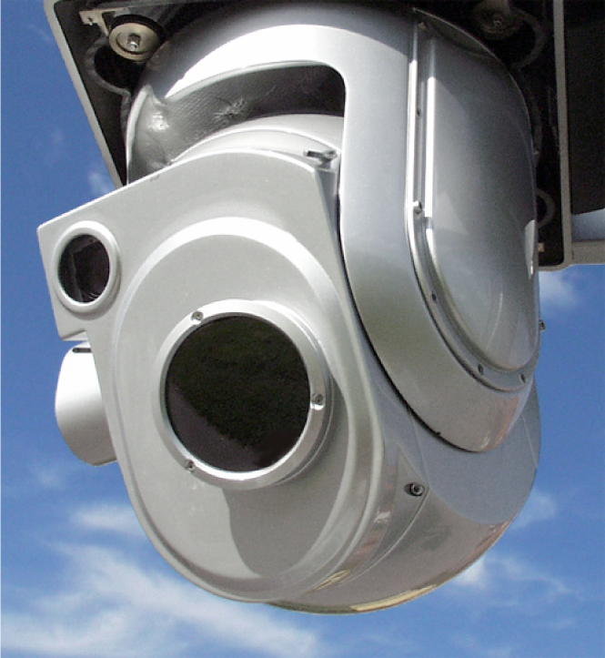
The work is based on Bayesian estimation and search methods, i.e., the search methods are based on the cumulative probability of detection and the target tracking algorithm is based on a particle filter. The exploitation of contextual information, such as maps and terrain information, is highly desirable for the enhancement of the tracking performance, not only explicitly in the target tracker algorithm itself, but also implicitly by improving the sensor management. In this work, the road constrained target assumption is an important aspect of the problem formulation, and this assumption is used extensively to improve both tracking and planning. In this work a single platform with a single pan/tilt tele-angle camera is considered, Figure 1.

An alternative and interesting setup is when a second, possibly fixed, wide-angle camera provides points of interest for the tele-angle camera to investigate. Such setup will probably lead to better performance, but the planning problem will still be similar to the one we are considering in this article and therefore we think that our problem is still very relevant.

The main contributions of this study are:

• Search theory and multi-target tracking are large, but separate, research areas. The problem where search and target tracking are combined has received much less attention, especially in vision-based applications. One of the objectives of this study is to fill this gap.
• There are few studies that examines both high-level and low-level aspects of tracking, planning and searching. In this paper, the state-machine framework adopted uses sub-blocks that achieve low-level tracking, planning and searching tasks while a high-level decision maker chooses among these sub-tasks to obtain an overall situational awareness.
• A useful utility measure for the combined search and target tracking performance is proposed.
• The use of road networks has been used widely to improve the tracking performance of road-bound targets, but in this study we are also utilizing the road network for improved search performance.
• We investigate the effect of the multi-target assumption on the search and show that it results in the same planning scheme as in the single target case.
• There are few studies where both PFs and PMFs are examined. We show the utilization of each algorithm and discuss the merits and the disadvantages with the appropriate applications.

1.1. Background and Literature Survey

Sensor management aims at managing and coordinating limited sensor and system resources to accomplish specific and dynamic mission objectives [3,4]. Algorithms and methods solving realistic sensor management problems are computationally very demanding, since realistic models of the environment, sensors and platforms are very complex due to the nonlinear and stochastic properties of the world. The optimal solution is usually impossible to find, but in practice this is not critical since there is in general a large number of suboptimal solutions that are sufficiently good. However, the problem of finding a good suboptimal solution is still difficult.

A common assumption, utilized also in this work, is that the system can be modeled by a first-order Markov process, i.e., given all of the past states, the current state depends only on the most recent. A Markov Decision Process (MDP) [5,6] is a sequential decision problem defined by a state set, an action set, a Markovian state transition model and an additive reward function. MDP problems can be solved by using Dynamic programming techniques, e.g., the value iteration algorithm [7,8]. In an MDP the current system state is always known. The case where the system state variables are not fully observable is called the Partially Observable MDP (POMDP). The POMDP problem can be transformed to an MDP where the state of the MDP is the sufficient statistics, also called belief state. The belief state is updated according to recursive Bayesian estimation methods. Usually the state space, action space and observation space are assumed to be finite in a POMDP problem.

One of the first algorithms for an exact solution to POMDP was given by Sondik [9]. More efficient exact solvers have been developed, but still only very small problems can be solved optimally. However, different suboptimal methods have also been proposed (see e.g., [10–12]). The suboptimal methods usually approximate the belief space or the value function or both. The development of faster computers with more memory is also one reason to the increased interest into POMDP problems recently.

In receding horizon control (RHC) only a finite planning horizon is considered. The extreme case is myopic planning where the next action is based only on the immediate consequence of that action. A related approach is roll-out where an optimal solution scheme is used for a limited time horizon and a base policy is applied beyond that time point. The base policy is suboptimal, but should be easy to compute. He and Chong [13] solve a sensor management problem by applying a roll-out approach based on a particle filter. Miller et al. [14] propose a POMDP approximation based on a Gaussian target representation and the use of nominal state trajectories in the planning. They are applying the method to a UAV guidance problem for multiple target tracking. He et al. [15] represent the target belief as a multi-modal Gaussian which is exploited in the planning of a tracking problem with road-constrained targets.

One suboptimal approach is to approximate the original problem with a new problem where some theoretical results in planning and control can be applied that makes the problem simpler to solve. One example in the sensor management context is when multi-target tracking planning problems are treated as a multi-armed bandit (MAB) problem (see [4] for a survey). A classical MAB problem contains a number of independent processes (called machines or bandits). An operated machine generates a state dependent reward. The planning problem is to select the sequence of operated machines to maximize the expected return. The problem can be solved by dynamic programming, but it can be shown that a reward index policy is optimal. Thus, the Gittins index (named after its inventor) can be computed independently for all machines and then the optimal policy is to operate the machine with largest index. In sensor management this problem is used in multi-target tracking applications, similar to the problem in this article, where each machine is a target and the problem is to decide which target to update. However, one major disadvantage with the MAB formulation is the assumption that the state of all non-operated machines must be frozen. This is an unrealistic assumptions in target tracking where the targets are moving. There are attempts to overcome this by considering restless bandits [16,17]. In multi-function radar applications a scheduling algorithm is needed to schedule different search, tracking and engagement functions. Many algorithms are based on the MAB problem formulation, but there are also other approaches (see [18] and the references therein). In applications with vision sensor and a moving sensor platform the MAB formulation is not suitable since switching between different targets cannot be performed instantaneously. There are MAB variants where a switching penalty is included, but this violates the optimality of the index policy.

Search theory is the study of how to optimally employ limited resources when searching for objects of unknown location [19,20]. Search problems can be broadly categorized into one-sided and two-sided search problems. In one-sided search problems the searcher can choose a strategy, but the target cannot—in other words, the target does not react to the search. In two-sided search problems both the searcher and the target can choose strategies, and this is related to game theoretical methods. In this work only one-sided search problems are considered.

The elements of a basic search problem are: (a) a prior probability distribution of the search object location; (b) a detection function relating the search effort and the probability of detecting the object given that the object is in the scanned area; (c) a constrained amount of search effort; and finally (d) an optimization criterion representing the probability of success. There are two common criteria that are used in search strategy optimization. One criterion is the probability of finding the target in a given time interval and the other criterion is the expected time to find the target.

The classical search theory, as developed by Koopman et al. [21], is mainly concerned with determining the optimal search effort density for one-sided problems, i.e., how large fraction of the available time should be spent in each part of the search region given a prior distribution for the target location. Much research has been done based on the early work by Koopman; people have investigated different types of detection functions, different search patterns, more general target prior distributions, moving targets and moving searchers (see e.g., [22–24]). There are several recent papers considering a (multi) UAV search for targets using some Bayesian approach, see for instance Bourgault et al. [25] and Furukawa et al. [26]. A common search approach is to represent the target density by a discrete fixed probability grid, and the goal is to maximize the number of detected targets and the search performance is represented by a cumulative probability of detection. In recent years particle mixtures have also been used to represent the target probability density in search and rescue applications (see e.g., [27–30]). In this work two different filters will be used, similar to the approach in [31]. A grid based filter is used for hypothesized but undiscovered targets and once a target is detected it is represented by a particle filter [32].

Classical multi-target tracking consists of three sub-problems; detection, association, and estimation [33,34]. There are different detection approaches; boosting is one popular and powerful method (see [1] and the references therein). An alternative for dynamic targets is optical flow techniques [35]. Target tracking with road network information requires methodologies which can keep the inherent multi-modality of the underlying probability densities. The first attempts [36–38] used the jump Markov (non)linear systems in combination with the variable structure interacting multiple model (VS-IMM) algorithm [39,40]. Important alternatives to IMM based methods appear in [41,42] which propose variable structure multiple model particle filters (VS-MMPF) where road constraints are handled using the concept of directional process noise. In [43] the roads are 3D curves represented by linear segments and the road network is represented as a graph with roads and intersections as the edges and nodes, respectively. The position and velocity along a single road are modeled by a standard linear Gauss–Markov model. Since the particle filters can handle nonlinear and non-Gaussian models, the user has much more freedom than in Kalman filter and IMM modeling. In this work the road target tracking approach in [44] is used, but the association problem is ignored by assuming good discrimination among the targets.

1.2. Outline

The sensor management problem considered in this work is presented in Section 2. A utility measure for evaluating the combined search and target tracking performance is described and a basic example to illustrate its advantages is given. A planner framework based on a state-machine is proposed to handle the complex planning problem and an overview of this planner is also given in Section 2. In Section 3 some fundamental concepts of estimation and search are given and these results are used in later sections. Sections 4 and 5 describe the particle filter (PF) and the point mass filter (PMF), respectively, and how they can be used in search applications. Section 6 returns to the state-machine planner and more detailed descriptions of the planning modes are given together with a presentation of the high-level planner. Section 6 ends with a simulation example where the whole planning framework is applied. Finally in Section 7 some conclusions are drawn. The Appendices collect detailed descriptions of the system model.

2. The Multiple Target Search and Tracking Problem

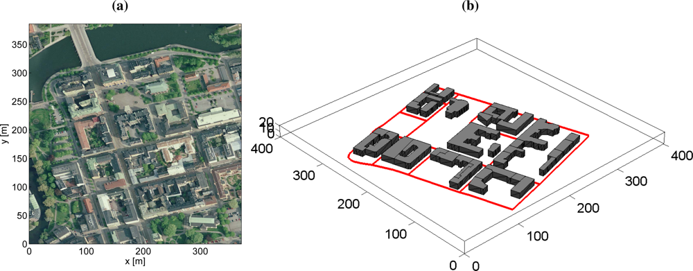
The planning problem in this study is to search for road targets and keep track of discovered targets by controlling the pointing direction of a gimballed vision sensor and the UAV trajectory. The vision sensor has a limited field-of-view (FOV) which makes it unlikely that more than one target can be observed at the same time. One tracking filter is used for each detected target since the targets are assumed to be uncorrelated. The association problem is also ignored, since perfect discrimination is assumed. The surveillance area used in the simulations in this article is shown in Figure 2.

In this section, first the overall objective function is presented in order to evaluate different approaches to the planning problem, and then the general planning problem is described. The section ends with an overview of the planner that is proposed to solve the problem.

2.1. Objective Function

The objective function outputs a scalar such that different plans can be compared, i.e., the better the plan is, the higher is the objective function value. Thus, the objective function must capture what we think is a good planning result. The number of detected targets and the size of the detected targets uncertainty are two obvious properties that say something about the success of the planning. However, how these properties are combined into a scalar objective function is an open problem. For instance, minimizing the uncertainty of discovered targets and maximizing the number of discovered targets are in conflict. In some cases the user prefers a conservative strategy where it is important that a detected target is not lost, and in other cases the user might not care if the target is lost or not, where it is the number of discovered targets that matters.

Consider the uncertainty measure tr P^j where P^j is the state covariance matrix of target j. The reward function −∑_j tr P^j is unbounded from below and lost targets will dominate. However, an information measure like ∑_j det(P^j)⁻¹ does not have that problem. On the other hand, the information value decreases quickly when the target is not visible and this rewards very conservative behavior where the search for new targets is not encouraged.

To summarize, we want a reward function with the following properties:

• It increases with each observation.
• It does not decrease unlimited for unobserved or lost targets, i.e., each target should have a limited influence.
• It should favor strategies that find many targets.
• It should give a fair compromise between splitting the observation resource among the different targets.

We propose the following reward function:

$$\sum _{j=1}^{M_t}{e}^{-\alpha \hspace{0.17em}\text{tr}\hspace{0.17em}{P}^j}$$

(1)

where M_t is the number of targets. Each term e^{−α tr Pj} is a monotonically decreasing function of the uncertainty tr Pⁱ and its value is in [0, 1]. The design parameter α can be tuned to achieve a suitable compromise between low uncertainty and high number of targets. For instance, a very small value of α will lead to a measure which is basically counting the number of targets and ignoring the uncertainty. And a value of α around 0.5 will be similar to the information measure above where the uncertainty dominates over the number of targets. Note that the reward function (1) depends on the statistics of the targets at a single time step. For obtaining the overall cost function to be used in the planning, reward values (1) at each time step are going to be summed over the planning horizon using appropriate weights.

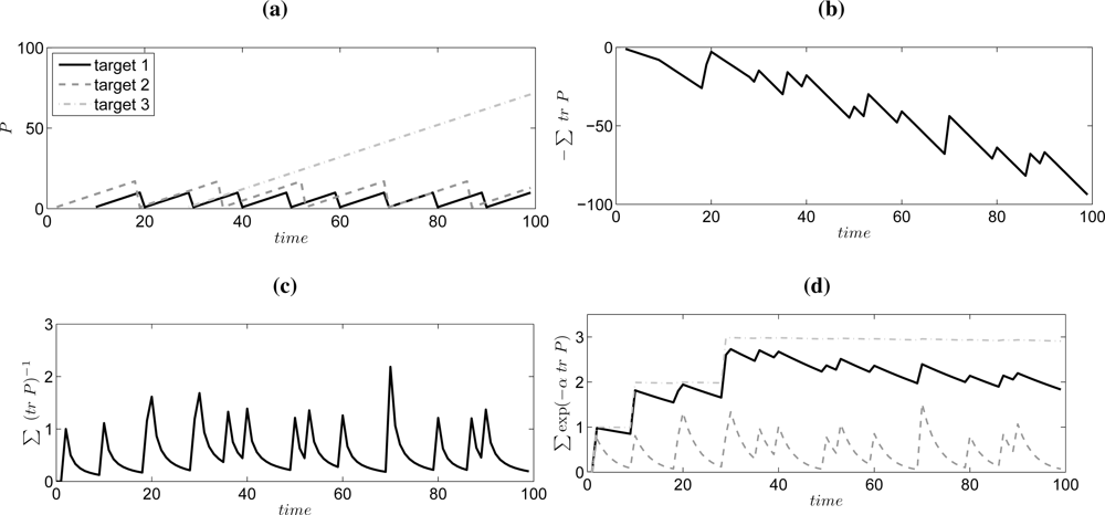
Example 1 (Reward Function Comparison) To illustrate the discussion in this section we will here consider a 1D example with three targets. Let$P_t^j$ = Var(x_t) be the variance of target j at time t. For a random walk target model x_t+1 = x_t + w_t, w_t ∼ $𝒩$ (0, Q), the variance grows as$P_{t+1}^j=P_t^j+Q$ if no observation is available at time t +1. If an observation y_t+1 is available then the observation update step is$P_{t+1}^j:=P_{t+1}^{j}R/(P_{t+1}^j+R)$ according to the Kalman filter covariance update equation given that the observation model is y_t = x_t +e_t, e_t ∼ $𝒩$ (0, R). To summarize, the uncertainty grows linearly when no observation is available, and the uncertainty becomes close to the lower bound when an observation is available.

This behavior is illustrated in Figure 3 where the variances of the three targets are shown in Figure 3(a). Target 1 is re-discovered every 10th time step, target 2 is rediscovered every 17th time step, and target 3 is only observed once at time t = 28. The reward functions are also shown for three different measures. The minus sum of the variance is shown in Figure 3(b), and here we can see the that the uncertainty of target 3 is dominating and this influence will be unbounded. An information measure, defined as sum of the inverse of the variance, is shown in Figure 3(c) and here we do not have the problem with unbounded influence of target 3. On the other hand, the information value decreases quickly when the target is not observed, so in principle it is better to stay with a discovered target and not look for others. Finally, our proposed reward function is shown in Figure 3(d) for three different values of α. For α = 0.001 the reward function is basically the number of detected targets. α = 0.3 gives a similar look as the information utility, and α = 0.02 is a nice compromise between number of detected targets and the information of each target.

The performance is in this work computed as

$$V(t)=\sum _{j=1}^{M_t}{e}^{-\alpha \hspace{0.17em}\text{tr}\hspace{0.17em}[P_t^j]xy}$$

(2)

where [ $P_t^j$]_xy is the xy-position part of the state covariance matrix of target j at time t and M_t is the number of targets at time t. To achieve an overall measure considering all future time instants, a weighted summation over time can be computed as

$$\overline{V}=\sum _{t=0}^{\infty }\gamma (t)V(t)=\sum _{t=0}^{\infty }\gamma (t)\sum _{j=1}^{M_t}{e}^{-\alpha \hspace{0.17em}\text{tr}\hspace{0.17em}{[P_t^j]}_{xy}}$$

(3)

where γ(t) is either the discount function γ(t) = γ^t, 0 < γ < 1 for an infinite-horizon version, or γ(t)=1 for t = 0, 1, ..., r and 0 otherwise for a finite-horizon version.

2.2. The Planning Problem

Assume, without loss of generality, that the planning is performed at time t = 0. The dynamic models of the UAV platform and the gimbal are given in Appendices A.1–A.2 and the augmented model is represented as $x_{t+1}^s=f^s(x_t^s,u_t)$ where $x_t^s$ contains the augmented UAV and gimbal states and the control signal contains three elements u_t = ( $u_t^{\varphi }$, $u_t^{\theta }$, $u_t^{\phi }$)^⊤ that are controlling azimuth (ϕ) and inclination (θ) angles of the gimbal and the heading (φ) of the UAV. It is assumed that the targets are uncorrelated and the motion of a single target j on the road network (Appendix A.3) is represented by $x_{t+1}^j=f^j(x_t^j,v_t^j)$ where the process noise $v_t^j$ is distributed according to some model dependent on $x_{t-1}^j$. Note that the targets are not tracked explicitly in the image plane, but relative the road network represented in a global Cartesian reference frame. A detection $y_t^j$ of target j is used to update the target probability density via the bearings-only observation model in Appendix A.4 here represented as $h(x_t^j;x_t^s)+e_t^j$ where $e_t^j$ is white Gaussian noise. A detection is obtained at time t with the probability

$$P_D(x_t^j;\hspace{0.17em}{x}_t^s)=\prod _{i=r,f,o}{P}_D^i(x_t^j;\hspace{0.17em}{x}_t^s).$$

(4)

where the letters r, f, o represent range, field-of-view and occlusion respectively, see Appendix A.5 for details.

The goal of the planning is to find a control law u_t(I_t) that maximizes the objective function. The control law is a function of all available information I_t at time t. The overall optimization problem can be summarized as

$$\begin{array}{ll}\hfill \underset{u_t(I_t),\hspace{0.17em}t=0,1,\dots }{\text{max}}& E\hspace{0.17em}\left\{\sum _{t=0}^{\infty }\gamma (t)\sum _{j=1}^{M_t}{e}^{-\alpha \hspace{0.17em}\text{tr}\hspace{0.17em}{[P_t^j]}_{xy}}\right\}\hfill \\ \hfill \text{s.t.}& u_t(I_t)\in 𝒰\hfill \\ \hfill & x_{t+1}^s=f^s(x_t^s,\hspace{0.17em}{u}_t(I_t))\hfill \\ \hfill & x_{t+1}^j=f^j(x_t^j,\hspace{0.17em}{v}_t^j),\hspace{0.17em}j=1,\hspace{0.17em}2,\hspace{0.17em}\dots ,\hspace{0.17em}{M}_t\hfill \\ \hfill & y_{t+1}^j=\{\begin{array}{ll}h(x_{t+1}^j;\hspace{0.17em}{x}_{t+1}^s)+e_{t+1}^j,\hfill & \text{if}\hspace{0.17em}\text{detection}\hfill \\ \varnothing ,\hfill & \text{if}\hspace{0.17em}\text{no}\hspace{0.17em}\text{detection}\hfill \end{array}\hfill \\ \hfill & t=0,\hspace{0.17em}1,\hspace{0.17em}2,\hspace{0.17em}\dots \hfill \end{array}$$

(5)

where the initial state $x_0^s$ and the distributions for $x_0^j$, $v_t^j$ and $e_t^j$ are given. In a way this planning problem is a POMDP, but not in the classical way since the state space, the measurement space and the action space are all continuous and not discrete.

2.3. State-Machine Framework

The planning problem (5) is very complex and, as far as we know, there is no known approach that can tackle this problem in a suitable way. Even if there was a suitable and sophisticated approach available, it is not certain that treating the problem as a monolithic problem is a good idea, since the planning process will then be a black-box that is hard to understand from a user’s perspective.

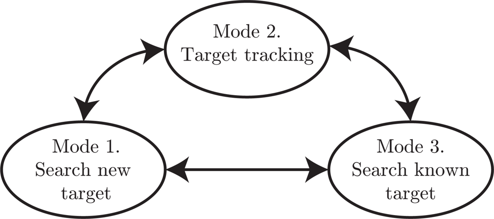
A state-machine approach is instead proposed to simplify the planning problem. The state-machine contains three major states, representing three different planning modes, see Figure 4. Furthermore, a high-level planner is deciding which state/mode is active. Thus, the proposed planner solves an approximation of the general infinite-horizon planning problem (5).

• Mode 1: Search for new targets. In this search mode the roads are explored to discover new unknown targets. This search will stop once a target is detected and a mode transition to mode 2 will be performed. To know which road segments that have been searched, a probability grid on the roads is maintained. In the update step the weights are decreased for grid points in the current sensor footprint, see Section 5 for details.
• Mode 2: Target tracking. When the target tracking mode is active it is assumed that a target has been detected in the current sensor frame. The task of this mode is just to keep track of the current target in the sensor view. The default case in this work is that the target tracking mode is active for a fixed number of time steps, and then the high-level planner decides a transition to either mode 1 or mode 3.
• Mode 3: Search for known target. When a previously discovered target is not observed for some time, its position uncertainty grows. Thus, when the target must be re-discovered it might not be possible to point the sensor in the correct direction since the uncertainty is too large. In such cases, this mode will be active to perform a search on road segments where the target is likely to be.
• High-level planner. The high-level planner decides which mode is active. Basically, the task is to decide if any known target needs to be re-discovered and updated, or if there is time to conduct search for new targets. There is an obvious conflict in this problem, when one target is tracked, or searched for, then the uncertainty of the other targets will grow, and with increasing uncertainty the expected search time for re-discover is also increasing.

The tracking Mode 1 is quite straightforward to develop, and the task is to make sure the target is centered in the sensor frame. Modes 2 and 3 and the high-level planner is the main topic of this article. First some basics of estimation and search will be presented in Section 3, then the particle filter used for target density estimation is presented in Section 4. The approach used in Mode 1 is described in Section 5. The whole state-machine is again considered in Section 6 where also the high-level planner is described in detail. Some simulation examples are presented along the way to the final results in Section 6.6.

3. Elements of Single Target Bayesian Search

In this section, the search objective function, which will be the basis of all optimization objective functions used throughout this work, is derived. First we present the Bayesian recursions which will serve as a starting point for the calculation of the objective function. Then the derivation of the search criterion is presented.

3.1. The General Estimation Solution

The aim of this section is to introduce the recursive state estimation theory [45]. Let x_t denote the state of a target at time t and let y_t be an observation of the target at time t. Assume that the target state evolution can be represented as p(x_t+1|x_t) and let the observation model be expressed via the likelihood function p(y_t|x_t). Let y_1:t = {y₁, y₂, ..., y_t} denote the set of all observations up to and including time t. The general state estimator is given by Bayes rule

$$p(x|y)=\frac{p(y|x)p(x)}{p(y)}$$

(6)

and can be expressed as the update formula

$$p(x_t|y_{1:t})=p(x_t|y_t,\hspace{0.17em}{y}_{1:t-1})={\eta }_t^{-1}p(y_t|x_t)p(x_t|y_{1:t-1})$$

(7)

and the one step ahead prediction

$$p(x_t|y_{1:t-1})=\int p(x_t|x_{t-1})p(x_{t-1}|y_{1:t-1})d{x}_{t-1}.$$

(8)

The normalizing factor η_t can be calculated as

$${\eta }_t=p(y_t|y_{1:t-1})=\int p(y_t|x_t)p(x_t|y_{1:t-1})d{x}_t.$$

(9)

The above equations represent the so-called Bayesian filter and there are only few cases when it is possible to derive the analytical solutions for them. One case is the linear Gaussian case, leading to the well known Kalman filter (KF). In the general case, numerical approximations are necessary and one popular technique is to approximate the target density p(x_t|y_1:t) with a particle mixture as in the particle filter (PF), or with a point grid as in the point mass filter (PMF).

3.2. Cumulative Probability of No Detection

As in the estimation theory introduction, assume that x_t is the state vector of the target at time t. Let y_t be an observation of the target at time t, and if y_t = ∅ no detection was obtained. Denote the probability of detection as p(y_t ≠ ∅|x_t) and the probability of no detection by its complement p(y_t ≠ ∅|x_t) = 1 − p(y_t ≠ ∅|x_t). Now the probability of no detection at time t conditional on the observations y_0:t−1 is found by the marginalization

$$p(y_t=\varnothing |y_{0:t-1})=\int p(y_t=\varnothing |x_t)p(x_t|y_{0:t-1})d{x}_t$$

(10)

where p(x_t|y_0:t−1) is the prediction density from the Bayesian filter. Define

$${\lambda }_t\triangleq p(y_t=\varnothing |y_{0:t-1}=\varnothing )$$

(11)

and the joint probability of no detection from time 0 to time t can be expressed as the product

$${\mathrm{\Lambda }}_{0:t}\triangleq p(y_{0:t}=\varnothing )=\prod _{i=0}^t{\lambda }_i.$$

(12)

In this work the cumulative probability of no detection Λ_0:t will be used as the cost function. Note that λ_t is the normalizing constant in the observation update step (9). The cumulative probability that the target is detected at time t or before is the complement to Λ_0:t, i.e.,

$${\mathrm{\Pi }}_{0:t}=p(y_{0:t}\ne \varnothing )=1-p(y_{0:t}=\varnothing )=1-{\mathrm{\Lambda }}_{0:t}.$$

(13)

Note that Π_0:t is non-decreasing.

Now consider the case when λ_i ≜ 1 − μ are equal for all i = 0, 1, ..., t.

$${\mathrm{\Pi }}_{0:t}=1-{(1-\mu )}^t.$$

(14)

For a large number of t the cumulative probability of detection (13) can be approximated (using the binomial theorem) by the exponential distribution [46]

$${\mathrm{\Pi }}_{0:t}=1-e^{-\mu t}.$$

(15)

4. Single Road Target Search based on a Particle Filter

A common choice to represent the target probability density in search applications is to use a grid representation of the world where the target might be [25]. Each cell in the grid has a certain weight representing the probability that the target is in that cell. An alternative is to use a particle mixture. This representation has some similarities with a grid based representation, but also some important differences. In the next subsection the particle filter Gordon et al. [47], which is a Bayesian filter that uses a particle mixture, is briefly described and some further comparisons between the grid and the particle representations are made. Then the calculation of the search criterion based on the particle mixture is shown and finally some simulation examples are presented.

4.1. Particle Filter

In a particle filter Arulampalam et al. [32], Gustafsson [48] the target density p(x_t|y_1:t) is approximated by a particle mixture, containing N particles ${\{x_t^{(i)}\}}_{i=1}^N$ and their corresponding importance weights ${\{w_t^{(i)}\}}_{i=1}^N$. This approximation is expressed as

$$p(x_t|y_{1:t})\approx \sum _{i=1}^N{w}_t^{(i)}\delta (x_t-x_t^{(i)})$$

(16)

where

$$\sum _{i=1}^N{w}_t^{(i)}=1,\hspace{0.17em}\hspace{0.17em}\hspace{0.17em}\hspace{0.17em}\hspace{0.17em}{w}_t^{(i)}\ge 0,\hspace{0.17em}\hspace{0.17em}\hspace{0.17em}\hspace{0.17em}\hspace{0.17em}\hspace{0.17em}\hspace{0.17em}\hspace{0.17em}\hspace{0.17em}\hspace{0.17em}\hspace{0.17em}\hspace{0.17em}\hspace{0.17em}\hspace{0.17em}\hspace{0.17em}\forall i$$

(17)

and δ(·) is the Dirac delta distribution. This approximation is very suitable for calculating the integral in (8) and it can be shown that this approximation converges to the true solution as the number of particles goes to infinity for the details on particle filtering. There are different types of particle filters, perhaps the most straightforward version is the Bootstrap particle filter (BSPF) that is used in this work. In BSPF the so-called proposal density is selected as the state transition model p(x_t+1|x_t). The filter recursion (7) and (8) can, in the BSPF case, be expressed as

$$\begin{array}{l}{w}_{t|t}^{(i)}\propto p(y_t|x_t^{(i)})w_{t|t-1}^{(i)},\hspace{0.17em}\hspace{0.17em}\hspace{0.17em}\hspace{0.17em}\hspace{0.17em}\hspace{0.17em}\hspace{0.17em}\hspace{0.17em}\hspace{0.17em}\sum _{j=1}^N{w}_{t|t}^{(j)}=1\\ x_t^{(i)}\sim p(x_t|x_{t-1}^{(i)})\end{array}$$

(18)

Furthermore, a resampling step is needed to prevent degeneration.

4.2. Calculation of the Cost Function with the PF

The search objective function based on the cumulative probability of non-detection (12) and the particle mixture representation (16) is presented. Assume that the planning horizon is n and that the sensor platform trajectory $x_t^s$, t = 1, 2, ..., n is given.

• Let t = 1. Initialize the particle mixture weights used in the planning as ${\overline{w}}_0^{(i)}:=w_{0|0}^{(i)}$ for i = 1, 2, ..., N where ${\left\{w_{0|0}\right\}}_{i=1}^N$ is the set of current target probability density in the tracking filter.
• Simulate the evolution of the particles according to the target model

  $$x_{t+1}^{(i)}=f(x_t^{(i)},\hspace{0.17em}{v}_t^{(i)}),\hspace{0.17em}\hspace{0.17em}i=1,\hspace{0.17em}2,\hspace{0.17em}\dots ,\hspace{0.17em}N.$$

  (19)
• Compute the probability of detection, P_D(x_t), and update the target density given a non-detection. Thus, for all particles i, calculate

  $$\begin{array}{r}\hfill P_D(x_t^{(i)})=\text{Pr}(y_t\ne \varnothing |x_t^{(i)},\hspace{0.17em}{x}_t^s)\\ \hfill {\overline{w}}_t^{(i)}=(1-P_D(x_t^{(i)})){\overline{w}}_{t-1}^{(i)}\end{array}$$

  (20)

  and then compute the non-detection probability and normalize the weights according to

  $${\lambda }_t=\sum _{i=1}^N{\overline{w}}_t^{(i)},\hspace{0.17em}\hspace{0.17em}\hspace{0.17em}{\overline{w}}_t^{(i)}:=\hspace{0.17em}{\lambda }_t^{-1}{\overline{w}}_t^{(i)}.$$

  (21)
• Set t := t +1. If t ≤ n, then go to step (ii), otherwise go to the next step.
• Set the cost function value as the cumulative probability of non-detection

  $$c({\{x_k^s\}}_{k=1}^n)={\mathrm{\Lambda }}_{1:n}=\prod _{k=1}^n{\lambda }_k.$$

  (22)

When running this algorithm several times, e.g., in an optimization routine, it is possible to pre-compute the particle trajectories of the target to save computational time since the target is independent of the actions of the searcher.

Example 2 (Single Target Search with PF) In this simulation example a UAV with a gimballed vision sensor searches for a lost moving target with known Gaussian prior distribution. The control signals are the heading of the UAV and the azimuth angle of the vision sensor. The main search algorithm is quite simple and essentially it is a receding horizon control (RHC) approach with a gradient based optimization routine to maximize the cumulative probability of detection. The particle filter is used to compute the posterior density of the target and the particle mixture is also predicted in the cumulative probability of detection computations.

The detection likelihood of the vision sensor is range dependent and the pinhole camera model is used to compute the probability of detection depending on the pointing direction, see Appendix A.5. The nearly constant speed motion model in Appendix A.1 is used as the target motion model. The states of this model are the Cartesian position, the speed in the xy-plane and the heading. The same motion model is also used as the UAV model, but no noise is added and the navigation error is ignored. The turn rate of the vehicle is the control signal and there is a constraint on the turn rate, i.e., on the minimum path radius of the UAV. The second control signal is the rotational speed of the pan angle. The pan dynamics is modeled as a simple first order model with input constraints, see Appendix A.2. The number of optimizations parameters are 4 for each control signal and the active-set approach of the standard toolfmincon is used in Matlab Optimization Toolbox.

Three snapshots of the simulation are shown in Figure 5. The target density vanishes where the sensor is pointing and after the resampling step the number of particles decreases in those areas, but increases everywhere else. Since the target is not detected, the particle cloud spreads out more and more. However, when the target is found (not shown here) the particle cloud will shrink to a small area around the detection location.

5. Multi-Road-Target Search Based on PMF

In this section, we are going to investigate the search problem under the assumption that multiple targets exist in the search region. First, we are going to generalize the single target search case based on the cumulative probability of no detection to the case of multiple targets, where it will be shown that the assumption of multiple targets will result into the same search plan as the single target case. Based on this result, we will propose a model for representing the target probability density of undiscovered targets. The goal of this filter is not to track the state of a discovered target; instead this filter will be used to model which areas have been searched. Since the density will be rather flat on the whole road network, the point-mass filter (PMF) will be used, i.e., a grid will be defined on the road network and the corresponding weights of the grid points represent the probability of at least one target in that location. This section ends with a simulation showing a target search example.

5.1. Generalization of the Single Target Search to Multiple Targets

We here consider the generalization of the methodology in the previous sections to the case that multiple targets exist in the search region. We assume the availability of a discrete distribution over the number of targets (called cardinality distribution [49]). Suppose we call this distribution as P_T (M), where M is the number of targets. Then we assume that the targets in the prediction horizon have the following multi-target likelihood function

$$p_t(\{x_t^1,x_t^2,\hspace{0.17em}\cdots ,\hspace{0.17em}{x}_t^M\})\hspace{0.17em}\triangleq \hspace{0.17em}{P}_T(M)\prod _{i=1}^M{p}_t(x_t^i)$$

(23)

where p_t(·) is a given density function over the target state space and will be selected as the predicted target density in our application, i.e., p_t(·)= p(x_t|y_0:t−1 = ∅). The processes which have the likelihood function of the form (23) are called independent identically distributed (i.i.d.) cluster processes in general [49]. The following theorem gives the generalization of the cumulative probability of no detection for the multiple target case.

Theorem 1 (Multiple target cumulative probability of no detection) The cumulative probability of no detection for the multiple target case is given by

$$P_{ND}(t)\triangleq G_T\left(\prod _{i=1}^t{\lambda }_i\right)$$

(24)

where the function G_T (·) is defined as

$$G_T(x)\triangleq \sum _{n=0}^{\infty }{P}_T(n)x^n.$$

(25)

The proof of the theorem is given in Appendix B for the sake of clarity.

In probabilistic terms, the function G_T (·) is the probability generating function corresponding to P_T (·) ([50]; Section 4.8). It is in general a monotonically non-decreasing function of its argument in the interval [0, 1] and G_T (0) = 0 and G_T (1) = 1 ([50]; Section 4.8).

By Theorem 1, the search problem for the multiple target case becomes obtaining the search plan that minimizes $G_T\left({\prod }_{i=1}^t{\lambda }_i\right)$, which is equivalent to the minimization of the argument ${\prod }_{i=1}^t{\lambda }_i$ since G_T (·) is monotonic. This shows that the multiple target search using the cumulative probability of no detection is equivalent to the single target search which uses the same cost function.

5.2. Point-Mass Filter

In a point-mass filter (PMF), a.k.a. grid method, the target probability density is approximated with a number of grid points. This grid representation in a PMF is actually similar to the particle representation in the PF, but the grid points in the PMF are stationary and defined deterministically while the particles in the PF are stochastic and non-stationary. In the PMF [32,51] the continuous probability density p(x_t|y_1:t) is discretized. The general filter recursion (7) and (8) in Section 3.1 can then be approximated as

$$\begin{array}{ll}\hfill p(x_t^{(i)}|y_{1:t})=& {\eta }_t^{-1}p(y_t|x_t^{(i)})p(x_t^{(i)}|y_{1:t-1})\hfill \\ \hfill p(x_t^{(i)}|y_{1:t-1})=& \sum _{j=1}^{N}p(x_t^{(i)}|x_{t-1}^{(j)})p(x_{t-1}^{(j)}|y_{1:t-1}){\mathrm{\Delta }}^{(j)}\hfill \\ \hfill {\eta }_{t=}& \sum _{j=1}^{N}p(y_t|x_t^{(j)})p(x_t^{(j)}|y_{1:t-1})\hfill \end{array}$$

(26)

and Δ^(j) is computed such that

$$\sum _{i=1}^{N}p(x_t^{(i)}|x_{t-1}^{(j)}){\mathrm{\Delta }}^{(j)}=1.$$

(27)

The advantage of the PF approach compared to this grid filter approach is that the resolution adapts automatically so that high probability regions have higher resolution. Consequently, the advantage of a grid approach is that it has better support in low probability areas compared to a particle mixture that needs a very high number of particles for flat target densities. The particle filter is more flexible in terms of target motion models and even though the PF has problems with high-dimensional state-spaces, it is in general a better choice than the grid approaches for problems with a state-space dimension of 3 and higher. However, for 2D problems the PMF is a nice filter that is straightforward to implement and that can handle multi-modal probability densities. There exist methods for adapting the grid resolution and its spatial spread as a approach to solve the problem of larger state-spaces [51].

5.3. Target Search on a Road Network Grid

Consider a random walk model and an observation model with additive noise

$$x_{t+1}=x_t+v_t,\hspace{0.17em}{v}_t\sim 𝒩(0,\hspace{0.17em}{\sigma }_v^{2}I)$$

(28)

where x_t = [x y] is the 2D location of the target at time t. Let x⁽ⁱ⁾, i = 1, 2, ..., N be the grid points located on the road network and let $W_{t|t}^{(i)}$ be the corresponding weights representing the posterior target probability density p(x_t|y_1:t), i.e., the probability of target being in location x⁽ⁱ⁾ is proportional to the weight $W_{t|t}^{(i)}$ ∝ Pr(x_t = x⁽ⁱ⁾|y_1:t). In the non-detection case the filter update step is

$$W_{t|t}^{(i)}=(1-P_D(x_t))W_{t|t-1}^{(i)}.$$

(29)

The computation of the time update step can be expressed as

$$W_{t|t-1}^{(i)}=\sum _{j=1}^N{P}^{(i,j)}{W}_{t-1|t-1}^{(j)}$$

(30)

where

$$P^{(i,j)}\propto p(x_t^{(i)}|x_{t-1}^{(j)})=𝒩(x_t^{(i)};\hspace{0.17em}{x}_{t-1}^{(j)},\hspace{0.17em}{\sigma }_v^{2}I),$$

(31)

such that

$$\sum _i{P}^{(i,j)}=1,$$

(32)

can be pre-computed. The computation of the cumulative probability of non-detection is basically the same as in the PF case (22), i.e.,

$$\begin{array}{c}c({\{x_t^s\}}_{t=1}^n)={\mathrm{\Lambda }}_{1:n}=\prod _{t=1}^n{\lambda }_t,\\ {\lambda }_t=\sum _{i=1}^N{W}_t^{(i)}.\end{array}$$

(33)

Example 3 (Road Target Search using PMF—Stationary UAV and No Occlusion) The reference aim point is parametrized in road target coordinates and the aim point follows the road with a predefined ground speed. When the aim point is approaching an intersection the different road alternatives are evaluated by comparing the expected cumulative probability with a fixed planning horizon for each possible alternative. The road with the highest value is selected. The sampling time is 0.1 s and the grid resolution is about 5 m. The UAV is stationary and 100 m over ground and the camera field-of-view is 10^° × 7.5^°. The random walk model is used as the target motion model with quite small process noise variance for illustrative purposes (it is easier to see where the search has been conducted in the figures). In practice, a higher value should be used to model moving targets in a better way. Three snapshots of the simulation are shown in Figure 6. An extension of the search planner is a test on the expected cumulative detection probability, if below a certain threshold the whole grid is evaluated for the best location of search. The evaluation is based on the grid weights times the probability of detection function, assuming an unlimited field-of-view camera, and finally a smoothing (Gaussian) kernel is applied. The camera is steered to the grid point with the highest value.

Example 4 (Road Target Search using PMF—Moving UAV and Occlusion) The same target model and grid are used as in previous example, but here the UAV is moving and the occlusion due to the buildings is also included. The UAV model is the nearly constant speed model in Appendix A.1 with the turn rate as the control signal. The UAV is trying to catch a reference point that is a pre-defined distance ahead of the aiming reference point. Which way the UAV reference point will choose at an intersection is similar as in the aim point case, but instead of cumulative probability of detection the grid weights are evaluated. Three snapshots of the simulation are shown in Figure 7. The search is effective and the occlusion of the roads is handled quite well, despite the simple idea of the UAV path control strategy.

An approach where both the path planning and the sensor direction is optimized jointly yields better result, at least in theory. However, in practice such optimization problems become much more complex due to more degrees of freedom. The proposed method, where the aim point and flight path are solved in a sequence, is cheap to compute and easier to understand for a human operator, yet very efficient and robust. Most of the occlusion handling flaws of the proposed method can be solved within the frames of this planning sequence.

6. Multiple Road Target Search and Tracking

In Sections 3–5 some tools are described that will be used here to fill the proposed state-machine planner in Section 2.3 with suitable contents. Now recall the modes described in Section 2.3:

• New target search; search for new targets that have not been discovered before. This mode is further explained in Section 6.1.
• Tracking Tracking; a detected target is followed in the current sensor frame, Section 6.2.
• Known target search; search for an earlier discovered target that is not in the current sensor frame, Section 6.3.

A high-level planner decides which mode will be active (Section 6.4). The outcome of all modes is an aiming reference point and this point is also used the UAV path planner (Section 6.5).

6.1. New Target Search

In this search mode the roads are explored to discover new unknown targets and the grid approach presented in Section 5 is here used. The search will stop once a target is detected and a mode transition to the Target tracking mode will then be performed. The reason for using PMF is the good support all over the surveillance area, but at a cost of that a very simple target motion model must be used due to the curse of dimensionality. In the current case a random walk model is used, which leads to a quite efficient update step of the PMF. A random walk model is of course not a good model of the target motion but still a reasonable choice in this case, since we only need a description of where search has been conducted. The search is performed along one road with a predefined search speed, which is a compromise between rapid coverage and low degree of motion blur in the images. When the search approaches an intersection the best road is selected according to the expected cumulative probability of detection.

6.2. Target Tracking

When the Target tracking mode is active it is assumed that a target has been detected in the current sensor frame. The task of this mode is just to keep track of the current target in the sensor view. If the target is new, a new particle filter is initialized (Section 4.1). The default case in this work is that the Target tracking mode is active for a fixed number of time steps, and after that the high-level planner again decides a transition to either the New target search mode or the Known target search mode. Thus, the transition to and from the Target tracking mode is well specified.

6.3. Known Target Search

When a previously discovered target has not been observed for some time, its position uncertainty has grown. To keep the uncertainty at an acceptable level, the target must be rediscovered on a regular basis. However, the larger the uncertainty is, the longer is the expected search time to find the target again. If the uncertainty is above a certain threshold, the target is considered lost. When the high-level planner decides to re-discover a known target again, a position on the border of the particle cloud is selected and then the particle cloud is swept over. If the particle cloud is spread over several roads, the most probable road is selected, i.e., the road with the highest sum of particle weights. During the search the target density is updated according to the non-detection update rules in Section 4.2.

6.4. High-Level Planner

The high-level planner decides which mode is active. Basically, the task is to decide if any known target needs to be updated and re-discovered, or if there is time to conduct search for new targets. There is an obvious conflict in this problem. When one target is tracked, the uncertainty of the other targets will grow, and with increasing uncertainty the expected search time for re-discovery is also increasing. At some point the uncertainty is so large that the target can be considered lost. At every time step (except when in the Target tracking mode), the planner checks the current status and decides if a mode transition is needed.

The proposed high-level planner relies on a stochastic scheduling result in [53].

Theorem 2 (Maximum Finite-Time Returns) Suppose there are n jobs to be performed sequentially within a fixed time t and assume that job j takes an exponential amount of time with mean 1/μ^j, i.e., P (X^j < t) = 1 − e^{−μj t}, where X^j is the time needed to finish the job. If the job is completed within t are ward of R^j is earned. The expected return by time t is maximized by attempting jobs in decreasing order of μ^jR^j, j = 1, 2, ..., n.

Proof: see [53].

Our problem can also be considered a stochastic scheduling problem where the jobs are to re-discover targets or search for new. However, the expected time to detection is not exponential, but it is a reasonable approximation. Actually, Koopman in the early days of search theory addressed a search problem with a patrol aircraft searching for a ship in open sea and he showed that if an area A is searched “randomly” in a uniform manner then the cumulative probability of having detected the target in the region is an exponential function

$$P_D(z)=1-e^{-zW/A},$$

(34)

where W is the sweep width and z is the track length, see [19]. Also compare with the cumulative detection probability in (15).

A more significant approximation is that the scheduling result above assumes a static setup, but our problem is dynamic since target uncertainties change (grow in general) as time goes by. Thus, a decision must be made on the time step the scheduling will be based on, the most obvious choice is the current time t = 0, but it is also possible to predict the target states and evaluate the result at a certain time t > 0.

It is important to be aware of these approximations when we apply Theorem 2 to our planning problem. First consider a discovered target j with state covariance $P_t^j$. We assume that finding this target takes an exponential amount of time with (inverted) mean

$${\mu }^j={\left(\tau +\frac{4\sqrt{\text{tr}{[P_t^j]}_{xy}}}{\nu }\right)}^{-1}$$

(35)

where τ is a mode transition time due to the dynamics of the gimbal, in this work τ is just a constant. ν is the speed of the footprint on the ground. The second term can be motivated by the following reasoning: The distance from −2σ to 2σ of a one-dimensional Gaussian distribution with variance σ² is 4σ and the time to travel that distance with speed ν is 4σ/ν. In a single road case σ can be approximated by $\sqrt{\text{tr}{[P_t^j]}_{xy}}$.

The reward of rediscovering target j is based on the criterion introduced in Section 2.1:

$$R^j=1-e^{-{\alpha }_P\hspace{0.17em}\text{tr}{[P_t^j]}_{xy}}.$$

(36)

Basically, if the uncertainty is very low, then the reward is close to zero, and vice versa. Furthermore, with the design parameter α_p the user has the possibility to tune the planner into the desired behavior according to the discussion in Section 2.1. It is of course possible to use different α_p values for different targets. To illustrate the behavior of the product μ^jR^j as a function of tr[ $P_t^j$]_xy, the special case

$${\mu }^j{R}^j=\frac{1-e^{-0.1\hspace{0.17em}\text{tr}{[P_t^j]}_{xy}}}{1+\sqrt{\text{tr}{[P_t^j]}_{xy}}}.$$

(37)

where α_p = 0.1, ν = 4 and τ = 1, is shown in Figure 8. The reward is low when the uncertainty of the target is low, but the reward is decreasing after a certain point due to increased search time.

The New target search mode is just defined as an extra “job”, and this alternative is denoted as j = 0. The reward of discovering a new target is simply R⁰ = 1 and the expected (inverted) time for discovering a new target is

$${\mu }^0={\left(\tau +\frac{L}{m\nu }\right)}^{-1}=\frac{m\nu }{m\nu \tau +L}$$

(38)

where L is the total length of all roads in the surveillance area, and m is the expected number of undiscovered targets. Thus, it is now possible to evaluate the New target search mode with different targets in the Search known target mode within the same framework.

The high-level planner is summarized in Algorithm 1.

Algorithm 1 (High-Level Planner: Mode Selection) If a new target is detected in the current frame, the active mode will be the Target tracking mode. Otherwise, the active mode (and possibly target) is decided by the following steps:

• Compute the value

  $${\mu }^0{R}^0=\frac{m\nu }{m\nu \tau +L}$$

  (39)

  where m is the expected number of targets in the surveillance area, τ is a mode transition time constant, ν is the search speed on the road and L is the total length of all roads in the surveillance area.
• Compute the value

  $${\mu }^j{R}^j={\left(\tau +\frac{4\sqrt{\text{tr}{[P_t^j]}_{xy}}}{\nu }\right)}^{-1}\hspace{0.17em}\hspace{0.17em}\hspace{0.17em}(1-e^{-{\alpha }_p\hspace{0.17em}\text{tr}{[P_t^j]}_{xy}})$$

  (40)

  for all targets j = 1, 2,...,M_t. P_xy is the covariance of the target position state and α_p is a design parameter.
• Let

  $$q=\text{arg}\hspace{0.17em}\underset{j=0,1,\dots ,M_t}{\text{max}}{\mu }^j{R}^j.$$

  (41)

  If q = 0 then select the New target search mode, otherwise select the Known target search mode for target q.

The planner is suboptimal in the sense that it evaluates the current state and assumes open loop control over the planning horizon. Moreover, it assumes that all targets will be visited just once. The problem dynamics and the utilization of new measurements are handled by replanning on a regular basis in a RHC manner. One way to improve the high-level planner is to develop a roll-out approach where the proposed planner serves as the base policy.

The assumptions of the proposed method has some similarities with the assumptions made in a multi-armed bandit (MAB) problem. Both approaches assume independent targets and that only one single target is processed at the same time. Moreover, both approaches assume that the targets are not affected by the action of the sensor platform and both simplifies the target dynamics. As mentioned in Section 1.1, the main advantage of a MAB formulation is that the optimal policy is of index type. Algorithm 1 also has this property, since values are computed independently for all alternatives and then the best alternative is given by the largest value. This results in a planner that is cheap to compute yet very efficient, as will be seen in the simulation in Section 6.6. The approximations that are made in the current version of the planner could certainly be improved, but this is left for future work. In particular, alternatives where the target uncertainties are predicted should be examined instead of using the uncertainty of the current time.

6.5. UAV Path Planner

The UAV path planner has already been introduced in Example 4. The UAV model is the nearly constant speed model in Appendix A.1 with the turn rate as the control signal. The flight altitude is constant. The UAV heading rate signal is computed by a basic proportional controller where the heading reference is the direction to a UAV reference point that is at a pre-defined distance ahead of the aiming reference point. All computations are done in the xy-plane, independent of the flight altitude. Which way the UAV reference point will choose in an intersection is decided by evaluating the PMF grid weights for all possible road alternatives and for a given planning horizon. The aiming reference point is of course computed in different ways depending on which mode that is active, but the active mode does not matter for the UAV path planner.

6.6. Simulation Examples: Moving Sensor Platform with Occlusion

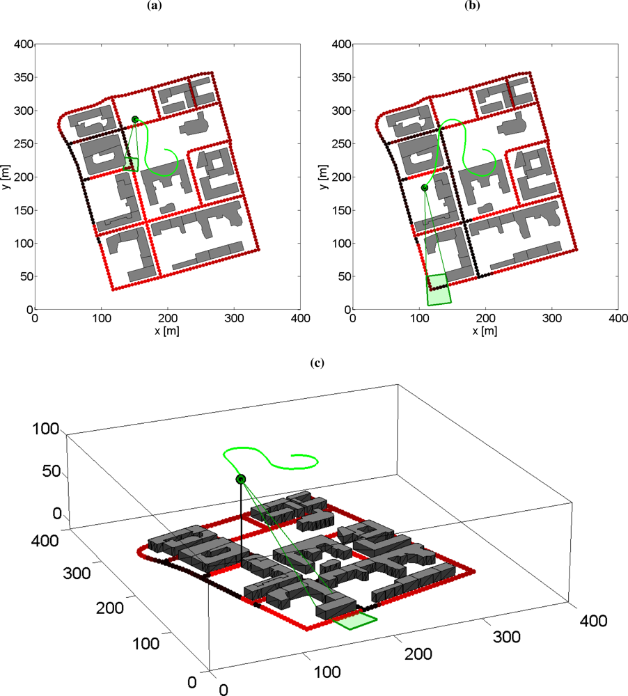
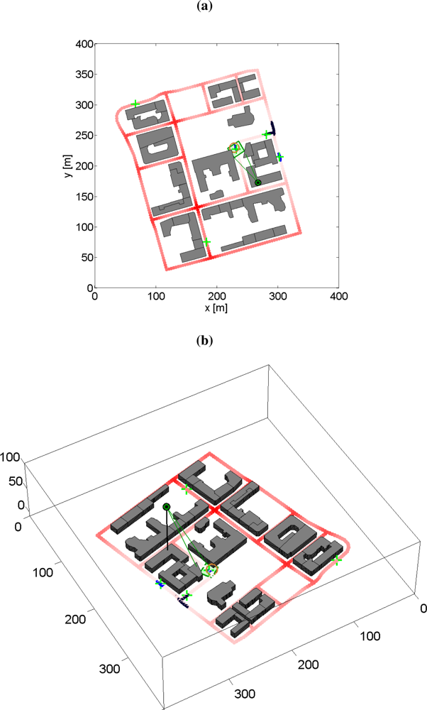
Three simulations are here presented to illustrate the qualitative behavior of the proposed planning method in a multi-target tracking scenario with five moving road targets in an urban area. All targets are initially unknown to the sensor platform. A snapshot from one simulation is shown in Figure 9. (Movies are available, see [52].) The preconditions of the three simulations are the same except for the planner parameter α_p. The value of this parameter is (a) α_p = 10⁻⁶, (b) α_p = 0.002 and (c) α_p = 0.1, respectively.

In Figure 10 it is shown if the planner is searching for new targets or which target it is currently searching for or following. The “new target” row at the bottom represents the search new target mode. Note that all simulations start in this mode since no targets are known initially. The other five rows show which target is active. Black color indicates the search known target mode and and gray color indicates that the target is visible and that the target tracking mode is active.

In case (b), α_p = 0.002, the result is a reasonable compromise between updating known targets and searching for new targets. At the beginning the new target search mode is active most of the time, but as some of the targets are discovered less time is spent on new target search. Case (a), α_p = 10⁻⁶, is an extreme case where the planner just focuses on finding new targets. All five targets are actually discovered in the scenario, but since no explicit attempts to rediscover the known targets are made, the position uncertainty of the discovered targets grows quickly. Case (c), α_p =0.1, is the other extreme case there the planner is very conservative and barely searches for new targets once one target is discovered. Two other targets are detected when they are close to the followed target, and the planner switches focus to one of the new targets.

The simulation results are evaluated by the reward function ${\sum }_{j=1}^5{e}^{-\alpha \text{tr}{[P_t^j]}_{xy}}$ for three different values of α in Figure 11 (solid line). The set of different values for α is the same as the set for α_p used in the three simulations. (Recall the difference between α and α_p. α is used in the reward function (2) and α_p is used in the high-level planner, see Section 6.4.) In the left column of Figure 11 where α =10⁻⁶, the reward function is basically the total number of discovered targets. In the middle column, α = 0.002, the reward can be considered as a soft value of the instantaneous number of tracked target. In the right column, α =0.1, the reward is similar to the information value according to the discussion in Section 2.1. Note that all reward functions are limited by the number of targets, i.e., five in the current case. A scalar measure of the performance can be computed by using (3) (γ = 1). The best performance in each simulation was obtained for the case when α_p = α, which is desirable. However, note that selecting α_p = α will not necessarily give the best planning result according to (3) since the proposed planning method solves an approximation of the general planning problem, but this is a good starting point.

The occlusion problem is handled surprisingly well most of the time, but future work should investigate ways of including the occlusion model explicitly in the UAV path planner and the camera pointing planners.

The conclusion is that the proposed planner solves the general problem (5) in a reasonable way and the behavior of the planner can easily be tuned by the parameter α_p. The best value of this parameter is dependent on the mission goal and the user’s preferences. Although the proposed method is suboptimal there are actually some advantages with this method from a user’s perspective. The planning result from an optimal planner will probably be hard to understand since all objectives and constraints are considered at the same time in a black box manner. It is easier for a human operator to monitor and understand the planning result from a planner with distinct modes.

6.7. Experiences from Real-World Experiments with a Pan/Tilt-Camera

The framework has also been evaluated in experiments with an Axis 233D pan-tilt-zoom network camera and a number of tape following mobile robots, Figure 12. The road network was created by black tape on the ground representing the roads. The target identification step is simplified by the use of markers and a feature recognition algorithm. The Matlab framework, used in the simulations in this article, is also used for tracking and planning, but the control and communication with the camera was implemented in Java.

We got many valuable experiences from the experiments. The well-known saying a system is not stronger than the weakest link is also true for complex tracking systems. Especially the planner is exposed to issues since it is the last part in the navigation-detection-tracking-planner chain. Estimating the position and orientation of the camera is very important, and even more important when the tracker is using prior information (e.g., a road map) given in global world coordinates. Missed detections, false alarms and wrong associations may also have severe impact on the target tracking filter, so when evaluating the planner result in a real world application, it is important to be aware these problems. If the information that is fed into the planner is wrong or insufficient, then the planning result will of course also be bad.

It is also very important to have suitable system models. The model choice is often a compromise: the model can not be too complex for computational reasons and it can not be too simplified since the results would then be irrelevant. In particular, the detection probability model is a main component in this study. It is tempting to ignore effects like motion blur and atmospheric disturbances in the simulations, but for a successful real-world application it is important to be aware of such phenomena. In general, it is extremely difficult to obtain a model of the absolute detection performance for vision sensors (see [54]).

7. Conclusions

This article considers a sensor management problem where a number of road bounded vehicles are monitored by an unmanned aerial vehicle (UAV) with a gimballed vision sensor. The problem is to keep track of all discovered targets, and simultaneously search for new targets, by controlling the pointing direction of the camera and the motion of the UAV. The motion of the targets (e.g., cars) are constrained by a road network which is assumed to be prior information.

One key to a successful planning result is an appropriate objective function such that different scenarios can be evaluated in a unified framework. Problems with some common uncertainty and information measures are discussed. A suitable utility measure is proposed that makes it possible to compare the tasks of updating a known target and searching for new targets. A general infinite-horizon planning problem is formulated, but this is too complex to solve by standard dynamic programming techniques. A sub-optimal state-machine framework is instead proposed to solve an approximation of the problem. The planner contains three different modes that perform low-level tracking and search tasks while a higher lever decision maker chooses among these modes.

Usually, tracking and search are treated as separate problems. It is not straightforward to develop a method that can compare and evaluate search and tracking subtasks within the same framework. The problem comprises the classical planning aspect of exploration versus exploitation. The proposed high-level planner in this work is able to compare different tracking and searching subtasks within the same framework thanks to the proposed utility measure and a theorem from the stochastic scheduling literature. Some approximations are needed to fit the conditions of the theorem, e.g., the detection time is assumed to be exponentially distributed, the dynamics of the sensor platform and targets are simplified and the targets are assumed to be independent. The trade-off between updating known targets and searching for new can easily be tuned by a scalar design parameter.

Road networks have been used both to improve the tracking performance of the road-bound targets and to improve the sensor management performance. A particle filter is used to estimate the state of the known targets and a grid based filter is used to compute the probability density of the unknown targets. The effect of the multi-target assumption during searching is investigated and it is shown that the same planning scheme can be used as in the single target case. The reason to use a grid representation for unknown targets is that the support is better in low probability areas compared to the particle representation. The drawback is that a simplified motion model must be used to decrease the state dimensionality. In the search modes the cumulative probability of detection is used as the objective function, both for known and unknown targets. The detection likelihood model is based on the pointing direction (limited field-of-view), occlusion due to buildings, and a qualitative range dependent model of the sensor performance and the atmospheric disturbances.

Although the proposed planning framework can handle complex aerial surveillance missions in an efficient way, there is room for future improvements. For instance, to fit the scheduling theorem used in the high-level planner, the subtasks are assumed to be static and independent, but in reality they are not. Nevertheless, the current planning method is very useful, but these approximations should be investigated more to achieve even better performance. Visibility aspects, like occlusion due to buildings, are included to some extent, but this should also be improved.

References

- Rydell, J.; Haapalahti, G.; Karlholm, J.; Nsstrm, F.; Skoglar, P.; Stenborg, K.G.; Ulvklo, M. Autonomous Functions for UAV Surveillance. Proceedings of International Conference on Intelligent Unmanned Systems, Bali, Indonesia, 3–5 November 2010. number ICIUS-2010-0145..
- Watts, A.C.; Ambrosia, V.G.; Hinkley, E.A. Unmanned aircraft systems in remote sensing and scientific research: Classification and considerations of use. Remote Sens 2012, 4, 1671–1692. [Google Scholar]
- Ng, G.; Ng, K. Sensor management—What, why and how. Inf. Fusion 2000, 1, 67–75. [Google Scholar]
- Hero, A.; Castas, D.; Cochran, D.; Kastella, K. (Eds.) Foundations and Applications of Sensor Management; Springer: New York, NY, USA, 2007.
- Puterman, M.L. Markov Decision Processes: Discrete Stochastic Dynamic Programming; Wiley-Interscience: New York, NY, USA, 1994. [Google Scholar]
- Russell, S.J.; Norvig, P. Artificial Intelligence: A Modern Approach, 2nd ed; Prentice Hall: Upper Saddle River, NJ, USA, 2002. [Google Scholar]
- Bellman, R. Adaptive Control Processes; Princeton University Press: Princeton, NJ, USA, 1961. [Google Scholar]
- Bertsekas, D.P. Dynamic Programming and Optimal Control, 2nd ed; Athena Scientific: Belmont, MA, USA, 2001; Volume 2. [Google Scholar]
- Sondik, E. The Optimal Control of Partially Observable Markov Processes, 1971.
- Pineau, J.; Gordon, G.; Thrun, S. Point-Based Value Iteration: An Anytime Algorithm for POMDPs. Proceedings of International Joint Conference on Artificial Intelligence, Acapulco, Mexico, 9–15 August 2003; pp. 1025–1032.
- Smith, T.; Simmons, R.G. Point-Based POMDP Algorithms: Improved Analysis and Implementation. Proceedings of the Conference on Uncertainty in Artificial Intelligence, Edinburgh, UK, 26–29 July 2005; pp. 542–547.
- Kurniawati, H.; Hsu, D.; Lee, W. SARSOP: Efficient Point-Based POMDP Planning by Approximating Optimally Teachable Belief Spaces. Proceedings of Robotics: Science and Systems Conference, Zurich, Switzerland, 25–28 June 2008.
- He, Y.; Chong, E.K.P. Sensor scheduling for target tracking: A Monte Carlo sampling approach. Digital Signal Processing 2006, 16, 533–545. [Google Scholar]
- Miller, S.A.; Harris, Z.A.; Chong, E.K.P. Coordinated Guidance of Autonomous UAVs via Nominal Belief-State Optimization. Proceedings of ACC’09 American Control Conference, St. Louis, MO, USA, 10–12 June 2009; pp. 2811–2818.
- He, R.; Bachrach, A.; Roy, N. Efficient Planning under Uncertainty for a Target-Tracking Micro-Aerial Vehicle. Proceedings of 2010 IEEE International Conference on Robotics and Automation, Anchorage, AK, USA, 3–8 May 2010.
- Whittle, P. Restless Bandits: Activity Allocation in a Changing World. J. Appl. Probabil 1988, 25, 287–298. [Google Scholar]
- Ny, J.; Dahleh, M.; Feron, E. Multi-UAV Dynamic Routing with Partial Observations Using Restless Bandit Allocation Indices. Proceedings of American Control Conference 2008, Seattle, WA, USA, 11–13 June 2008; pp. 4220–4225.
- Ding, Z. A. Survey of Radar Resource Management Algorithms. Proceedings of 21st Canadian Conference on Electrical and Computer Engineering, Dundas, ON, Canada, 4–7 May 2008; pp. 001559–001564.
- Stone, L.D. Theory of Optimal Search; Academic Press: New York, NY, USA, 1975. [Google Scholar]
- Frost, J.R.; Stone, L.D. Review of Search Theory: Advances and Applications to Search and Rescue Decision Support; Technical Report CG-D-15-01; US Coast Guard Research and Development Center: Groton, CT, USA, 2001. [Google Scholar]
- Koopman, B.O. Search and Screening: General Principles with Historical Applications; Pergamon Press: New York, USA, 1980. [Google Scholar]
- Washburn, A.R. Search for a moving target: The FAB Algorithm. Operations Res 1983, 29, 1227–1230. [Google Scholar]
- Brown, S.S. Optimal search for a moving target in discrete time and space. Operations Res 1980, 28, 1275–1289. [Google Scholar]
- Washburn, A.R. Branch and bound methods for a search problem. Nav. Res. Log 1997, 45, 243–257. [Google Scholar]
- Bourgault, F.; Göktoĝan, A.; Furukawa, T.; Durrant-Whyte, H.F. Coordinated search for a lost target in a Bayesian world. Adv. Robot 2004, 18, 979–1000. [Google Scholar]
- Furukawa, T.; Bourgault, F.; Lavis, B.; Durrant-Whyte, H.F. Recursive Bayesian Search-and-Tracking Using Coordinated UAVs for Lost Targets. Proceedings of IEEE International Conference on Robotics and Automation, Orlando, FL, USA, 15–19 May 2006; pp. 2521–2526.
- Geyer, C. Active Target Search from UAVs in Urban Environments. Proceedings of IEEE International Conference on Robotics and Automation 2008, Pasadena, CA, USA, 19–23 May 2008; pp. 2366–2371.
- Tisdale, J.; Ryan, A.; Kim, Z.; Tornqvist, D.; Hedrick, J.K. A Multiple UAV System for Vision-Based Search and Localization. Proceedings of American Control Conference 2008, Seattle, WA, USA, 11–13 June 2008; pp. 1985–1990.
- Chung, C.F.; Furukawa, T. Coordinated Search-and-Capture Using Particle Filters. Proceedings of 9th International Conference on Control, Automation, Robotics and Vision (ICARCV ’06), Singapore, 5–8 December 2006; pp. 1–6.
- Riehl, J.; Collins, G.; Hespanha, J. Cooperative search by UAV teams: A model predictive approach using dynamic graphs. IEEE Trans. Aerosp. Electron. Syst 2011, 47, 2637–2656. [Google Scholar]
- Collins, G.E.; Riehl, J.R.; Vegdahl, P.S. A UAV routing and sensor control optimization algorithm for target search. Proc. SPIE 2007, 6561, 6561D. [Google Scholar]
- Arulampalam, S.; Maskell, S.; Gordon, N.; Clapp, T. A tutorial on particle filters for On-line Non-linear/Non-Gaussian Bayesian tracking. IEEE Trans. Signal Process 2002, 50, 174–188. [Google Scholar]
- Blackman, S.; Popoli, R. Design and Analysis of Modern Tracking Systems; Artech House: Inc.: Norwood, MA, USA, 1999. [Google Scholar]
- Bar-Shalom, Y.; Li, X.R. Estimation and Tracking: Principles, Techniques and Software; Artech House, Inc: Norwood, MA, USA, 1993. [Google Scholar]
- Rodrguez-Canosa, G.R.; Thomas, S.; del Cerro, J.; Barrientos, A.; MacDonald, B. A real-time method to Detect and Track Moving Objects (DATMO) from Unmanned Aerial Vehicles (UAVs) using a single camera. Remote Sens 2012, 4, 1090–1111. [Google Scholar]
- Kirubarajan, T.; Bar-Shalom, Y.; Pattipati, K.R.; Kadar, I. Ground target tracking with variable structure IMM estimator. IEEE Trans. Aerosp. Electron. Syst 2000, 36, 26–46. [Google Scholar]
- Shea, P.J.; Zadra, T.; Klamer, D.; Frangione, E.; Brouillard, R. Improved state estimation through use of roads in ground tracking. Proc. SPIE 2000, 4048, 312–332. [Google Scholar]
- Shea, P.J.; Zadra, T.; Klamer, D.; Frangione, E.; Brouillard, R. Precision Tracking of ground targets. Proceedings of 2000 IEEE Aerospace Conferance, Big Sky, MT, USA, 18–25 March 2000; 3, pp. 473–482.
- Blom, H.; Bar-Shalom, Y. The interacting multiple model algorithm for systems with Markov switching coefficients. IEEE T. Automat. Contr 1988, 33, 780–783. [Google Scholar]
- Li, X.R.; Bar-Shalom, Y. Multiple-model estimation with variable structure. IEEE T. Automat. Contr 1996, 41, 478–493. [Google Scholar]
- Arulampalam, M.S.; Gordon, N.; Orton, M.; Ristic, B. A Variable Structure Multiple Model Particle Filter for GMTI Tracking. Proceedings of International Conference on Information Fusion, Annapolis, MD, USA, 8–11 July 2002; 2, pp. 927–934.
- Ristic, B.; Arulampalam, S.; Gordon, N. Beyond the Kalman Filter—Particle Filters for Tracking Applications; Artech House: Norwood, MA, USA, 2004. [Google Scholar]
- Ulmke, M.; Koch, W. Road-Map Assisted Ground Target Tracking. IEEE Trans. Aerosp. Electron. Syst 2006, 42, 1264–1274. [Google Scholar]
- Skoglar, P.; Orguner, U.; Törnqvist, D.; Gustafsson, F. Pedestrian tracking with an infrared sensor using road network information. EURASIP J. Adv. Signal Process 2012, 2012, 26. [Google Scholar]
- Jazwinski, A. Stochastic Processes and Filtering Theory; Academic Press: New York, NY, USA, 1970; Volume 63. [Google Scholar]
- Morawski, T.; Drury, C.; Karwan, M. Predicting search performance for multiple targets. Human Factors: The Journal of the Human Factors and Ergonomics Society 1980, 22, 707–718. [Google Scholar]
- Gordon, N.J.; Salmond, D.J.; Smith, A.F.M. Novel approach to nonlinear/non-Gaussian Bayesian state estimation. IEE Proc.-F 1993, 140, 107–113. [Google Scholar]
- Gustafsson, F. Particle filter theory and practice with positioning applications. IEEE Trans. Aerosp. Electron. Syst 2010, 25, 53–82. [Google Scholar]
- Mahler, R. Statistical Multisource-Multitarget Information Fusion; Artech House: Norwood, MA, USA, 2007. [Google Scholar]
- Miller, S.; Childers, D. Probability and Random Processes: With Applications to Signal Processing and Communications; Elsevier: Burlington, MA, USA, 2004. [Google Scholar]
- Bergman, N. Recursive Bayesian Estimation: Navigation and Tracking Applications. 1999. [Google Scholar]
- Skoglar, P. MTST Movies. 2012. Available online: http://www.control.isy.liu.se/~skoglar/mtstMovies2012/ (accessed on 28 June 2012).
- Ross, S.M. Introduction to Stochastic Dynamic Programming; Academic Press: London, UK, 1983. [Google Scholar]
- Holst, G.C. Electro-Optical Imaging System Performance, 4 ed; SPIE Press: Bellingham, WA, USA, 2006. [Google Scholar]
- Hagfalk, E.; Eriksson Ianke, E. Vision Sensor Scheduling for Multiple Target Tracking. 2010. [Google Scholar]
- Salmond, D.; Clark, M.; Vinter, R.; Godsill, S. Ground Target Modelling, Tracking and Prediction with Road Networks. Proceedings of International Conference on Information Fusion, Quebec, QC, Canada, 9–12 July 2007.
Appendix
A. System Models
In this appendix the details of the system models are presented.
A.1. UAV Motion Model
A simple but useful dynamic model of a fix-wing UAV is the nearly constant speed model with the state vector x =(x y v φ)T, where v is the speed in the xy-plane, φ is the heading and
is the rotational speed. The altitude z is assumed to be constant and is omitted here. The model is expressed as
where T is the sampling time and
.
A.2. Dynamic Sensor Gimbal Model
The sensor gimbal is a mechanical device, typically with two actuated axes for panning and tilting the sensor. The azimuth (pan) and elevation (tilt) angles are denoted as ϕ and θ, respectively, and its corresponding rotational speed are denoted as uϕ and uθ respectively. The axes are assumed to be decoupled and they are modeled as
where
∈ = {u|− umax ≤ u ≤ umax}.
A.3. Road Target Motion Model
The road network information RN is composed of a number of roads. Each road is a 3D continuous curve whose both ends are connected to other roads in intersection. The target is assumed to be on one of the roads all the time. Which road a target currently travels on is described by a mode parameter m. A curve-linear coordinate system is defined for each road and define the state vector as x =(xr yr zr vr)⊤. xr and vr are the longitudinal position and velocity along the road relative the road start. The road position is limited to xr ∈ [0, lm] where lm is the length of road m. yr and zr are the lateral and the vertical position relative the road respectively. The dynamic target model can be expressed as a linear discrete-time model
where the process noise wt is assumed to be distributed as wt ∼ (0, Q), and βi ∈ {β : 0 < β ≤ 1}, i = yr, zr, are constants introduced to limit the standard deviation of the lateral and vertical position. A mode change occurs when a target passes an intersection and is outside the current road. Then a new road connected to that intersection is selected randomly according to some prior distribution. Apart from the mode parameter, the longitudinal distance
must also be updated.
A.4. Bearings-only Observation Model
Let xs = (xs ys zs)⊤ and x =(xg yg zg)⊤ be the position of the sensor and the target, respectively, relative to a global Cartesian reference system. An observation at time t is the relative angles between the sensor and the target, i.e.,
and et is the measurement noise modeled as et ∼ (0,
).
A.5. Probability of Detection Model
There are several factors that affect the performance of an electro-optical/infrared (EO/IR) sensor system [54] and, hence, the detection probability. For instance, the performance is affected by the target and the background characteristics, the atmospheric and environmental conditions, the resolution and the SNR of the sensor, the motion of the sensor itself, and the detection and recognition algorithm. Modeling the performance is a very complex task and, in practice, it is unavoidable to use simplistic models of the probability of detection. It is therefore necessary to have a slightly skeptical attitude towards sensor performance models and detection models and use them cautiously. As Holst [54] notes: “Models are adequate for comparative analysis but may not predict absolute performance”.
In this work a simplified probability of detection model that captures some important aspects is proposed. Below, the likelihood functions
,
and
, due to range, limited field-of-view and occlusion, respectively, are presented as functions of target state x given the sensor state xs. The overall probability of detection is obtained by the product
Range Assume that the performance is dependent on range, due to the sensor resolution and atmospheric disturbances. The detection likelihood function is a range dependent function defined as
where xs is the sensor position, x is the target position, and a > 0 and r are scalar constants. The min function is used to constrain the likelihood to be less or equal to one.
Limited Field-of-View The vision sensor is a staring-array vision sensor with limited FOV and it is assumed that the pinhole camera model can be used. According to this model a point x = (xg yg zg)⊤ ∈ ℝ3, expressed in Cartesian coordinates relative the camera fixed reference system, is projected on a virtual image plane onto the image point (u v)⊤ ∈ ℝ2 according to the ideal perspective projection formula
where f is the focal length of camera. By using this pinhole model it is possible to project the features onto the image plane and, hence, decide if the features are visible or not. Let the field-of-view be represented on the image plane as 𝒜 = {(u v)⊤|− αu ≤ u ≤ αu, − αv ≤ v ≤ αv} and define an indicator function as
The probability of detection based on the pointing direction is then
(·) represent the projection function (48) and
(·) represent the transformation of the coordinates from a global world reference system to a camera fixed reference system. However, in practice, the indicator function is sometimes approximated by using a smooth function (e.g., a shifted
arctan) for each edge of the image frame to get smooth transitions. This is necessary when using a gradient search method for the planning of the sensor pointing direction. It can also be interpreted as an uncertainty in the orientation estimate of the sensor.
Occlusion Assume that some information occ about the environment, like buildings, terrain and vegetation, is available. Then an occlusion model can be created. If the information is given as a synthetic 3D model of the area one obvious choice is to benefit from the rapid advances of the computer graphics hardware. However, in this work, more convenient models of the occlusion are used. The probability of detection due to occlusion
(x; xs, occ) is here computed based on an elevation model as
(x; xs) ≜ g{θ|θ>θi∀i}(x) where θ is the elevation angle between the sensor position xs and the point x, and θi, i = 1, 2, ..., N are the elevation angle of all grid points in the elevation model on the line of sight between the sensor and the point x. As in the FOV case above, the indicator function can be approximated with a smooth function.
B. Proof of Theorem 1
In order to prove Theorem 1, we define the n target no detection probability at time t as
denotes the set of measurements corresponding to n targets and the measurement set
is defined as
Suppose now we consider only a single time instant. The probability that no detection is obtained (from all targets) is given as
Now since all targets are assumed to be distributed identically with
, we have
where we assumed that the measurements and target detections are conditionally independent given the states. Now considering all time instants 0, 1,...,t,
We can write PND(t) by considering the different number of targets hypotheses as
which completes the proof.
Figure 1.
An example of a gimballed sensor system with infrared and video sensors. The gimbal has two actuated axis pan (azimuth) and tilt (elevation) that decides the pointing direction of the sensors. The sensor system is assumed to be mounted on a UAV platform.
Figure 2.
Urban surveillance area. (a) Orthophoto. (b) 3D simulation model.
Figure 3.
Comparison of different reward functions. (a) The variances
of the three targets in the example. (b) The uncertainty criterion −∑j will have problems since lost targets will dominate the measure. (c) The information criterion ∑j (
)−1 decreases quickly when the target is not observed. (d) Proposed reward function for three different value of α.
Figure 4.
A state-machine with three different modes is proposed to solve the combined search and tracking problem. A high-level planner is deciding which mode that is active.
Figure 5.
Single target search where the target density is represented as a particle mixture. Three snapshots are shown at time steps 8, 16, and 24. The particles can be seen as small dots and one particle can be considered as an hypothesis of where the target is. The target density vanishes where the sensor is pointing and after the resampling step the number of particles decreases in those areas, but increases anywhere else. The flight path is a solid black/gray line and the sensor footprints on the ground are polygons with four corners.
Figure 6.
Search on a gridded road network with a stationary UAV, Example 3. Same area as in Figure 2 but buildings are removed since occlusion is ignored here. Three snapshots are shown at time steps 15 (a), 115 (b), and 127 (c), respectively. The color of the grid points (the roads) depends on the corresponding grid weight. High values are red, and low values are black, but note that the weights are normalized in each time step. At time step 115 (b) the footprint is approaching a low probability area in black, when the expected cumulative probability of detection of the plan is below a certain threshold, the camera is jumping to another area. (A movie is available [52].)
Figure 7.
Search on a gridded road network with a moving UAV and with occlusion due to the buildings, Example 4. (A movie is available [52].) (a) Simulation snapshot at time 45. (b) Simulation snapshot at time 75. (c) The search on the roads is quite effective despite the buildings. However, in some few cases, like this snapshot at time 70, the system is trying to search on occluded roads.
Figure 8.
Illustration of the reward function as a function of the target uncertainty.
Figure 9.
A snapshot from the multiple target tracking and search simulation, 2D view in (a) and 3D view in (b). True position of each target is marked with a green cross. The target probability density is represented by a particle mixture that can be seen as dark areas under the green cross. The UAV position is an green/black dot and the current sensor footprint is a green square. One target is currently tracked, a detection is indicated by a orange circle. The roads are red-to-white depending on the target probability value, and red is high probability.
Figure 10.
Evaluation of three simulation examples where different values of αp were used in the planner. The planning mode and current target are shown as a function of time. The planner is in the search new target mode when the “new target” row is marked. Note that all simulations start in this mode since no targets are known initially. Black color on the target 1–5 rows represents the search known target mode and gray color represents the target tracking mode. The row number indicates which target that is searched for or followed. (a) Result for a planner with αp = 10−6. This planner focuses on search for new unknown targets. No explicit attempts of rediscovering known targets are made. However, targets are rediscovered anyway as a result of the new target search mode. All five targets in the scenario are discovered. (b) Result for a planner with αp = 0.002. This planner tries to keep track of discovered targets by rediscovering them on a regular basis. At the beginning, the new target search mode is active most of the time, but as some of the targets are discovered less time is spent on new target search. (c) Result for a planner with αp = 0.1. This planner is very conservative and stays with the same target most of the time. Three out of five targets are discovered.
Figure 11.
Evaluation of three simulation examples where different values of αp were used in the planner. The reward function (2) is shown for three different values of α: α = 10−6 (left), α = 0.002 (middle), α = 0.1 (right). Thus, the main diagonal, from top left to lower right, corresponds to the cases where the evaluations are based on α identical to the planner parameter αp. The middle column with α = 0.002 can be interpreted as a soft value of the instantaneous number of tracked targets. (a) Result for a planner with αp = 10−6. This planner focuses on search for new unknown targets and all five targets are found quite quickly (see left plot). The price is that the information about the discovered targets are quite low (middle and right plot) since no attempts for rediscovering the targets again are made. However, in the current simulation targets are rediscovered anyway as a result of the new target search mode. (b) Result for a planner with αp = 0.002. This planner tries to keep track of as many of the discovered targets as possible. Four out of five targets are discovered. It seems like keeping track of three targets at the same time in the current scenario is possible, but keeping track of four targets is challenging. (c) Result for a planner with αp = 0.1. This planner is very conservative and just follows the first discovered target. Two other targets are also discovered, but only since they are close to the target that is followed.
Figure 12.
The mobile robot used in the experiments. The visual feature on top is used to facilitate the target identification process. The view shows the zoom level used in the experiment.
Share and Cite
MDPI and ACS Style
Skoglar, P.; Orguner, U.; Törnqvist, D.; Gustafsson, F. Road Target Search and Tracking with Gimballed Vision Sensor on an Unmanned Aerial Vehicle. Remote Sens. 2012, 4, 2076-2111. https://0-doi-org.brum.beds.ac.uk/10.3390/rs4072076
AMA Style
Skoglar P, Orguner U, Törnqvist D, Gustafsson F. Road Target Search and Tracking with Gimballed Vision Sensor on an Unmanned Aerial Vehicle. Remote Sensing. 2012; 4(7):2076-2111. https://0-doi-org.brum.beds.ac.uk/10.3390/rs4072076
Chicago/Turabian StyleSkoglar, Per, Umut Orguner, David Törnqvist, and Fredrik Gustafsson. 2012. "Road Target Search and Tracking with Gimballed Vision Sensor on an Unmanned Aerial Vehicle" Remote Sensing 4, no. 7: 2076-2111. https://0-doi-org.brum.beds.ac.uk/10.3390/rs4072076