Single and Multi-Date Landsat Classifications of Basalt to Support Soil Survey Efforts

Abstract

Basalt outcrops are significant features in the Western United States and consistently present challenges to Natural Resources Conservation Service (NRCS) soil mapping efforts. Current soil survey methods to estimate basalt outcrops involve field transects and are impractical for mapping regionally extensive areas. The purpose of this research was to investigate remote sensing methods to effectively determine the presence of basalt rock outcrops. Five Landsat 5 TM scenes (path 39, row 29) over the year 2007 growing season were processed and analyzed to detect and quantify basalt outcrops across the Clark Area Soil Survey, ID, USA (4,570 km²). The Robust Classification Method (RCM) using the Spectral Angle Mapper (SAM) method and Random Forest (RF) classifications was applied to individual scenes and to a multitemporal stack of the five images. The highest performing RCM basalt classification was obtained using the 18 July scene, which yielded an overall accuracy of 60.45%. The RF classifications applied to the same datasets yielded slightly better overall classification rates when using the multitemporal stack (72.35%) than when using the 18 July scene (71.13%) and the same rate of successfully predicting basalt (61.76%) using out-of-bag sampling. For optimal RCM and RF classifications, uncertainty tended to be lowest in irrigated areas; however, the RCM uncertainty map included more extensive areas of low uncertainty that also encompassed forested hillslopes and riparian areas. RCM uncertainty was sensitive to the influence of bright soil reflectance, while RF uncertainty was sensitive to the influence of shadows. Quantification of basalt requires continued investigation to reduce the influence of vegetation, lichen and loess on basalt detection. With further development, remote sensing tools have the potential to support soil survey mapping of lava fields covering expansive areas in the Western United States and other regions of the world with similar soilscapes.

1. Introduction

Landowners and managers use soil map units in local Natural Resources Conservation Service (NRCS) soil surveys to understand the land use limitations of an area. Each type of soil map unit in the survey includes a description, in terms of percent of composition, of any feature with the potential to adversely affect land management practices (e.g., rock outcrop). Presently, the most accurate way to determine the percentage of rock outcrop in any soil map unit involves field transect data collection. While transect data collection is an adequate estimation method for a small area, it is a time-intensive and an impractical mapping technique for large areas, such as Idaho’s Eastern Snake River Plain (ESRP). A common member of the soil map unit descriptions in this survey area is exposed basalt bedrock. The amount of rock outcrop present is highly variable, because of the relief and eruption time of the lava flows and the amount of soil that has been deposited on them. The quantity of forage available for domestic animals and wildlife, as well as the placement of routes for energy infrastructure, such as water pipelines and roads, are highly dependent on the amount and location of rock outcrops. As a result, new remote mapping methods are needed to accurately determine the spatial extent of rock outcrops in soil map units across this and similar landscapes. The purpose of this research is to investigate remote sensing methods for effectively determining the presence of basalt rock outcrops for soil mapping in regions, such as the Clark Area Soil Survey area, Idaho, USA.

Remote sensing techniques that have recently been investigated for mapping soil and rock outcrops from moderate resolution imagery (i.e., Landsat 30-m pixels) include using band ratios, coupled with Synthetic Aperture Radar (SAR) data, vegetation masking and linear spectral unmixing. For example, several studies have leveraged the multiple broad bands available from Landsat 5 TM and Landsat 7 ETM sensors by testing the usefulness of band combinations and band ratios (e.g., red band/NIR bad) in detecting organic carbon-based soils, gypsic and natric soils, limestone outcrops and lithologic units and to separate dry soil from other components [1–7]. Landsat has also been coupled with Synthetic Aperture Radar (SAR) data, because the optical data from Landsat is complimentary to microwave data, which can provide estimates of surface terrain, such as elevation and roughness. Such fusion techniques have been used to successfully discriminate various geologic features and depositional components, including granites, pelitic schist and mafic and non-mafic igneous rocks [8,9]. In addition, the Normalized Difference Vegetation Index (NDVI), which ranges from −1 to one and is relatable to vegetation characteristics associated with photosynthetically active radiation [10], has been used in geological applications to mask the influence of vegetation [7,11]. Vegetation masks are built by identifying values at the threshold between vegetation and non-vegetation and can be applied during classification to remove vegetation and to improve lithological discrimination. Linear spectral unmixing techniques have been used with some success to generate fraction images from multispectral imagery for geology and soil applications (e.g., [2,9,12–17]). Leverington and Moon evaluated the ability to discriminate among igneous and metamorphic exposed outcrops in a Landsat TM image using linear spectral unmixing and found challenges associated with the spectral diversity of lithological classes in the study area and the confounding effects of lichen [2].

A previous remote sensing investigation by Moore et al., “Quantifying basalt rock outcrops in NRCS soil map units using Landsat 5 TM data”, attempted to quantify rock outcrops on lava fields in the same Clark County, Idaho location that is the focus of this study [18]. Rock outcrops were classified using the Spectral Angle Mapper (SAM) classification method to an overall estimated accuracy level of 82%. Moore et al. [18] used a single date (July 2006) Landsat 5 TM image without using the thermal band. However the incorporation of the thermal infrared band into the classification process has been found to improve land cover classification accuracy [19–21] and has a potential to improve discrimination of vegetation and rock outcrops. Furthermore, using single date imagery has inherent limitations, as it does not account for vegetation heterogeneity, due to phenological variation, which can be important to separate vegetation from basalt outcrop areas. Specifically, classification using a multi-date stack of Landsat imagery can have several advantages. First, the multitemporal stack aggregates vegetation spectral information at various phenological stages and has the potential to compensate for limited spectral information from a single image [22,23]. It also helps capture a range of the bidirectional reflectance distribution function (BRDF) effect on surface reflectance and phenology as the sun angle changes with the season [24]. Finally, multitemporal stacking generates a higher number of predictor variables, which are amenable to machine learning ensemble approaches to classification by providing robust class accuracy without causing the model to overfit [25,26]. This is in contrast to traditional remote sensing classifications, such as maximum likelihood, where high data-dimensionality may result in lower classification accuracies [27,28]. The study presented in this paper builds upon the work of Moore et al. [18] by expanding ground sampling efforts and including both individual scene dates and a multitemporal stack of multispectral imagery, as well as assessing the effectiveness of combinations of different band transformations and ratios, including the thermal band, for basalt classification. We also expand the SAM classification by Moore et al. [18] by implementing it in the Robust Classification Method (RCM) [6] and Random Forests (RF) [29] in order to generate statistically robust accuracy assessments.

The RCM is a new procedure that has been developed and tested for surficial materials in northern latitudes [6,7]. The RCM is designed to account for a wide range of variability in the spectral responses of ground reference targets and operates by randomly and repeatedly sampling a training dataset, producing classifications and, then, independently validating the dataset through cross-validation. The RCM can be applied to a suite of supervised classification algorithms (e.g., SAM, parallelepiped, maximum likelihood), and the number of repetitions is specified by the user, as are the portions of ground reference data to be used for training and validation. The procedure generates a series of classified maps (range of solutions), along with uncertainty maps (training area variability) and summary statistics. A detailed discussion of RCM can be found in the Harris et al. 2012 publication [6]. In addition to RCM, we also evaluated Landsat basalt mapping capabilities using the RF variable selection method. The RF is a machine learning algorithm that uses a tree-based classifier method and is iterative in design to address limitations associated with overfitting and instability that can arise when using conventional classification tree-based approaches. Multiple bootstrap samples from the original training dataset are selected (with replacement) to generate multiple classification trees, and pixels are classified by taking the most popular voted class from all the tree predictors in the forest [30]. Final outputs include two measurements of variable importance. One of these measurements is based on the degree to which including the remote sensing variable in the model reduces mean squared error. The other measurement of variable importance is the Gini index and represents a degree of node impurity [31]. To our knowledge, this work represents one of the first studies to evaluate the use of both RCM and RF in geological mapping applications using moderate resolution optical data.

2. Materials and Methods

2.1. Study Area

Research was conducted in a lava field (1,153 km²) along the southeastern and south-central regions of Clark County, ID, USA, with emphasis on a Soil Survey Map Unit area (68 km²) located within the lava field, where basalt rock outcrops are prevalent features (Figure 1). Clark County lies within the northern-most region of the ESRP. The upper Snake River basin stretches nearly 92,722 km² across southern Idaho and into western Wyoming, USA. The ESRP is located within this basin and comprised of lava fields measuring roughly 97 km by 274 km and covering almost 27,972 km². This cold, arid landscape is situated along the mountain ranges and valley that lie at the foot of the continental divide. The average annual air temperature is approximately 6 °C, and average annual precipitation is 33 cm. The average number of days with at least 2.5 cm of snow on the ground is 118. The nearest towns are Dubois (44°10′26″N, 112°13′54″W) and Spencer (44°22′2″N, 112°11′32″W), ID, USA, with respective elevations of 1,569 and 1,793 m. Daily precipitation recorded by the Dubois Experiment Station National Weather Service network for the months of May, June, July, August and September, 2007, indicated the following rain events: 10.67 mm from 3 to 4 May; 8.38 mm on 22 May; 6.60 mm from 3 to 7 June; 2.03 mm from 7 to 8 July; 10.16 mm from 24 to 26 July; 7.11 mm from 3 to 5 August; 17.76 mm from 4 to 6 September; 2.54 mm on 18 September; 8.38 mm on 23 September.

The soils in the study area are formed dominantly in loess and eolian sands over basalt and have varying degrees of development depending on the age of the individual lava flows and where they are found. Exposed basalt outcrop is common on this landscape, though the amount present is highly variable, due to the relief and eruption time of the flows and the amount of soil parent material that has been deposited over them.

The extent of the rock outcrops is also variable. Pleistocene basalt lava fields cover much of the central and eastern valley floor. Quaternary alluvial deposits cover the western portion of the valley floor moving into Pliocene and Upper Miocene felsic volcanic rocks and rhyolite flows in the mountain range [32]. The Pleistocene lava fields are comprised of pahoehoe and a’a lava flows. Pahoehoe flows are characterized by smooth or rope-like surfaces, and a’a flows are characterized by a rough, jagged, cindery surface [33]. Pressure ridges and tumuli (mounds formed as lava flows and cools at different rates) that are bare or partially obscured by vegetation are common on pahoehoe flows. These same types of rock outcrops are also present on a’a flows, but generally have a multitude of rock fragments around them. Equally as common are rock outcrops exposed as high points on the undulating lava flows. Eolian depositions have not covered all of the high points, and in some areas, rock is exposed even in concave or smooth positions. Cinder cones, fissure vents, troughs, buttes and ends of lava flow lobes also contribute to the amount of rock outcrops present on the landscape (Figure 2).

2.2. Field Data Collection

Field data were collected over the 2007 and 2008 summer seasons. Field sampling was based on field knowledge and random points generated in a geographic information system (GIS) using Hawth’s Analysis Tools [34]. A stratified random sampling approach was utilized to collect polygons (the perimeter of selected areas) and points (center of selected areas) of basalt rock outcrops, rhyolite outcrops, non-irrigated vegetation and soil on the valley floor of the study area. The stratified random sampling was based on proportionally stratifying data collection in areas that were feasible to access and where outcrops of basalt and/or rhyolite were generally known to occur (in consultation with USDA NRCS personnel). A Trimble GeoXT GPS unit (Trimble Navigation Limited, Westminster, CO, USA) was used to record the geographic locations of the sample sites, which were later differentially corrected to sub-meter accuracy via Trimble Pathfinder Office automated post-processing software.

Field data polygons ranged in an area from approximately 20 m² to 925 m² in length and/or width. Efforts were made to obtain polygons equal to or greater than 30-m in size to best match the Landsat spectral response. This was accomplished where possible; however, it was difficult to locate basalt and soil polygons that did not contain varying percentages of mixed components (basalt, soil and vegetation). Recorded field observations consisted of visual estimates of the percent presence for each class, summing to 100% within each polygon. Slope gradient and shape (convex, concave, linear) and rock fragment size [35] were recorded for each polygon. Also noted were plant species, percent litter and the percent cover of lichen on the rocks along with photograph(s) and a description of nearby components outside the polygon boundary.

A total of 68 basalt outcrop polygons were collected within the boundaries of Clark County, Idaho. The basalt polygons contained 35% to 100% basalt, with the majority of polygons containing approximately 70% basalt. The lack of knowledge and/or existence of large rhyolite and bare soil sites resulted in the collection of fewer polygons for these classes (5 for rhyolite and 3 for soil). Even so, these classes were sampled, because preliminary analyses [18] indicated that they are among the components in the study area with which basalt was spectrally confused. Rhyolite polygons contained 60% to 90% rhyolite and 0% basalt. Two of the soil polygons contained 100% bare ground and the third contained 35% soil. A total of 33 rangeland vegetation polygons were collected within Clark County, and when combined with the rhyolite and soil, a total of 41 “non-basalt” polygons were collected. All of the vegetation polygons contained at least 55% vegetation, with the exception of two polygons that contained 30% to 35% vegetation, but 30% to 80% litter. Basalt was present in only one of the non-basalt polygons, but in trace amounts less than 5%. A separate lichen class was not defined for this study, because occurrences had high physical and spatial variability across the study area. In addition, a high degree of spectral confusion between lichen and other vegetation targets is expected using Landsat imagery.

2.3. Image Acquisition and Preprocessing

Five Landsat 5 TM scenes (path 39, row 29) dated 15 May (1% cloud cover), 2 July (8% cloud cover), 18 July (0% cloud cover), 3 August (9% cloud cover) and 20 September (0% cloud cover) were acquired for the year 2007 growing season from the US Geological Survey. All five Level 1T standard terrain corrected images were processed using the Environment for Visualizing Images (ENVI) version 4.8 software [36] and Environmental Systems Research Institute (ESRI) ArcGIS version 10.1 software [37]. The Landsat images were spectrally subset to contain Band 1 (blue, 0.45–0.52 μm), Band 2 (green, 0.52–0.60 μm), Band 3 (red, 0.63–0.69 μm), Band 4 (near-infrared, 0.76–0.90 μm), Band 5 (mid-infrared, 1.55–1.75 μm) and Band 7 (mid-infrared, 2.08–2.35 μm). Landsat images were converted to calibrated radiance and, then, further converted to surface reflectance in FLAASH [38] for the purpose of facilitating multi-date scene comparisons and multitemporal stacking. FLAASH parameters were specific to the Landsat 5 TM sensor. A mid-latitude atmospheric model was used in combination with a rural aerosol model and water column multiplier of 1.0 and a 2-band Kaufman-Tanre aerosol retrieval (Band 7 for the upper channel and Band 3 for the lower channel). Band 6 (thermal, 11.45 μm, resampled to 30 m) data were atmospherically corrected to surface reflectance in a separate process that involved use of local transmittance, upwelling radiance, and downwelling radiance values provided by NASA and the formula provided by Coll et al. [39]. Georegistration error was assessed by calculating average error from the Ground Control Point (GCP) files associated with the 5 May, 2 July, 18 July, 3 August and 20 September Level 1T Landsat scenes and was estimated at 4.60 m, 3.82 m, 3.86 m, 3.93 m and 3.73 m, respectively. Lastly, the images were spatially subset to the Clark County, Idaho, boundary using a mask in order to focus classification efforts on the study area (hereafter referred to as Landsat scenes) and to minimize the influence of cloud cover on classification results. A multitemporal stack of the five Landsat scenes was generated by selecting the 20 September scene as the base image (the image with the lowest average georegistration error) and co-registering the remaining scenes to the September scene. Co-registration accuracy was evaluated using 11 to 13 GCPs manually defined throughout the Landsat scenes. Average root mean squared error (RMSE) ranged from 0.02 to 0.33 m among the co-registered images.

2.4. Image Processing

The RCM (SAM component) and RF classifications were applied to each of the five individual Landsat scenes acquired over the 2007 growing season and to a multitemporal stack comprised of 65 bands—13 for each of the five acquisition dates. Each set of 13 bands consisted of all seven Landsat bands (surface reflectance); a second version of the thermal band converted to temperature (Kelvins), tasseled cap (TC) transformed indices (Brightness, Greenness and Wetness), a Band 4 to Band 6 ratio and NDVI. Tasseled cap transformations rotate Landsat TM data, such that the data occupies three primary dimensions. Brightness is a measure of overall reflectance that can differentiate light and dark soils. Greenness is a contrast between near-infrared and visible reflectance and, therefore, related to vegetation density. Wetness is a contrast between visible/near-infrared (VNIR) and shortwave-infrared (SWIR) reflectance and is related to soil features, including moisture status. Transition zones between these dimensions represent partially vegetated pixels [40]. The Band 4 to Band 6 ratio was included by the authors after exploratory data analysis indicated greater spectral separability at these near- and mid-infrared locations.

Separability was also evaluated using single-date classifications, in combination with basalt and non-basalt ground reference data classes to calculate Jeffries-Matusita (JM) and transformed divergence (TD) values. Both measurements range from 0 to 2.0 and indicate how well selected region of interest (ROI) pairs are statistically separate. A value greater than 1.9 indicates good pair separability [41]. The tasseled cap transformed bands were not included in the separability analysis, because these indices do not permit matrix inversions—operations that are part of the separability calculations. To create ROIs from the ground reference polygons, it was necessary to edit the polygon mapping, such that each polygon was converted to a point (based on the geometric center of the boundary) used to extract a single corresponding Landsat pixel. This conversion resulted in 68 basalt pixels and 41 non-basalt pixels.

In the multi-date RCM and RF classifications, five images over a single growing season were stacked and processed to improve the separation of vegetation from rock by leveraging changes in vegetation phenology over the growing season. Previous work suggests that stacking multispectral images can produce an image that has proven useful for discriminating vegetation cover types and for distinguishing temporally dynamic targets, such as vegetation from temporally stable targets, such as rock outcrops (e.g., [22,42–44]).

2.4.1. RCM Classifications

A series of RCM runs were applied to each of the five individual Landsat scenes (13 bands per scene) and to a 65-band multitemporal stack derived from the five scenes. The single and multi-date RCM classifications were performed using the SAM classification method, because a SAM classification was used in the first study [18] and because SAM yielded an overall accuracy of up to 72% using 2000 Landsat 7 ETM+ imagery as part of a preliminary evaluation of this study. For each RCM run, we specified 60 as the number of repetitions and pixel as the sampling type (rather than polygon). We hypothesized that results should stabilize well before 60 repetitions, because 30 to 40 repetitions was considered sufficient in past studies with less within-class training data [6,7]. Pixels were selected as the sampling unit, because ENVI software limitations associated with converting subpixel polygon features to ROIs made it necessary to convert the original polygon mapping into points in order to extract spectral information from the appropriate corresponding pixels. We also specified that 50% of the basalt ROI pixels (n = 68) and 50% the non-basalt ROI pixels (n = 41) be used as training data and the remaining 50% be used as validation data. The rationale for selecting a 50% threshold is based on results from an unrelated case study and that the average accuracy obtained from RCM is unbiased when half of the dataset is used for training and the other half for validation [6].

RCM classifications produce several map outputs that are summarized on a pixel-to-pixel basis: a majority classification; a majority classification, percent majority; a variability map; and rule images for each class. The majority classification represents the class to which a pixel is assigned most frequently. The percent majority classification depicts the percent of occurrences for which a pixel is classified “correctly”, or as the majority. The percent majority classification is an uncertainty map whereby a higher percent majority equates to greater confidence that the pixel is classified correctly. For example, if two pixels have a basalt majority classification (at least 50% of the repetitions are basalt), then the pixel that is classified as basalt for all 60 repetitions (100% majority) is more likely to be classified correctly than a pixel that was classified as basalt for 35 of the repetitions (58% majority). The remaining uncertainty maps are variations of the percent majority classification map. The variability map is expressed in terms of absolute values or, in other words, a count of the number of different class assignments that occurred across all repetitions. In the case of our study, the variability map is populated with values of one, two or three (i.e., non-basalt, basalt and unclassified or tied). Rule images (average and standard deviation of repetitions) are also generated from the RCM classifications for average, best and worst case scenarios.

2.4.2. RF Classifications

A series of RF classifications were applied to each of the five individual Landsat scenes acquired over the 2007 growing season and to a multitemporal stack comprised of 65 bands (13 for each of the five acquisition dates). Training data consisted of basalt ROI pixels (n = 68) and non-basalt pixels (n = 41) derived from the original polygon data collected in the field. For each RF run, a total of bootstrap 2,500 trees were grown with three predictors considered for each node. To estimate the classification accuracy and variable importance, out-of-bag (OOB) sampling [28] was used. The OOB sampling method uses the remaining training samples not in a particular tree to construct synthetic learning samples and eliminates the need for test data sets or cross-validation. An iterative variable reduction using the Gini importance index [45] criteria was used to select the important bands. The band with the lowest importance index was removed each iteration, with the final selected set of bands producing the lowest classification errors. The RF model with the best subset variables was used to classify (score) the remaining study area. The RF uses a weighted voting system, whereby the entire forest votes for each class and generates probabilities of class membership for each class. Basalt and non-basalt classes were generated for every grid record using a probability threshold of 0.5. In other words, if a grid has greater than a 0.5 probability of basalt membership, the grid is assigned to the basalt class, and vice versa, which resulted in generation of no unclassified grids. A classification uncertainty map was also generated by computing the maximum of the probability of class membership between basalt and non-basalt classes.

3. Results and Discussion

The analysis of separability between basalt and non-basalt classes across 10 bands (surface reflectance, temperature, Band 4 to Band 6 ratio and NDVI) for individual Landsat scene dates (Figure 3) indicated that the July 18 scene demonstrated evidence of good ROI pair separability with a TD value of 1.98 (1.60 JM). The 2 July scene had the second highest level of separability with a TD value of 1.66 (1.4 JM). Higher degrees of separability between basalt and non-basalt targets in the July scenes may have been due in part to dry vegetation conditions, as there was only 6.60 mm of rain in June, preceding the 2 July scene, and only 2.03 mm of rain had fallen before the 18 July scene. By comparison, 51.56 mm of rain had fallen 10 to 11 days before the 15 May Landsat scene. There was a rain event during the 3 August overpass, and 14.22 mm of rain had fallen between the 3 August scene and the 20 September scene. It should also be noted that separability decreased when fewer than 10 bands were considered for a given scene.

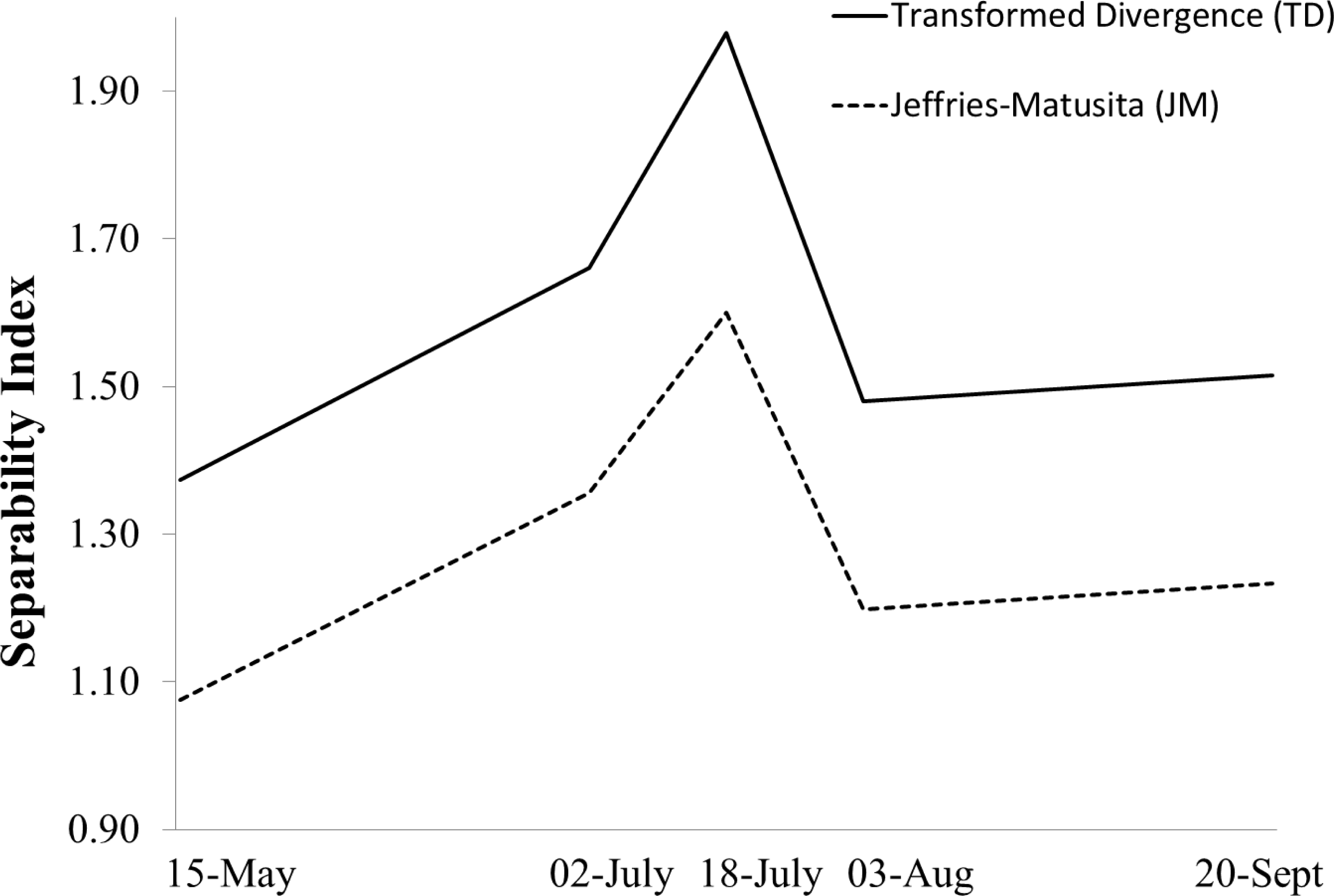
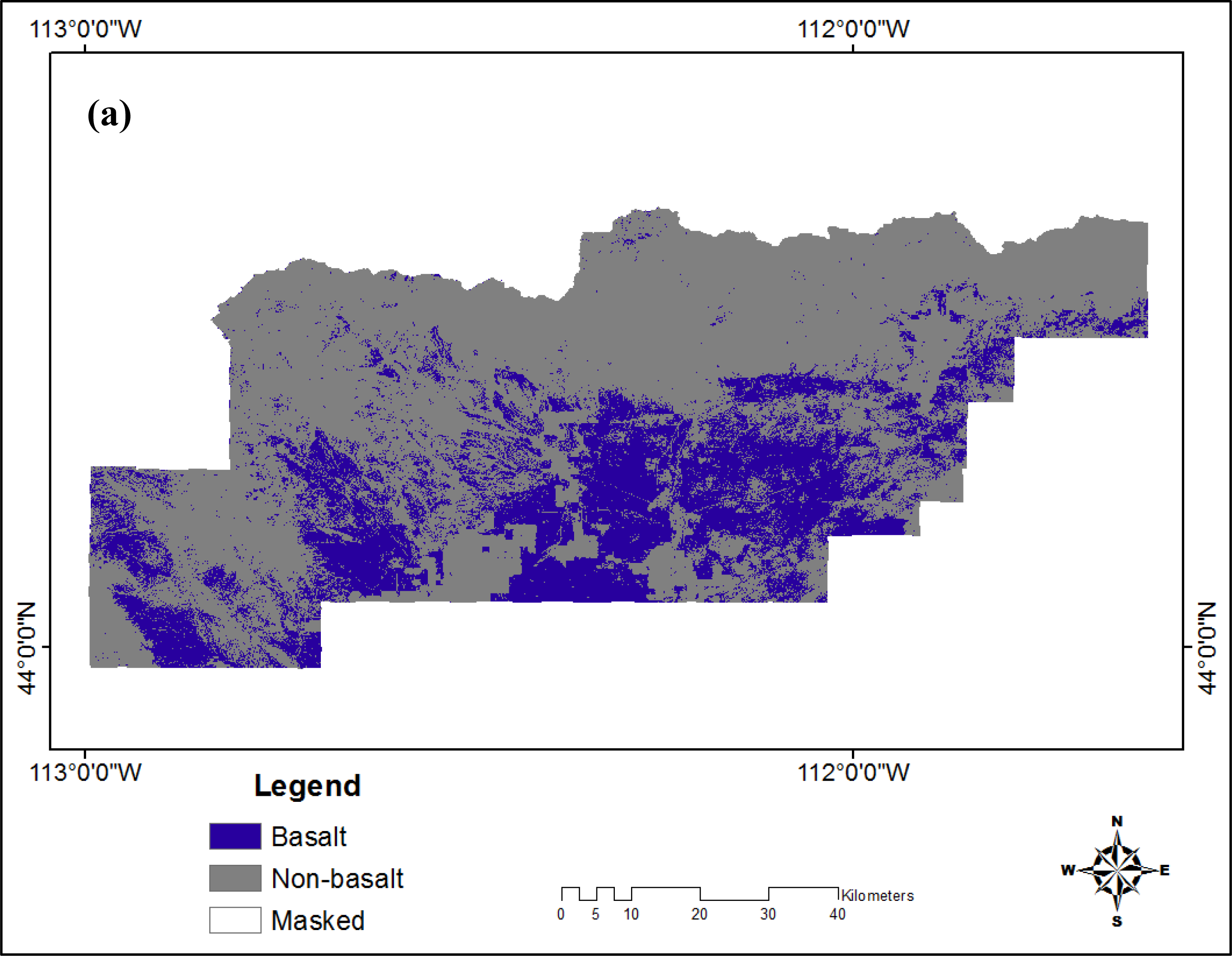
3.1. RCM Classifications

Classification results using RCM and the SAM method indicate that, on average, slightly greater accuracies are achieved using 18 July, rather than other single-date collections or the multitemporal stack (

Table 1. A comparison of average producer’s, user’s and overall accuracy results obtained from the Robust Classification Method (RCM) using the Spectral Angle Mapper (SAM) classification method to detect basalt outcrops.

	Basalt Average (User’s|Producer’s)	Non-Basalt Average (User’s|Producer’s)	Avg. Overall Average Accuracy	Average Kappa Coefficient
15 May 2007 (13 bands)	66.77%|63.50%	44.97%|48.31%	57.70%	0.12
2 July 2007 (13 bands)	66.01%|58.82%	45.45%|51.38%	55.98%	0.10
18 July 2007 (13 bands)	66.28%|68.65%	49.32%|51.03%	60.45%	0.12
3 August 2007 (13 bands)	62.40%|57.03%	39.55%|44.72%	52.32%	0.02
20 September 2007 (13 bands)	59.08%|53.87%	34.89%|59.02%	48.58%	−0.06
Multitemporal Stack (65 bands)	66.12%|67.80%	46.74%|43.89%	58.67%	0.12

). The improved results from 18 July are likely influenced by the separability described above, with vegetation senesced and basalt cover maximized. User’s and producer’s accuracies were consistently close in value, which indicates a tendency to neither over-predict nor under-predict; however, low kappa coefficients suggest that the classifications could be performing only slightly better than classification results generated by chance. Overall, basalt classification accuracies were higher than non-basalt classification accuracies and may be related to the number of basalt ROI pixels (n = 68) compared to the number of non-basalt ROI pixels (n = 41). The majority classification map that was generated by the RCM classifications (Figure 4a) indicated the presence of basalt across areas of known lava fields in the southeastern portion of Clark County; however, occurrences outside of the general area of lava flow may be false positives. Many of these occurrences coincide with areas of low uncertainty (50%–70% majority), which could be improved through additional sampling efforts. Classification uncertainty, as measured by the percent of repetitions for which individual pixels were assigned to the majority class (Figure 4b), was lowest across irrigated land, riparian areas and forested hillslopes. Classification uncertainty tended to be highest in xeric areas and areas of bright soil reflectance, including dirt roads.

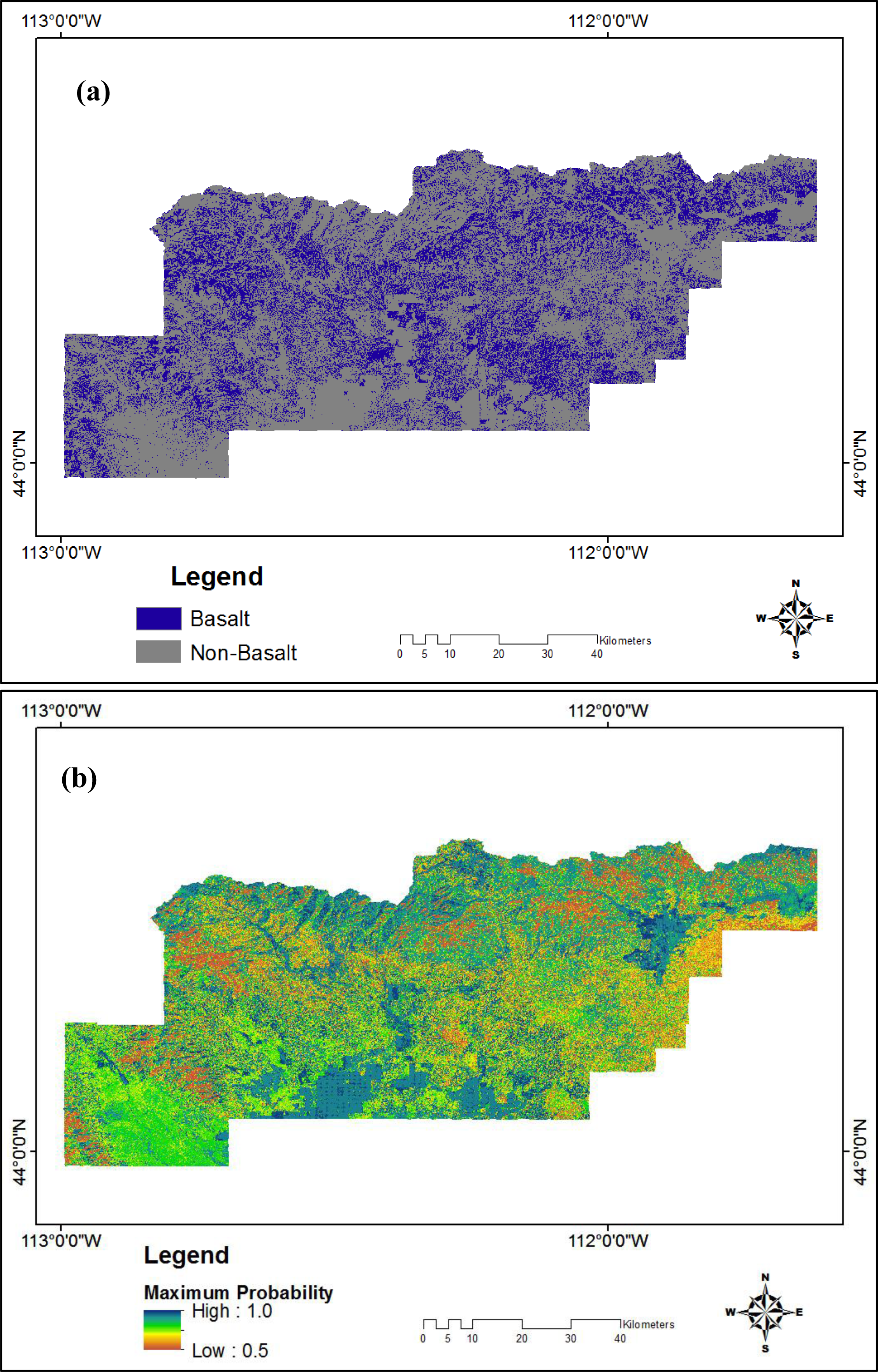
3.2. RF Classifications

Random Forest results indicated that the multi-temporal stack performed better than any individual scene date when considering overall classification rate and receiver operator characteristic (ROC) area under curve (AUC) statistics (

Table 2. A comparison of classification accuracy results obtained using Random Forest (RF) to detect basalt outcrops. ROC, receiver operator characteristic; OOB, out-of-bag; NDVI, Normalized Difference Vegetation Index.

Landsat Data	No. of Bands	Average Log Likelihood	ROC (Area Under Curve)	Non-Basalt Prediction (OOB) Success	Basalt Prediction (OOB) Success	Classification Rate (Overall)	Best Variables
5 time series (5/15/2007 to 9/20/2007)	65	0.57	0.79	82.93%	61.76%	72.35%	Greenness (7/2/2007) Band 4 (0.83 μm 7/18/2007) Greenness (9/20/2007) NDVI
15 May 2007	13	0.76	0.63	75.61%	50.00%	62.81%	Greenness Brightness Band 7 (2.215 μm)
2 July 2007	13	0.65	0.73	85.37%	55.88%	70.63%	Greenness Band 4 (0.83 μm) Wetness NDVI
18 July 2007	13	0.66	0.72	80.49%	61.76%	71.13%	Band 4 (0.83 μm) Greenness Band 1 (0.485 μm)
3 August 2007	13	0.69	0.66	73.17%	41.18%	57.18%	Wetness Band 4 (0.83 μm) Greenness Band Ratio 4:7 (0.83 μm: 2.215 μm)
20 September 2007	13	0.74	0.64	70.73%	54.41%	62.57%	Greenness Band 4 (0.83 μm) Band Ratio 4:7 (0.83 μm: 2.215 μm)

). The three most important variables in predicting basalt and non-basalt locations in the multitemporal stack were TC greenness values from the 2 July and the 20 September scenes and Band 4 from the 18 July scene. The TC greenness index was also consistently identified as an important variable for all five single-date classifications. Even though the TC greenness index is sensitive to topography [46], it is known to be less sensitive to soil type and moisture [47], thus providing an important measure for separating vegetation from basalt rocks in a study area with relatively flat terrain. Of interest also is the identification of Band 1 as an important variable in the July 18 classification, which performed as well as the multitemporal stack in predicting basalt. The spectral information from Band 1 may have emphasized the basalt weathering and/or mineralogy during a time of vegetation senescence. Contrary to our expectations, the thermal band did not perform well and was not one of the top ten best variables in any of the single date or multitemporal stack imagery. This might be due to the scale (120 m) of the thermal band in Landsat (which was resampled to 30 m) being too coarse compared to the rock outcrop ROIs.

The best performing classification output (multitemporal stack) that was generated by the RF classifications (Figure 5a) indicated the presence of basalt across areas of known lava fields in the southeastern portion of Clark County; however, occurrences outside of the general area of lava flow may be false positives. Classification uncertainty, as measured by computing the maximum of the probability of class membership between basalt and non-basalt classes (Figure 4b), resulted in an evenly distributed range of values. Areas of lower uncertainty tended to coincide with irrigated lands and, to a lesser extent, with riparian areas and forested hillslopes. Classification uncertainty tended to be highest in areas influenced by shadow.

3.3. Comparative Results

For both the RCM and the RF approach, the highest basalt classification results were achieved using the 18 July scene (13 bands). The RCM approach resulted in a 68.65% producer’s accuracy and a 66.28% user’s accuracy. The RF approach resulted in a 61.76% rate of successful basalt prediction. The multitemporal stack performed equally as well as the 18 July scene in predicting basalt in the RF classification and generated the highest overall classification accuracy (72.35%). The OOB estimates of error generated by the RF classification, although not directly comparable to the user’s and producer’s accuracy rates generated in RCM, do suggest that RF classification did a better job overall at predicting non-basalt occurrences. The OOB estimates of non-basalt prediction success for RF classification ranged from 70.73% to 82.93%, while the non-basalt user’s and producer’s accuracies for RCM ranged from 34.89% to 46.74% and from 43.89% to 59.02%, respectively. The OOB estimates of successful basalt prediction using RF ranged from 41.18% to 61.76%, while the basalt user’s and producer’s accuracies for RCM ranged from 59.08% to 66.77% and from 53.87% to 68.65%, respectively. The RCM approach using the SAM method compares the spectral similarity by calculating the angle between the image spectra and the training endmember spectra, whereby smaller angles represent greater degrees of similarity. In contrast, the RF approach is decision-tree based and tends to perform better when a large number of predictor variables are included in the analysis. This could explain why the multitemporal stack performed best using RF, while the July 18 scenario performed best using the RCM. On the other hand, it should be noted that the greenness from July and the greenness from August in the multitemporal stack are not significantly correlated (r = 0.67, n. s. at 0.05). This example highlights the importance of using a multi-date stack to represent a range of spectral variability within the best predictor(s) (the greenness band in this case). For optimal RCM and RF classifications, uncertainty tended to be lowest in irrigated areas; however, the RCM uncertainty map included more extensive areas of low uncertainty that also encompassed forested hillslopes and riparian areas (Figures 4a and 5b). RCM uncertainty was sensitive to the influence of bright soil reflectance, while RF uncertainty was sensitive to the influence of shadows.

3.4. Limitations

Primary limitations for this study were related to field data collection, image acquisition dates, accuracy assessment methods and, to a lesser degree, georegistration errors. The time lag between the 2007 images and 2007–2008 field data collection left some speculation as to the validity of recorded field observations in relation to the imagery. The fractional presence of exposed basalt could be confounded by changes in vegetation and soil coverage between image acquisition and field data collection dates. In addition, the number of polygons collected within the project area was not balanced between basalt and vegetation; therefore, bias may have been introduced in the accuracy assessments and could have contributed to low producer’s accuracies. Selection of a specific map unit and a balanced collection of polygons within its boundary before image processing begins would provide more conclusive results. Another limitation associated with field data collection was a range of polygon sizes and composition. Uncertainty is expected to increase in cases where overlap between Landsat pixels and ground reference polygons was minimal; for example, in areas where small polygons were located on the boundary of two Landsat pixels. Uncertainty is also expected to increase in cases where basalt ground reference polygons cover small areas or where the percent coverage is relatively low. Georegistration errors in the terrain-corrected imagery were low (3.73 to 4.60 m), as were the co-registration errors (0.02 to 0.33 m), and errors from the GPS locations of ground truth data were estimated to be less than 1 m (Trimble Navigation Limited, Westminster, CO, USA). Because these errors were well within one image pixel (30 m), the application of buffers to the ground truth data to accommodate potential positioning errors were not used in this study. A topographic correction was not applied to the imagery; while there is large topographic relief in the northern portions of Clark County, the majority of the mapping occurred across elevation ranging less than 500 m. Regardless, a topographic correction could assist with normalizing the reflectance across dates, thus improving sensitivity to basalt.

3.5. Further Research

Continued studies should focus on methods to overcome the effects of mixed pixels and maximize class separation by accentuating the target and minimizing background components. Hybrid techniques that combine multiple methods, such as NDVI, supervised classification, spectral mixture analysis and image segmentation on multitemporal images have been found to effectively increase performance over traditional multispectral classification methods [48,49]. We suggest more selective band choices to create a multitemporal stack [42], stacking images acquired over multiple years and possibly coupling the Landsat data with information from LiDAR, InSAR or IFSAR to emphasize both spectral and textural features [8,9].

Considering the high percentage of lichen cover on basalt in the study area, methods to detect lichen should also be investigated as a means to indirectly detect basalt and rock outcrops in similar soilscapes. The spectral reflectance of rock growing lichens has been found to be unique to that of other surface types and land covers [50], and the spectral response changes with the availability of water F53 [51].

4. Conclusions

Our study demonstrates that Landsat imagery can detect the presence of basalt outcrops in western rangelands with an overall accuracy rate of 72.35% using RF classification using a multitemporal stack of Landsat images that included both surface reflectance values and derivatives, such as band ratios and indices (i.e., NDVI, TC greenness, wetness and brightness; Band 4 to Band 6 ratio). The highest overall classification accuracy generated from the RCM classifications (SAM method) was 60.45% and was influenced by relatively low non-basalt user’s and producers accuracies (50.06% to 50.80%). These basalt classifications represent a significant first step toward quantification and warrant continued research to obtain sub-pixel abundance values and resolve over-predictions of basalt caused by mixed pixels from vegetation, lichen and loess. We recommend that future studies investigate the variability of lichen spectral reflectance across space and time and under different soil moisture conditions using a field spectroradiometer to determine if spectral mixing techniques (e.g., [52]) are feasible at the 30-m pixel resolution with an added focus on lichen coverage estimated from hyperspectral sensors, such as Hyperion [53]. We also recommend developing and testing a multi-sensor approach that adds textural and height components, additional field data that are more coincident with remote sensing acquisitions and decision tree classification. With further development, remote sensing can be a useful tool to support soil survey efforts in the Western United States and other regions of the world with similar soilscapes.

References

1. Jarmer, T.; Hill, J.; Lavee, H.; Pariente, S. Mapping topsoil organic carbon in non-agricultural semi-arid and arid ecosystems of Israel. Photogramm. Eng. Remote Sens 2010, 76, 85–94. [Google Scholar]
2. Leverington, D.W.; Moon, W.M. Landsat-TM-based discrimination of lithological units associated with Purtuniq Ophiolite, Quebec, Canada. Remote Sens 2012, 4, 1208–1231. [Google Scholar]
3. Nield, S.J.; Boettinger, J.L.; Ramsey, R.D. Digitally mapping gypsic and natric soil areas using Landsat ETM data. Soil Sci. Soc. Am. J 2007, 71, 245–252. [Google Scholar]
4. Mshiu, E.E. Landsat remote sensing data as an alternative approach for geological mapping in Tanzania: A case study in the Rungwe volcanic province, South-Western Tanzania. Tanz. J. Sci 2011, 37, 26–36. [Google Scholar]
5. Frazier, B.E.; Cheng, Y. Remote sensing of soils in the eastern Palouse region with Landsat Thematic Mapper. Remote Sens. Environ 1989, 28, 317–325. [Google Scholar]
6. Harris, J.R.; Grunsky, E.C.; He, J.; Gorodetzky, D.; Brown, N. A robust, cross-validation classification method (RCM) for improved mapping accuracy and confidence metrics. Can. J. Remote Sens 2012, 38, 69–90. [Google Scholar]
7. Behnia, P.; Harris, J.R.; Rainbird, R.H.; Williamson, M.C.; Sheshpari, M. Remote predictive mapping of bedrock geology using image classification of Landsat and SPOT data, western Minto Inlier, Victoria Island, Northwester Territories, Canada. Int. J. Remote Sens 2012, 33, 6876–6903. [Google Scholar]
8. Gaber, A.; Koch, M.; El-Baz, F. Textural and compositional characterization of Wadi Feiran deposits, Sinai Peninsula, Egypt, using Radarsat-1, PALSAR, SRTM and ETM+ data. Remote Sens 2010, 2, 52–75. [Google Scholar]
9. Inzana, J.; Kusky, T.; Higgs, G.; Tucker, R. Supervised classifications of Landsat TM band ratio images and Landsat TM band ratio image with radar for geological interpretations of central Madagascar. J. Afr. Earth Sci 2003, 37, 59–72. [Google Scholar]
10. Sellers, P.J. Canopy reflectance, photosynthesis and transpiration. Int. J. Remote Sens 1985, 6, 1335–1372. [Google Scholar]
11. Loizzo, R.; Sylos Labini, G.; Pappalepore, M.; Pieri, P.; Pasquariello, G.; Antoninetti, M. Multitemporal and Multisensory Signatures Evaluation for Lithologic Classification. Proceedings of International Geoscience and Remote Sensing Symposium (IGARSS ’95), Quantitative Remote Sensing for Science and Applications, Firenze, Italy, 10–14 July 1995; 3, pp. 2509–2211.
12. Idawo, C.; Laneve, G. Hyperspectral Analysis of Multispectral ETM+ Data: SMA Using Spectral Field Measurements in Mapping of Emergent Macrophytes. Proceedings of the IEEE Geoscience and Remote Sensing Symposium (IGARSS 2004), Anchorage, AK, USA, 20–24 September 2004; 1, p. 249.
13. Van der Meer, F.; de Jong, S.M. Improving the results of spectral unmixing of Landsat Thematic Mapper imagery by enhancing the orthogonality of end-members. Int. J. Remote Sens 2000, 21, 2781–2797. [Google Scholar]
14. Zhang, X.; Pazner, M.; Duke, N. Lithologic and mineral information extraction for gold exploration using ASTER data in the south Chocolate Mountains (California). ISPRS J. Photogramm. Remote Sens 2007, 62, 271–282. [Google Scholar]
15. De Asis, A.M.; Omasa, K.; Oki, K.; Shimizu, Y. Accuracy and applicability of linear spectral unmixing in delineating potential erosion areas in tropical watersheds. Int. J. Remote Sens 2008, 29, 4151–4171. [Google Scholar]
16. Gill, T.K.; Phinn, S.R. Improvements to ASTER-derived fractional estimates of bare ground in a Savanna Rangeland. IEEE Trans. Geosci. Remote Sens 2009, 47, 662–670. [Google Scholar]
17. Leverington, D.W. Discrimination of sedimentary lithologies using Hyperion and Landsat Thematic Mapper data: A case study at Melville Island, Canadian High Arctic. Int. J. Remote Sens 2010, 31, 233–260. [Google Scholar]
18. Moore, C.; Hoffman, G.; Glenn, N. Quantifying basalt rock outcrops in NRCS soil map units using Landsat 5 TM data. Soil Surv. Horizons 2007, 48, 59–62. [Google Scholar]
19. Southworth, J. An assessment of Landsat TM band 6 thermal data for analysing land cover in tropical dry forest regions. Int. J. Remote Sens 2004, 25, 689–706. [Google Scholar]
20. Knick, S.T.; Rotenberry, J.T.; Zarriello, T.J. Supervised classification of Landsat Thematic Mapper imagery in a semi-arid rangeland by nonparametric discriminant analysis. Photogramm. Eng. Remote Sens 1997, 63, 79–86. [Google Scholar]
21. Martínez-Montoya, J.F.; Herrero, J.; Casterad, M.A. Mapping categories of gypseous lands in Mexico and Spain using Landsat imagery. J. Arid Environ 2010, 74, 978–986. [Google Scholar]
22. Singh, N.; Glenn, N.F. Multitemporal spectral analysis for cheatgrass (Bromus tectorum) classification. Int. J. Remote Sens 2009, 30, 3441–3462. [Google Scholar]
23. Key, T.; Warner, T.A.; McGraw, J.B.; Fajvan, M.A. A comparison of multispectral and multitemporal information in high spatial resolution imagery for classification of individual tree species in a temperate hardwood forest. Remote Sens. Environ 2001, 75, 100–112. [Google Scholar]
24. Song, C.; Woodcock, C.E. Monitoring forest succession with multitemporal Landsat images: Factors of uncertainty. IEEE Trans. Geosci. Remote Sens 2003, 41, 2557–2567. [Google Scholar]
25. Pal, M.; Mather, P.M. Support vector machines for classification in remote sensing. Int. J. Remote Sens 2005, 26, 1007–1011. [Google Scholar]
26. Ham, C.; Chen, Y.; Crawford, M.M.; Ghosh, J. Investigation of the random forest framework for classification of hyperspectral data. IEEE Trans. Geosci. Remote Sens 2005, 43, 492–501. [Google Scholar]
27. Hughes, G.F. On the mean accuracy of statistical pattern recognizers. IEEE Trans. Inf. Theory 1968, 14, 55–63. [Google Scholar]
28. Raudys, S.J.; Jain, A.K. Small sample size effects in statistical pattern recognition: Recommendations for practitioners. IEEE Trans. Pattern Anal. Mach. Intell 1991, 13, 252–264. [Google Scholar]
29. Breiman, L. Random forests. Mach. Learn 2001, 45, 5–32. [Google Scholar]
30. Pal, M. Random forest classifier for remote sensing classification. Int. J. Remote Sens 2005, 26, 217–222. [Google Scholar]
31. Hudak, H.T.; Crookston, N.L.; Evans, J.S.; Hall, D.E.; Falkowski, M.J. Nearest neighbor imputation of species-level, plot scale forest structure attributes from LiDAR data. Remote Sens. Environ 2008, 112, 2232–2245. [Google Scholar]
32. Digital Atlas of Idaho. Available online: http://imnh.isu.edu/digitalatlas/ (accessed on 10 January 2012).
33. US Department of Agriculture, Natural Resources Conservation Service. National Soil Survey Handbook (NSSH); Natural Resources Conservation Service, National Soil Survey Center: Lincoln, NE, USA, 2006. [Google Scholar]
34. Hawth’s Analysis Tools for ArcGIS. Available online: http://www.spatialecology.com/htools/tooldesc.php (accessed on 10 January 2012).
35. US Department of Agriculture, Natural Resources Conservation Service. Field Book for Describing and Sampling Soils, ed. 2.0; Schoeneberger, P.J., Wysocki, D.A., Benham, E.C., Broderson, W.D., Eds.; Natural Resources Conservation Service, National Soil Survey Center: Lincoln, NE, USA, 2002. [Google Scholar]
36. ITT Visual Information Solutions. Environment for Visualizing Images (ENVI) 4.8; ITT Visual Information Solutions: Boulder, CO, USA, 2007. [Google Scholar]
37. Environmental Systems Research Institute (ESRI). ArcGIS 10.1; ESRI: Redlands, CA, USA, 2005. [Google Scholar]
38. Adler-Golden, S.M.; Matthew, M.W.; Bernstein, L.S.; Levine, R.Y.; Berk, A.; Richtsmeier, S.C.; Acharya, P.K.; Anderson, G.P.; Felde, G.; Gardner, J.; et al. Atmospheric correction for short-wave spectral imagery based on MODTRAN4. Proc. SPIE 1999, 3753, 61–69. [Google Scholar]
39. Coll, C.; Galve, J.M.; Sánchez, J.M.; Caselles, V. Validation of Landsat-7/ETM+ thermal-band calibration and atmospheric correction with ground-based measurements. IEEE Trans. Geosci. Remote Sens 2010, 48, 547–555. [Google Scholar]
40. Crist, E.P.; Cicone, R.C. Application of the tasseled cap concept to simulated thematic mapper data. Photogramm. Eng. Remote Sens 1984, 50, 343–352. [Google Scholar]
41. Richards, J.A.; Jia, X. Remote Sensing Digital Image Analysis; Springer-Verlag: Berlin, Germany, 2006. [Google Scholar]
42. Liu, Q.J.; Takamura, T.; Takeuchi, N.; Shoa, G. Mapping of boreal vegetation of a temperate mountain in China by multi-temporal Landsat TM imagery. Int. J. Remote Sens 2002, 23, 3385–3405. [Google Scholar]
43. Kuemmerle, T.; Roder, A.; Hill, J. Separating grassland shrub and vegetation by multidate pixel-adaptive spectral mixture analysis. Int. J. Remote Sens 2006, 27, 3251–3271. [Google Scholar]
44. Wang, J.; Lang, P. Detection of cypress canopies in the florida panhandle using subpixel analysis and GIS. Remote Sens 2009, 1, 1028–1042. [Google Scholar]
45. Breiman, L.; Friedman, J.H.; Olshen, R.A.; Stone, C.J. Classification and Regression Trees; Wadsworth, Inc: Pacific Grave, CA, USA, 1984. [Google Scholar]
46. Cohen, W.B.; Spies, T.A. Estimating structural attributes of Douglas-Fir/Western Hemlock forest stands from Landsat and SPOT imagery. Remote Sens. Environ 1992, 41, 1–17. [Google Scholar]
47. Todd, S.W.; Hoffer, R.M.; Milchunas, D.G. Biomass estimation on grazed and ungrazed rangelands using spectral indices. Int. J. Remote Sens 1998, 19, 427–438. [Google Scholar]
48. Hepinstall-Cymerman, J.; Coe, S.; Alberti, M. Using urban landscape trajectories to develop a multi-temporal land cover database to support ecological modeling. Remote Sens 2009, 1, 1353–1379. [Google Scholar]
49. Powell, R.L.; Roberts, D.A.; Dennison, P.E.; Hess, L.L. Sub-pixel mapping of urban land cover using multiple endmember spectral mixture analysis: Manaus, Brazil. Remote Sens. Environ 2007, 106, 253–267. [Google Scholar]
50. Van der Veen, C.J.; Csatho, B.M. Spectral characteristics of Greenland lichens. Geographie Physique et Quaternaire 2005, 59, 63–73. [Google Scholar]
51. Karnieli, A.; Gabai, A.; Ichoku, C.; Zaady, E.; Shachak, M. Temporal dynamics of soil and vegetation spectral responses in a semi-arid environment. Int. J. Remote Sens 1996, 23, 4073–4078. [Google Scholar]
52. Mitchell, J.; Glenn, N. Subpixel abundance estimates in mixture-tuned matched filtering classifications of leafy spurge (Euphorbia esula L.). Int. J. Remote Sens 2009, 30, 6099–6119. [Google Scholar]
53. Huemmrich, K.F.; Gamon, J.A.; Tweedie, C.E.; Campbell, P.K.E.; Landis, D.R.; Middleton, E.M. Arctic tundra vegetation functional types based on photosynthetic physiology and optical properties. IEEE J. Sel. Top. Appl. Earth Obs. Remote Sens 2013, 6, 265–275. [Google Scholar]
Figure 1. The basalt mapping study area and field sampling locations in Clark County, ID, USA.
Remotesensing 05 04857f1
Figure 2. The extent and amount of exposed basalt rock outcrops is highly variable on the Eastern Snake River Plain, with most outcrops partially obscured by grasses and sagebrush. (a) Pressure ridges. (b) Columnar vesicular basalt.
Remotesensing 05 04857f2
Figure 3. Measures of separability obtained from individual scene dates in 2007 (15 May, 2 July, 18 July, 3 August and 20 September) between pairs of basalt and non-basalt reference data. Values greater than 1.9 are considered to have good separability for classification.
Remotesensing 05 04857f3
Figure 4. Basalt mapping results obtained from 18 July Landsat scene using the Robust Classification Method (RCM) and the Spectral Angle Mapper (SAM) method, in Clark County, ID, USA. Average overall classification accuracy is 60.45%. (a) A classification uncertainty map was also generated by calculating where the percent majority is the percent of repetitions (60) that resulted in the pixel being assigned to the majority class. (b) A high percent majority value equates to low uncertainty.
Remotesensing 05 04857f4aRemotesensing 05 04857f4b
Figure 5. (a) Basalt mapping results obtained from the multitemporal Landsat scene using the Random Forest (RF) method, in Clark County, ID, USA. The overall classification rate is 72.35%. (b) A classification uncertainty map was also generated by computing the maximum of the probability of class membership between basalt and non-basalt classes. A high probability value equates to low uncertainty.
Remotesensing 05 04857f5