Orthogonal Equations of Multi-Spectral Satellite Imagery for the Identification of Un-Excavated Archaeological Sites

Abstract

This paper aims to introduce new linear orthogonal equations for different satellite data derived from QuickBird; IKONOS; WorldView-2; GeoEye-1, ASTER; Landsat 4 TM and Landsat 7 ETM+ sensors, in order to enhance the exposure of crop marks. The latest are of significant value for the detection of buried archaeological features using remote sensing techniques. The proposed transformations, re-projects the initial VNIR bands of the satellite image, into a new 3D coordinate system where the first component is the so called “crop mark”, the second component “vegetation” and the third component “soil”. For the purpose of this study, a large ground spectral signature database has been explored and analyzed separately for each different satellite image. The narrow band reflectance has been re-calculated using the Relative Spectral Response filters of each sensor, and then a PCA analysis was carried out. Subsequently, the first three PCA components were rotated in order to enhance the detection of crop marks. Finally, all proposed transformations have been successfully evaluated in different existing archaeological sites and some interesting crop marks have been exposed.

1. Introduction

Detection of buried archaeological features using medium or high resolution satellite imagery is a well-established procedure in archeological research [1–8]. Buried structures may be identified mainly by image interpretation of crop marks [9–11] or using semi-automatic techniques [12,13]. These marks are formed in areas where vegetation overlays near-surface archaeological remains. This is due to the fact that archaeological features tend to retain different percentages of soil moisture compared to the rest of the crops of an area. In this way, spectral differences of crops, especially in the Near Infrared (NIR ) part of spectrum, may be recorded. Depending on the type of the buried archaeological features, crop vigour may be enhanced or reduced [14].

Crop marks are very common in geoarchaeology and initially studied using aerial photographs. As [15] report in their study, crop marks (positive or negative) are caused as an indirect effect of buried structures. Positive crop marks may appear in areas where subsurface trenches exist since the cover material retains dampness, resulting in the plants growing more densely and maturing later than those in neighbouring sites. In contrary, negative crop marks appear in areas where the plants grow over the buried remains of human structures, where the soil is poor in nitrates, with no dampness, and therefore it cannot help plant growth [11].

Though, if vegetation grows above buried ditches or moat, then the crop growth is likely to be enhanced. This is due to the topsoil which holds more moisture than in the surrounding context (especially during periods when water stress develops). This phenomenon can be recorded from any airborne and spaceborne platform and is referred to as a positive crop mark [4,10,11]. However, in cases where there is not enough moisture in the retentive soil and there is lack of available water for evapotransporation (e.g., vegetation grown above building remains or compacted ground), the developed marks are characterized as negative crop marks. These are less common than the positive ones [4,10,11]. Comparing the two different kinds of marks, the positives are normally taller with darker green and healthy foliage than the negative crop marks. On the other hand, the negative crop marks tend to be paler green with lighter coloured appearance when monitored from the air [10,11].

The use of remote sensing data for supporting archaeological research has been increased in the last decade due to the higher spatial resolution capabilities of the new satellite sensors [16,17]. Many scholars have been able to reveal archaeological remains beneath ground surface, using a variety of existing algorithms with different rate of success [18–22]. However, the development of new or the modification of existing algorithms for supporting archaeological research is still very limited. This is due to the fact that the formation of crop marks is a very complicated phenomenon [14,23]. Several climatic and soil parameters should be taken into consideration when examining crop marks. In addition, the formation of crop marks is a dynamic phenomenon and therefore spectral characteristics of crops may vary during the different phenological stages [21]. Indeed several parameters should be taken into consideration, such as the characteristics of the buried features, the burial depth of them, soil characteristics, climatic and environmental parameters, cultivation techniques, etc. [15,21–23]. Furthermore, moisture availability and the availability of dissolved nutrients to the crops (at crucial growing times and periods for the plant) are also important parameters that need to be considered.

This paper aims to address this problem and to introduce new linear orthogonal equations for the enhancement of crop marks, for several existing medium and high resolution satellite sensors. These linear transformations are based on the physical characteristics of crop marks, vegetation and soil. The algorithms are based on the work of Kauth-Thomas [24], also known as Tasseled Cap transformation (K-T algorithm), in order to detect vegetation in satellite data. K-T algorithm is a widely used metric capable of capturing scene characteristics in related coordinate directions in a defined feature space [25]. This transformation reduces the satellite reflectance bands to three orthogonal indices called brightness, greenness and wetness [26]. The main advantage of the K-T transformation compared to other existing algorithms is the fact that the coefficients of this linear transformation are calculated in order to enhance specific characteristics of the satellite image (i.e., vegetation). However, since new sensors are deployed, the wavelengths used to define each of the spectral bands depend on the relative spectral response (RSR) filters of the sensor for each particular bandwidth. Therefore, the nature of the tasseled-cap space is similar for each sensor, yet refinements of the T-C space coefficients must be investigated for each sensor [25]. Several researchers [27–30] have been able to define the new linear coefficients of the T-C algorithm for a variety of sensors using satellite image data. Nevertheless, the methodology followed can be problematic since pixels selected in satellite data (for the basis vector) should be at first radiometric and atmospheric corrected. Indeed, as [31] stated, total relative radiometric uncertainties of calibration are within 5% for satellite sensors. Moreover, errors occurred by atmospheric effects in satellite data influence the quality of the information extracted from remote measurements, such as vegetation indices [32,33]. These effects can increase the uncertainty by up to 10%, depending on the spectral band [34]. In addition, as [35] have shown, a mean difference of 18% of the NDVI algorithm between the atmospheric and non-atmospheric corrected satellite data can be recorded. Moreover, the sample taken for the formation of the basis vectors, from the satellite data, should be representative and the pixels should be not mixed, in order to avoid any noise and errors.

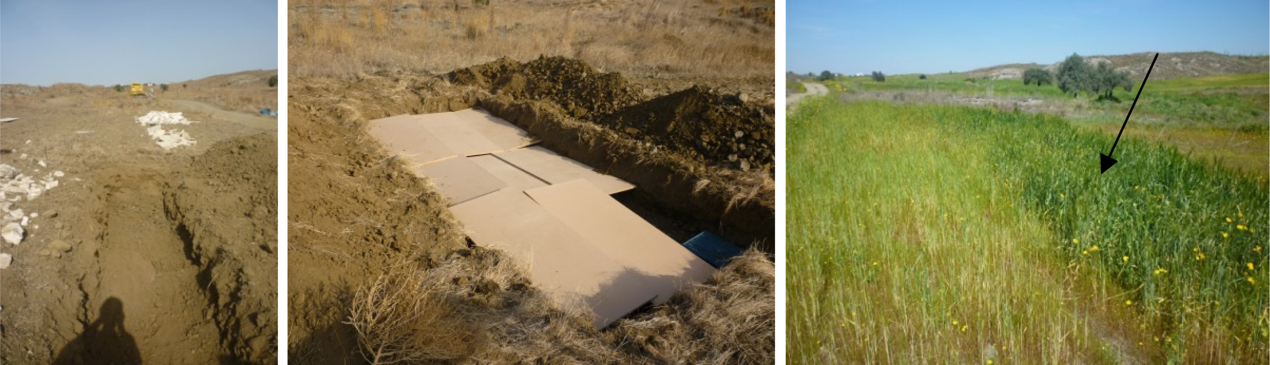
In order to overcome such limitations and to develop specific linear transformations for the enhancement of crop marks, vegetation and soil using satellite images, the authors have followed an alternative methodology based on simulated data taken from ground spectroradiometer. Systematic spectroradiometric campaigns were organized into a test field to record ground data during the whole phenological cycle of the crops. In this way, the dynamic nature of formation of crop marks was also observed, and pure reflectance values from crop marks, vegetation and bare soil were acquired.

2. Methodology and Resources

2.1. Case Studies: Controlled Field and Archaeological Sites

An extensive controlled archaeological test field was created at Alampra village located in central Cyprus (see [22,36]). The aim of this test field was to simulate archaeological environment for detecting architectural remains buried under ground soil. This test field was designed and developed in-situ, in order to systematically acquire ground spectral signatures of crops overlaying near-surface architectural remains. For the aims of this study, two 5 m × 5 m squares (“replicas”) were used to simulate the presence of swallow depth buried remains. In these squares, tombs were simulated by entrapment of air. Then, the test site was cultivated with crops according to the traditional methods of the area during the period of 2011–2012 (Figure 1). During this period, ground spectroradiometric data were systematically acquired.

The results from the field campaigns at the Alampra site were analyzed and linear coefficients for the enhancement of crop marks were calculated for several broadband satellite sensors. These new transformations were then evaluated to several existing archaeological sites of the eastern part of the Mediterranean region: Nea Paphos, ancient Elis and ancient Megalopolis as well to Neolithic tells in the region of Thessaly (see Figure 2).

2.2. Ground Spectroradiometric Measurements

Field spectroradiometers are used to provide calibrated and accurate reflectance measurements since these instruments are often accompanied by a calibrated Lambertian surface (spectralon panel). In cases where “single-beam” measurements are recorded, the measurements between the calibrated panel and the target (i.e., vegetation) should be taken in a short time (≈2 min). During this time interval the radiation is actually unchanged [37]. The radiation may be also affected by the zenith angle of the sun and the coordinates of the area of interest [38].

More than 16 field campaigns were organized in order to collect ground spectroradiometric data from the controlled field of Alampra. In each campaign, several ground spectroradiometric measurements were taken over the simulated “archaeological” and “non-archaeological” area (healthy site). For this purpose, a calibrated GER 1500 handheld spectroradiometer was used. GER 1500 has the ability to record electromagnetic radiation from visible to NIR spectrum (350–1,050 nm) using 512 different channels, with a range of ∼1.5 nm. Moreover, a Lambertian spectralon panel was also used in order to measure the incoming solar radiation and calibrate all the measurements taken over the crops. The field of view (FOV) of the instrument was set to 4 degrees (≈0.02 m² from a height of 1.2 m). At first the incoming radiance was calculated based on the reference measurement at the spectralon panel, while the following measurements were taken over the area of interest (either the archaeological or non-archaeological area). More than 1,700 ground spectral signatures were collected from crop marks, vegetation and soil.

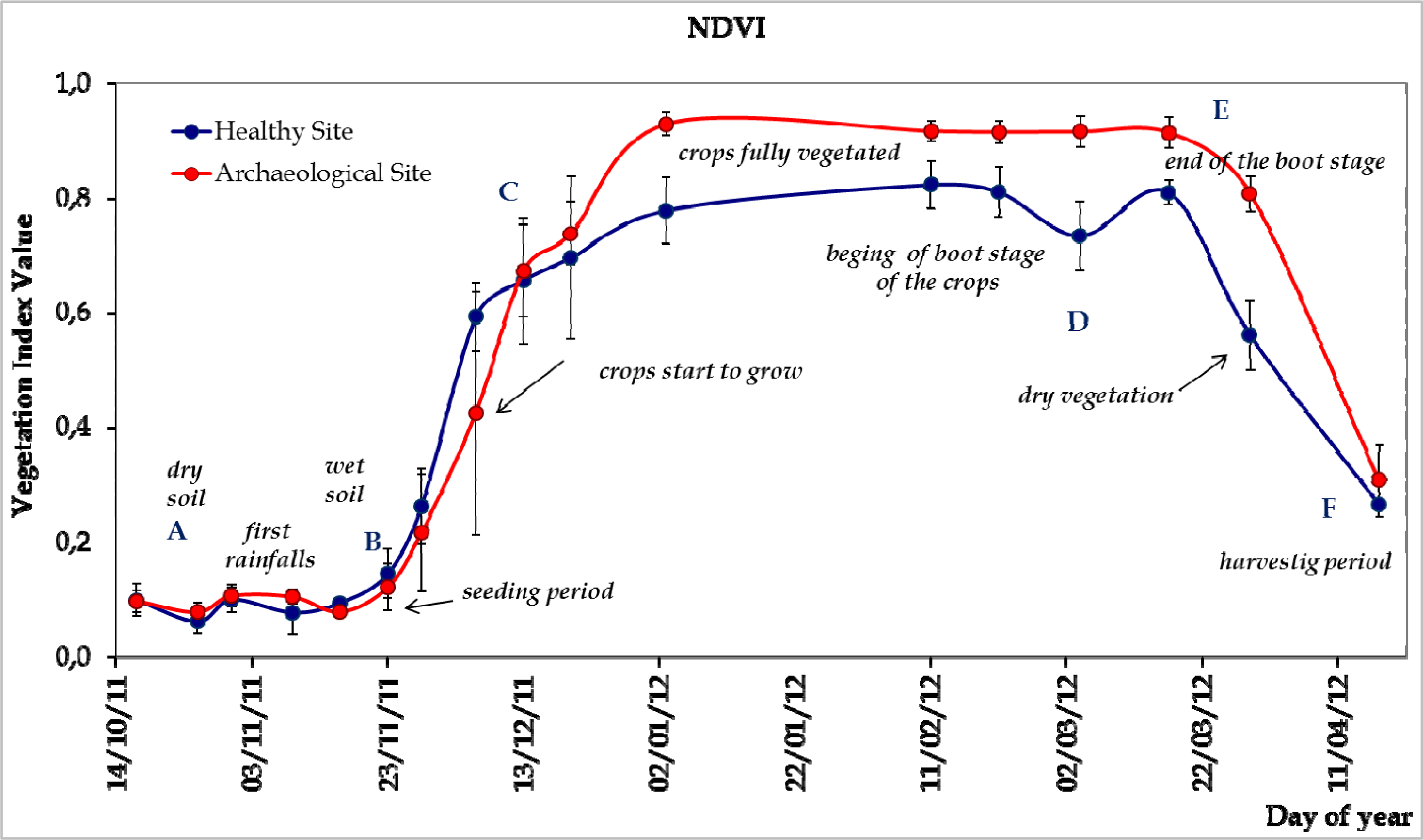
During these fields campaigns a complete phenological cycle of crops was observed. Characteristics points from the phenological cycle are marked in Figure 3 (Points A–F) while natural phenomena which can be observed in the field are also shown (in italics). As it is shown in Figure 3, Point A corresponds to dry soil, just before the first winter rainfalls. Wet soil, is shown in Point B and during the following period crops start to grow (Points B,C). During this period the crops are not fully vegetated and therefore crops do not cover the area of interest (i.e., soil background can be seen). After this short period the crops are fully vegetated (Points C–E). Point D shows the beginning of the boot stage of the crops until the end of the boot stage (Point E). Afterwards, the crops begin to dry (Point E to Point F) until the harvesting period (after Point F).The length of each period can be shorten or lengthen according to the type of crop cultivated, the soil characteristics and the climatic parameters [21]. As it was found from previous studies of the authors [21], during the boot stage of the crops the detection of crop marks is maximized.

2.3. Satellite Wavelengths

Several existing high and medium resolution satellite data have been evaluated for the purpose of this study. Specifically, the GeoEye-1; ASTER; IKONOS; Landsat 7 ETM+; Landsat 4 TM; QuickBird as well as WorldView-2 imagery were assessed for their capabilities to detect crops marks. As it was mentioned earlier, the linear coefficients for each dataset were calculated separately since each sensor has a different RSR filter and different spectral range of each particular bandwidth (from visible to the NIR part of the spectrum).

Table 1. Spectral characteristics of the satellite data used for the aims of this study in the Visible-Near Infrared (VNIR) part of the spectrum.

Satellite Sensor	Blue Band (nm)	Green Band (nm)	Red Band (nm)	VNIR Band (nm)	Spatial Resolution
GeoEye-1	450–520	520–600	625–695	760–900	1.65 m
ASTER	-	520–600	630–690	760–860	15 m
IKONOS	445–516	506–595	632–698	757–853	4 m
Landsat 7 ETM+	450–515	525–605	630–690	750–900	30 m
Landsat 4 TM	450–520	520–600	630–690	760–900	30 m
QuickBird	450–520	520–600	630–690	760–900	2.4 m

Table 1. Spectral characteristics of the satellite data used for the aims of this study in the Visible-Near Infrared (VNIR) part of the spectrum.

	Costal Band (nm)	Blue Band (nm)	Green Band (nm)	Yellow Band (nm)	Red Band (nm)	Red Edge Band (nm)	Near IR1 Band (nm)	Spatial Resolution
WorldView-2	400–450	450–510	510–580	585–625	630–690	705–745	770–895	0.50 m

presents the spectral range for each sensor used in this study. As it is demonstrated, spectral characteristics for each sensor can be different for the same spectral band, and therefore, spectral differences are expected. These variances are estimated to be 1%–8% for some of these sensors [17].

The sensors selected have been widely used for archaeological applications. High resolution satellite images from GeoEye-1, QuickBird, WorldView-2 as well as IKONOS are systematically used for supporting archaeological research [39–41]. In addition, Landsat images and ASTER are often used due to their historic value and low cost [42].

Ground narrowband measurements were simulated for the above satellite sensors systems using the appropriate RSR filters. The RSR filters for each sensor were obtained from different sources: published data, (WorldView-2); the operator’s websites (GeoEye-1, IKONOS, Landsat 7 ETM+, Landsat 4 TM, ASTER) and personal communication (QuickBird).

The spectral band responses ρ for each sensor were simulated by integrating the measured radiances (at the top of the canopy) for each target, with the spectral response curve applied as a weighting function, i.e.,

$$\rho =\frac{{\int }_{\lambda 1}^{\lambda 2}w(\lambda )\hspace{0.17em}R(\lambda )d\lambda }{{\int }_{\lambda 1}^{\lambda 2}w(\lambda )I(\lambda )d(\lambda )}$$

(1)

where R is the measured reflected radiation at the top of the canopy as a function of wavelength λ, w is the relative response of the broadband sensor and I is the corresponding incident radiance measured on an ideal reference panel. The actual reference panel measurement I is corrected to the ideal (100% reflectance) by dividing the measured value by its true reflectance ρ_ref.

$$\rho =\frac{{\int }_{\lambda 1}^{\lambda 2}w(\lambda )R(\lambda )d\lambda }{{\int }_{\lambda 1}^{\lambda 2}w(\lambda )I(\lambda )d\lambda }$$

(2)

Equation (1) presents the integrated band reflectance, as if measured by an actual broadband satellite sensor at the same time as the ground narrowband spectroradiometric measurements. As Steven et al. [43] argued, there is some variation in the band reflectance with solar angle and atmospheric conditions, which affect the spectral balance of the irradiance within the band. However, in practice, the spectral balance of solar irradiation is conservative once solar elevation exceeds 10° and therefore errors involved in applying this approach is minimal [44].

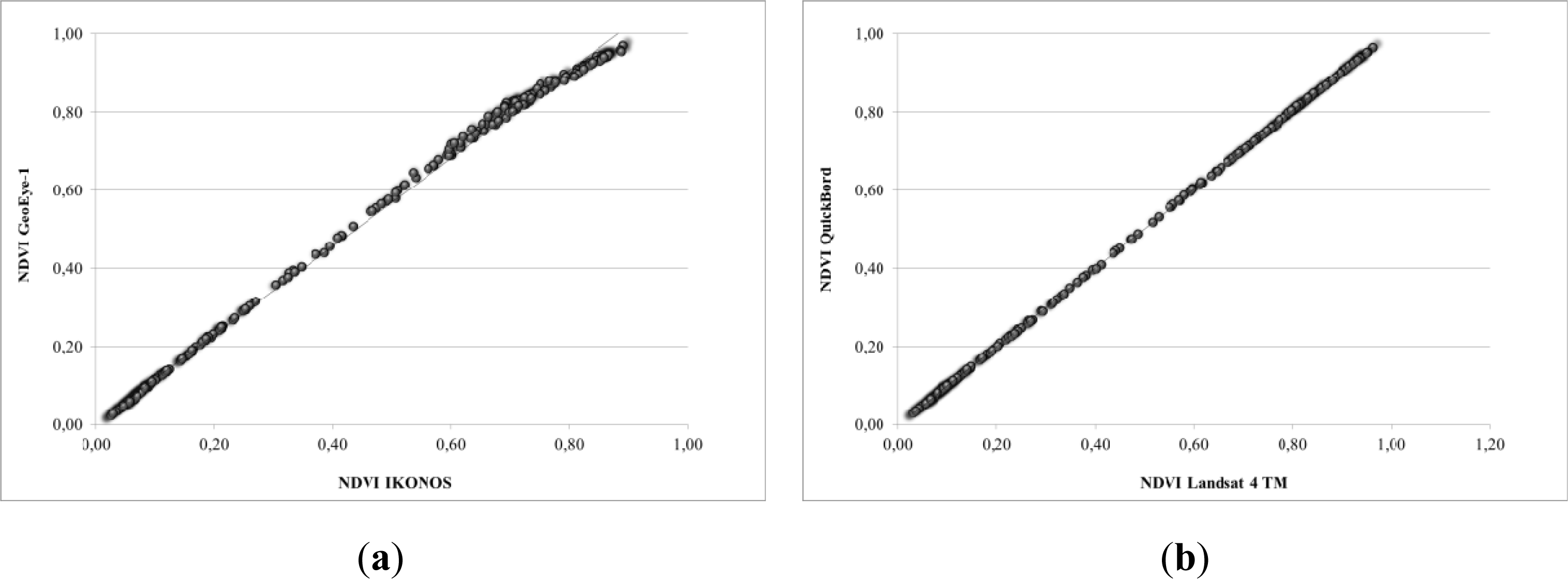
As it is shown in Figure 4, a strong linear relationship of the NDVI profile between all satellites sensors exist based on the whole dataset. However, differences in the distribution of the NDVI values is also observed, which indicates the impact of the RSR filters on the simulated data and the difference spectral capabilities of each sensor using the same data.

2.4. Calculation of n-Space Coefficients

For the calculation of the n-space coefficients for all satellite sensors used in this study, the following methodology was followed, separately for each sensor:

• Step 1: At first all narrowband spectral signatures were re-calculated based on the appropriate RSR filters of each sensor using Equations (1) and (2). This was necessary in order to simulate the ground data to at-satellite broadband reflectance. As [25] argue, this step is necessary since the shape of transformation is dependent on the spectral response of the sensors. Therefore, sensors with dissimilar bandwidths may have significantly different feature space shapes, yet have coordinate axis directions similar to the original tasseled-cap space.
• Step 2: Then, the Principal Component Analysis (PCA) was applied in order to create the initial eigenspace. These eigenvalues are used to define the initial feature space before selective rotations occur.
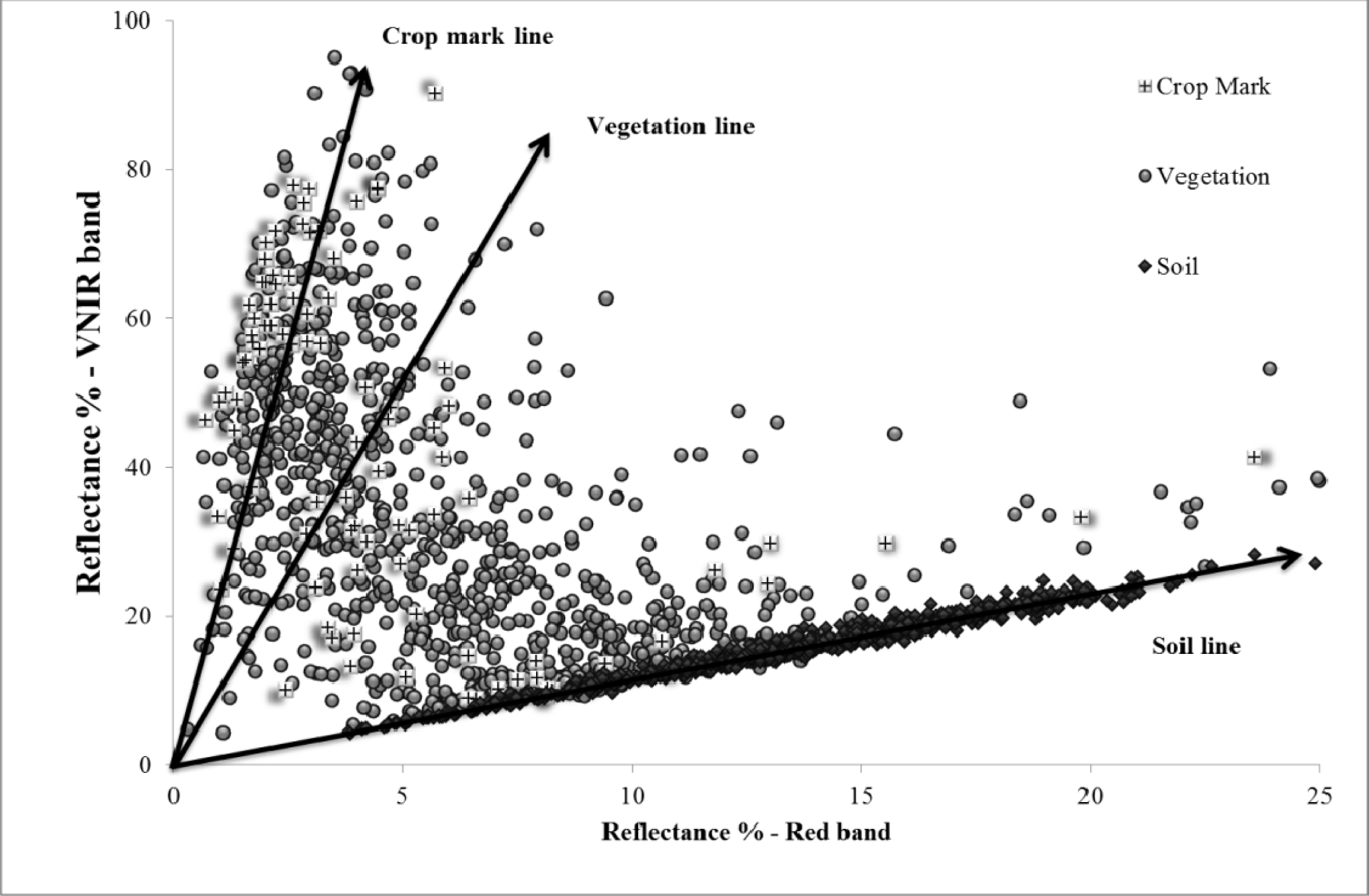
• Step 3: The next step, concerns the definition by the user of the spectral data used in the transformation. As it is shown in Figure 5, three types of dataset were determined by the user: soil, vegetation and crop marks. Major concerns can been outstretched–similar to those of the T-K transformation-since the basis vectors depend on the data set selected to construct the transform. In order to overcome such limitations a large dataset has been evaluated, taking into consideration the dynamic nature of the formation of crop marks. In addition, the basis vectors were selected based on the results from previous studies performed by the authors [21,45]. Indeed, the data selected were taken during the best phenophase (time-window) where crop marks are enhanced (boot stage of the crops).
• Step 4: After the basis vectors were defined, rotation of the PCA n-space was performed into a new 3D orthogonal space (soil; vegetation; crop marks). In the end, the coefficients for all satellite sensors were calculated based on the 3D rotation angles. These coefficients are expected to enhance crop marks, vegetation and soil for each specific sensor selected.

3. Results

For each sensor, three new linear equations were derived. The coefficients for each sensor are shown in the following Equations (3)–(23). As it is obvious from Figure 6, these coefficients tend to be very similar for each dataset, but not exactly the same. Therefore, new coefficients should be calculated for each sensor as in the case of the T-K transformation. A new RGB pseudo color image can be generated after the application of this transformation. The first band is called “crop mark component”, the second band “vegetation component” and the third band “soil component”. These equations are linear combinations of the VNIR bands of each sensor.

$$\mathit{Crop}\hspace{0.17em}{\mathit{mark}}_{\mathit{GeoEye}-1}=-0.39\hspace{0.17em}{\rho }_{\mathit{blue}}-0.73\hspace{0.17em}{\rho }_{\mathit{green}}+0.17\hspace{0.17em}{\rho }_{\mathit{red}}-0.54\hspace{0.17em}{\rho }_{\mathit{NIR}}$$

(3)

$${\mathit{Vegetation}}_{\mathit{GeoEye}-1}=-0.35\hspace{0.17em}{\rho }_{\mathit{blue}}-0.37\hspace{0.17em}{\rho }_{\mathit{green}}-0.68\hspace{0.17em}{\rho }_{\mathit{red}}+0.54\hspace{0.17em}{\rho }_{\mathit{NIR}}$$

(4)

$${\mathit{Soil}}_{\mathit{GeoEye}-1}=0.08\hspace{0.17em}{\rho }_{\mathit{blue}}+0.27\hspace{0.17em}{\rho }_{\mathit{green}}-0.71\hspace{0.17em}{\rho }_{\mathit{red}}-0.65\hspace{0.17em}{\rho }_{\mathit{NIR}}$$

(5)

$$\mathit{Crop}\hspace{0.17em}{\mathit{mark}}_{\mathit{ASTER}}=0.36\hspace{0.17em}{\rho }_{\mathit{green}}-0.64\hspace{0.17em}{\rho }_{\mathit{red}}-0.67\hspace{0.17em}{\rho }_{\mathit{NIR}}$$

(6)

$${\mathit{Vegetation}}_{\mathit{ASTER}}=-0.46\hspace{0.17em}{\rho }_{\mathit{green}}-0.75\hspace{0.17em}{\rho }_{\mathit{red}}+0.47\hspace{0.17em}{\rho }_{\mathit{NIR}}$$

(7)

$${\mathit{Soil}}_{\mathit{ASTER}}=-0.81\hspace{0.17em}{\rho }_{\mathit{green}}+0.14\hspace{0.17em}{\rho }_{\mathit{red}}-0.57\hspace{0.17em}{\rho }_{\mathit{NIR}}$$

(8)

$$\mathit{Crop}\hspace{0.17em}{\mathit{mark}}_{\mathit{IKONOS}}=-0.49\hspace{0.17em}{\rho }_{\mathit{blue}}-0.61\hspace{0.17em}{\rho }_{\mathit{green}}+0.24\hspace{0.17em}{\rho }_{\mathit{red}}-0.58\hspace{0.17em}{\rho }_{\mathit{NIR}}$$

(9)

$${\mathit{Vegetation}}_{\mathit{IKONOS}}=-0.38\hspace{0.17em}{\rho }_{\mathit{blue}}-0.44\hspace{0.17em}{\rho }_{\mathit{green}}-0.64\hspace{0.17em}{\rho }_{\mathit{red}}+0.51\hspace{0.17em}{\rho }_{\mathit{NIR}}$$

(10)

$${\mathit{Soil}}_{\mathit{IKONOS}}=0.18\hspace{0.17em}{\rho }_{\mathit{blue}}+0.17\hspace{0.17em}{\rho }_{\mathit{green}}-0.73\hspace{0.17em}{\rho }_{\mathit{red}}-0.63\hspace{0.17em}{\rho }_{\mathit{NIR}}$$

(11)

$$\mathit{Crop}\hspace{0.17em}{\mathit{mark}}_{\mathit{Landsat}\hspace{0.17em}4\hspace{0.17em}\mathit{TM}}=-0.39\hspace{0.17em}{\rho }_{\mathit{blue}}-0.60\hspace{0.17em}{\rho }_{\mathit{green}}+0.31\hspace{0.17em}{\rho }_{\mathit{red}}-0.62\hspace{0.17em}{\rho }_{\mathit{NIR}}$$

(12)

$${\mathit{Vegetation}}_{\mathit{Landsat}\hspace{0.17em}4\hspace{0.17em}\mathit{TM}}=-0.40\hspace{0.17em}{\rho }_{\mathit{blue}}-0.50\hspace{0.17em}{\rho }_{\mathit{green}}-0.66\hspace{0.17em}{\rho }_{\mathit{red}}+0.40\hspace{0.17em}{\rho }_{\mathit{NIR}}$$

(13)

$${\mathit{Soil}}_{\mathit{Landsat}\hspace{0.17em}4\hspace{0.17em}\mathit{TM}}=0.17\hspace{0.17em}{\rho }_{\mathit{blue}}+0.23\hspace{0.17em}{\rho }_{\mathit{green}}-0.68\hspace{0.17em}{\rho }_{\mathit{red}}-0.67\hspace{0.17em}{\rho }_{\mathit{NIR}}$$

(14)

$$\mathit{Crop}\hspace{0.17em}{\mathit{mark}}_{\mathit{Landsat}\hspace{0.17em}7\hspace{0.17em}\mathit{ETM}+}=-0.42\hspace{0.17em}{\rho }_{\mathit{blue}}-0.69\hspace{0.17em}{\rho }_{\mathit{green}}+0.21\hspace{0.17em}{\rho }_{\mathit{red}}-0.55\hspace{0.17em}{\rho }_{\mathit{NIR}}$$

(15)

$${\mathit{Vegetation}}_{\mathit{Landsat}\hspace{0.17em}7\hspace{0.17em}\mathit{ETM}+}=-0.34\hspace{0.17em}{\rho }_{\mathit{blue}}-0.41\hspace{0.17em}{\rho }_{\mathit{green}}-0.65\hspace{0.17em}{\rho }_{\mathit{red}}+0.53\hspace{0.17em}{\rho }_{\mathit{NIR}}$$

(16)

$${\mathit{Soil}}_{\mathit{Landsat}\hspace{0.17em}7\hspace{0.17em}\mathit{ETM}+}=0.12\hspace{0.17em}{\rho }_{\mathit{blue}}+0.22\hspace{0.17em}{\rho }_{\mathit{green}}-0.73\hspace{0.17em}{\rho }_{\mathit{red}}-0.64\hspace{0.17em}{\rho }_{\mathit{NIR}}$$

(17)

$$\mathit{Crop}\hspace{0.17em}{\mathit{mark}}_{\mathit{QuickBird}}=-0.39\hspace{0.17em}{\rho }_{\mathit{blue}}-0.71\hspace{0.17em}{\rho }_{\mathit{green}}+0.21\hspace{0.17em}{\rho }_{\mathit{red}}-0.55\hspace{0.17em}{\rho }_{\mathit{NIR}}$$

(18)

$${\mathit{Vegetation}}_{\mathit{QuickBird}}=-0.36\hspace{0.17em}{\rho }_{\mathit{blue}}-0.40\hspace{0.17em}{\rho }_{\mathit{green}}-0.65\hspace{0.17em}{\rho }_{\mathit{red}}+0.53\hspace{0.17em}{\rho }_{\mathit{NIR}}$$

(19)

$${\mathit{Soil}}_{\mathit{QuickBird}}=0.09\hspace{0.17em}{\rho }_{\mathit{blue}}+0.24\hspace{0.17em}{\rho }_{\mathit{green}}-0.72\hspace{0.17em}{\rho }_{\mathit{red}}-0.65\hspace{0.17em}{\rho }_{\mathit{NIR}}$$

(20)

$$\mathit{Crop}\hspace{0.17em}{\mathit{mark}}_{\mathit{WorldView}-2}=-0.38\hspace{0.17em}{\rho }_{\mathit{blue}}-0.71\hspace{0.17em}{\rho }_{\mathit{green}}+0.20\hspace{0.17em}{\rho }_{\mathit{red}}-0.56\hspace{0.17em}{\rho }_{\mathit{NIR}}$$

(21)

$${\mathit{Vegetation}}_{\mathit{WorldView}-2}=-0.37\hspace{0.17em}{\rho }_{\mathit{blue}}-0.39\hspace{0.17em}{\rho }_{\mathit{green}}-0.67\hspace{0.17em}{\rho }_{\mathit{red}}+0.52\hspace{0.17em}{\rho }_{\mathit{NIR}}$$

(22)

$${\mathit{Soil}}_{\mathit{WorldView}-2}=0.09\hspace{0.17em}{\rho }_{\mathit{blue}}+0.27\hspace{0.17em}{\rho }_{\mathit{green}}-0.71\hspace{0.17em}{\rho }_{\mathit{red}}-0.65\hspace{0.17em}{\rho }_{\mathit{NIR}}$$

(23)

The proposed transformation will be able to highlight the difference between the crops marks and the healthy vegetation as well as to the background soil. In addition, the initial information of the satellite data is minimized only to the VNIR part of the spectrum.

For assessment purposes of these linear transformations, data gathered from the Alampra test field were used. These values were plotted against the NDVI index (Figures 7 and 8, respectively). A strong linear regression (R² > 0.91) between 2nd component (vegetation) and the NDVI index was found (Figure 7). This linear relationship was expected since the second component aims to enhance healthy vegetation, similarly with the NDVI index. Moreover, some fluctuations of the distribution of the second component values are also noticed for the different types of dataset, as a result of the different spectral capabilities of each sensor. However, the case is not similar for the first component. As it is shown in Figure 8, the formation of crop marks, related with the NDVI value and the phenological cycle, is very complicated to be modeled, as already concluded by many researchers (see Section 1). Therefore, the proposed first component may be used as a separately tool for the detection of crop marks and has no linear correlation with existing vegetation indices.

4. Evaluation

In order to evaluate the proposed transformations for each sensor, different archaeological sites were evaluated as shown in Figure 2. These sites are located in SW Cyprus and southern-central Greece. The selection of these archaeological sites was mainly based on the knowledge of the area—which is very important for the detection of crop marks—as well as on the accessibility of the different types of satellite data. In detail, IKONOS image was used in the case of Nea Paphos at SW Cyprus, a GeoEye-1 and a QuickBird images at the Elis archeological site. Megalopolis archaeological site was examined using the WorldView-2 data. Finally, free distributed images Landsat 4 TM and Landsat 7 ETM+ from USGS Glovis and a medium resolution ASTER image were evaluated in the case of Thessaly.

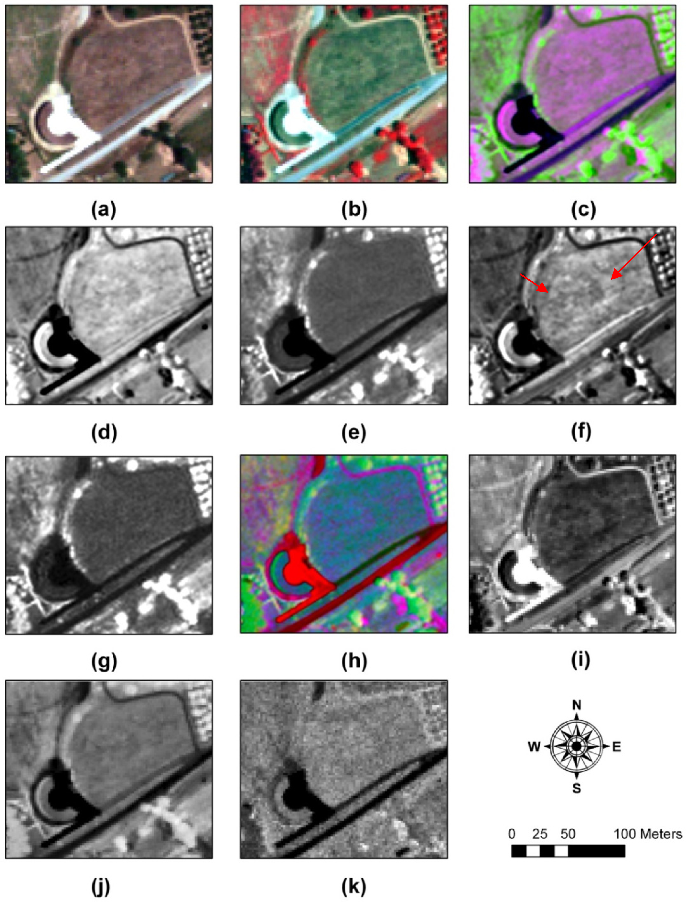
In each case, different existing algorithms, vegetation indices and false composites were compared with the proposed linear transformations of this study. Figures 9 and 16 present the results from the application of linear equations (d–f), as well the RGB pseudo composite of the proposed transformation components (c). In addition, RGB and NIR-R-G composites are presented (a and b, respectively in each figure), and the result from the NDVI index (g). Finally, the results from the PCA analysis are also displayed (h–k).

In general, the results show that high resolution satellite images tend to give better outcomes mainly due to their smaller pixel size. Indeed, as it is presented in Figures 12 and 14, the interpretation of medium resolution satellite images (Landsat 4 TM; Landsat 7 ETM+ and ASTER) can be problematic due to mixed pixels as a result of the spatial resolution of these satellite data. Interpretation of satellite data is considered to be very important task for identification of buried archaeological features. Indeed, for the detection of crop marks experts used a variety of interpretation keys such as shape, length, shadow, color as well the archaeological knowledge of the case study area.

A circular crop mark at the western part of a modern theater within the archaeological site of Elis can be seen in Figure 9 using the GeoEye-1 satellite image. Both the first and the third components of the proposed transformation (Figure 9d,f, respectively) tend to enhance the results more so compared to other algorithms. It should be noted that NDVI index tends to give very poor results (Figure 9g) and therefore this crop mark cannot be detected relying on it. In contrast, crop mark is noticeable in the first PCA component (Figure 9i). RGB and NIR R–G composites (Figure 9a,b, respectively) seem to highlight a part of the circular crop mark. The extensive archaeological site of ancient Elis comprises the ancient agora, the theatre, the residential sector, the cemeteries, the acropolis, and the unexcavated gymnasiums. A number of settlements or suburbs, each with its own cemetery, developed around the city. However, as archaeologists mention, only small sections of the city have been investigated so far [46]. This circular crop mark with radius almost 50 m seems to be a part of the Elis’s archaeological site, since further to its shape, the mark is in close proximity with the ancient theatre (150 m to the east and 500 m north east from the ancient agora).

In addition to the above, two interesting linear features can be also detected in Figure 10, from the same archaeological site using again the GeoEye-1 satellite imagery. A linear feature with direction from N–S seems to continue from an already excavated area at the northern part. At the center of this feature, another linear finding, perpendicular to the previous one has been also detected. Although both linear features are detectable to several algorithms applied to the GeoEye-1 image, the second component of the proposed transformation (Figure 10e) tends to further enhance these buried archaeological features. The QuickBird analysis, for the same area of interest, has indicated a new linear feature with direction from W–E (Figure 11) different from the previous analysis. This feature is visible to the first and third component of the proposed transformation (Figure 11d,f, respectively). In addition, another linear feature with direction NW–S has been recognized. These features are in some parts visible to the 2nd PCA component (Figure 11j). The previous results from the Elis archaeological site, highlight the dynamic formation of crop marks since some buried archaeological features may be visible in some periods only. Therefore, multi-temporal analysis for the detection of crop marks is necessary to enrich the outcome results. All these linear features seem to be correlated with the existing excavated ancient agora at the north. The linear feature with direction N–S at Figure 10 appears to be a continuation of an already existing road of the agora and with similar dimensions (≈6 m). The perpendicular features in Figures 10 and 11 seem to in parallel with the orientation of the excavated ancient agora. The overall interpretation of the satellite images for the archaeological site of Elis (Figures 9 and 11) in relation with the excavated part of the site indicate interesting indications for the existence of buried archaeological remains

As a circular feature, typical Neolithic tell in the Thessalian plain (called magoula) can be seen in Figure 12 using ASTER image. The Thessalian region located in north Greece is considered as the primary agricultural area of Greece. At this plain, many of Neolithic settlements/tells called magoules were established from the early Neolithic period until the Bronze Age (6000–3000 BC). The tells are typically low hills of 1–5 m height above the surrounding area and they mainly consist of loam and mud based materials. Several magoules are located all over Thessaly and can be found within different kinds of vegetation. Due to the intensive cultivation of the land in the past and their low elevation, a major number of them are not clearly visible from the ground [7,8]. Several studies performed in this area have demonstrated the potentials of remote sensing techniques—with varying degrees of success—for the detection of Neolithic tells [7,8,21,22,47].

This tell cannot be detected in NDVI algorithm (Figure 12g) while the first PCA components tend to over-saturate the image (Figure 12i). False composite of the proposed transformation (Figure 12c) enhances the magoula as well as all three different components of the ASTER linear transformation (Figure 12d–f). Furthermore, the proposed transformation highlights the outline of the tell against the surrounding cultivated area. The Thessalian plain was also examined for the rest of the medium resolution satellite images: Landsat 4 TM (Figure 13) and Landsat 7 ETM+ (Figure 14). As it is clearly shown, the proposed transformations for these data were able to detect the circular Neolithic tell, in contrary with the NDVI index which seems to be problematic in the case of Landsat 4 TM (Figure 13g). The PCA transformation provides the ability to detect tells in both satellite images.

An extensive elliptical shape at the UNESCO World Heritage archaeological site of Nea Paphos in Cyprus, has been marked from the high resolution IKONOS image (Figure 15). Nea Paphos is situated on a small promontory on the southwest coast of the island. According to written sources, the town was founded at the end of the fourth century by Nicocles, the last king of Palaepaphos (Old Paphos). In the beginning of the third century B.C. when Cyprus became part of the Ptolemaic kingdom, which had its capital in Alexandria, Nea Paphos became the center of Ptolemaic administration on the island. Systematic excavations at Nea Paphos started in 1962 by the Department of Antiquities of Cyprus during which many of the ancient town’s administrative buildings as well as private houses and ecclesiastical buildings came to light. The elliptical feature, due to its large dimension (60 × 30 m), can be easily recognized from the space or using aerial image. However, despite its size, NDVI index (Figure 15g) could not enhance this buried archaeological feature. Fine results are noticeable in the first PCA component (Figure 15i) and the first component of the proposed transformation (Figure 15d). In addition, the boundaries of the archaeological site can be seen in Figure 15f (third component of the proposed linear transformation). The systematic observations of this elliptical mark in a series of archive satellite and aerial data (not shown in this paper) highlight the hypothesis of a buried archaeological feature (amphitheater?) with still visible marks on the surface

Finally, some linear features at the western part of excavated areas in Megalopolis archeological site (Figure 16) have been also revealed. Megalopolis was founded in 371 BC, after the cohabitation of different Arcadic hamlets with the aid of the Theban general Epameinondas. The town declined during the Late Roman period, while during the Middle Ages, its inhabitants dispersed to nearby settlements [46]. The linear features are visible to the false composite of the proposed transformation (Figure 16c), as well as to the first and third component of the transformation (Figure 16d,f, respectively). These features are also visible in the first PCA component (Figure 16i) while the rest of the images generate very poor results. These features seems to be related with previous excavations in the agora (soil heaps).

The previous results (i.e., Figures 9 and 16) have been quantified using the normalized difference between crop marks and the background area as proposed by [21] and modified by [48]. High normalized difference refers to high contrast of the archaeological feature compared to the surrounding area. Figure 17 presents the results for all sensors and archaeological sites mentioned in this paper. Further to the three components of the proposed transformation (CC1, CC2, CC3), the NDVI and the PCA1-2 were also examine and compared. The results are quite similar to the conclusions of the interpretation results as discuss before. In general, the proposed transformation (CC1–CC3) seems to enhance the detection of crop marks more so than the rest of the algorithms. It is also interesting to note the difference observed between the proposed transformation and the NDVI index. Although PCA analysis tends to give high scores of difference, these are less with the proposed transformation. In some cases (e.g., GeoEye-1), the difference can be as much as 15% higher. The soil component developed in this study can be used in order to detect archaeological marks not fully vegetated (as in the case of the previous excavation in the Megalopolis.

5. Conclusions

Remote sensing has been widely explored during the last decade for supporting archaeological research. The detection of un-excavated archaeological sites has been long attracted the interest of scientists, while the new capabilities of satellite remote sensing sensors provide further possibilities. However, the identification of buried relics which is mainly based on interpretation of images is not an easy task. For this reason, many researchers have applied known image analysis algorithms in order to improve the interpretation. However, these algorithms have not been developed for this purpose and, therefore, their success can vary.

In contrast, this paper aims to introduce new linear equations for seven different satellite images (QuickBird; IKONOS; WorldView-2; GeoEye-1, ASTER; Landsat 4 TM and Landsat 7 ETM+) for the enhancement of crop marks. Therefore, these equations aim to enhance the detection of crop marks which are related to buried archaeological features.

These linear equations have been developed using a large dataset of simulated data. The data have been recorded using a handheld spectroradiometer (GER 1500) and several campaigns were performed during the phenological cycle of the crops. The narrowband reflect cane values taken from the spectroradiometer have been resampled in all the above mentioned sensors using the appropriate Relative Response Filter (RSR). Then, Principal Component Analysis (PCA) was carried out in order to detect the initial axes of the three components of the proposed transformation: crop mark, vegetation and soil. These vectors were rotated in order to enhance the final outcomes. All linear transformations were evaluated in different existing archaeological sites in Cyprus and Greece. As it was found in all cases, the proposed equations were able to enhance the detection of crop marks. Indeed, the results have highlighted the benefits of the proposed transformations, in contrast to other existing algorithms. In addition, as it was found, these equations were able to detect crop marks, where at the same time, NDVI index generated poor results.

The linear equations provided in this paper can be applied in different archaeological sites using different satellite data nowadays available for scientists. In addition, Landsat 4 TM and Landsat 7 ETM+ equations are also provided since such kind of sensors can provide historical images of an archaeological site. Although several crop marks can be also detected using aerial images with better spatial resolution, the use of satellite images can be also used for providing additional information to archaeologists. Indeed, in areas where aerial data are not regularly acquired or not specifically acquired for archaeological investigations, satellite images seem ideal to support archaeological research. This is the case of Mediterranean countries where the need for such information is essential due to the vast anthropogenic changes in the archeolandscapes.

The main disadvantage of the methodology is the fact that for each different type of sensors a new equation needs to be developed. In this paper, some of the most promising and well known satellite data have been studied in order to provide the appropriate equations to the scientific community. Indeed, some interesting crop marks have been revealed using the proposed transformations in different archaeological sites. New satellite sensors can be considered using these ground simulated data, while at the same time an evaluation of satellite sensors ready for launch (e.g., Sentinel) can be also studied.