Sparse Frequency Diverse MIMO Radar Imaging for Off-Grid Target Based on Adaptive Iterative MAP

Abstract

The frequency diverse multiple-input-multiple-output (FD-MIMO) radar synthesizes a wideband waveform by transmitting and receiving multiple frequency signals simultaneously. For FD-MIMO radar imaging, conventional imaging methods based on Matched Filter (MF) cannot enjoy good imaging performance owing to the few and incomplete wavenumber-domain coverage. Higher resolution and better imaging performance can be obtained by exploiting the sparsity of the target. However, good sparse recovery performance is based on the assumption that the scatterers of the target are positioned at the pre-discretized grid locations; otherwise, the performance would significantly degrade. Here, we propose a novel approach of sparse adaptive calibration recovery via iterative maximum a posteriori (SACR-iMAP) for the general off-grid FD-MIMO radar imaging. SACR-iMAP contains three loop stages: sparse recovery, off-grid errors calibration and parameter update. The convergence and the initialization of the method are also discussed. Numerical simulations are carried out to verify the effectiveness of the proposed method.

1. Introduction

The multiple-input-multiple-output (MIMO) radar system has attracted much attention recently, due to the additional degrees of freedom and the higher spatial resolution [1]. Through space diversity, the whole array aperture is extended by virtual sensors, which are equivalently constructed by different combinations of transmitters and receivers. The MIMO radar system with frequency diversity (FD-MIMO) has been researched widely in the recent years [2–4], since its range resolution can be further improved by simultaneously fusing the echoes coming from different transmitters to form a wideband signal [5]. Hence, here we focus our research on the FD-MIMO radar imaging.

For a restricted number of transmitters and receivers, the wavenumber-domain coverage is incomplete, so the traditional imaging methods based on matched filter (MF) fail to achieve good performance. Nonetheless, in most radar imaging applications, the scatterers of the target are often distributed sparsely, i.e., the number of actual scatterers is much smaller than that of the potential scatterers. Much existing research has been dedicated to sparse recovery techniques for MIMO radar imaging [6–8], such as orthogonal matching pursuit (OMP) and basis pursuit (BP). Based on compressive sensing (CS), higher resolution and better imaging performance can be obtained by exploiting the sparsity of the scatterers.

However, most existing sparse recovery techniques require the scatterers to be located exactly on the pre-discretized grid. When off-grid scatterers exist, their performance would be severely affected. In MIMO radar imaging [6,9], since the scatterers are distributed in a continuous scene, the off-grid problem usually emerges, even if the discretized grid is dense, which would lead to the mismatch of the sensing matrix. Using a denser grid may alleviate the mismatch level; however, it is still not an advisable remedy for the off-grid target imaging, since a denser grid may dramatically enhance the coherence between the column of the sensing matrix, which causes the violation of the restricted isometry property (RIP) condition for reliable sparse recovery. Therefore, in this paper, we consider more practical situations with off-grid scatterers for the FD-MIMO radar imaging.

For linear measurement equation y = ϕx + e, the perturbed CS problem, where the sensing matrix ϕ is unknown or subject to an unknown perturbation, has been a hot research topic. Gleichman and Eldar [10] introduce a concept named blind CS, where the sensing matrix is assumed unknown. Chi et al.[11] analyze the performance of CS methods when the mismatch of the sensing matrix exists and verify that the sparse recovery performance is likely to suffer from a large error when the mismatch is large. However, the research in [10,11] is limited to theoretical analysis of the performance loss and does not devise any modified approaches. Hereafter, some algorithms have been proposed to deal with the mismatch of the sensing matrix and have some practical application to off-grid direction of arrival (DOA) estimation. Zhu et al.[12] propose a feasible approach, named sparse total least squares (S-TLS), to alleviate the effect of mismatch, which, however, is inefficient and time-consuming. Han et al.[13] introduce faster and more robust algorithms, total least-squares Focal Underdetermined System Solver (TLS-FOCUSS) and Synchronous Descending Focal Underdetermined System Solver (SD-FOCUSS), then apply SD-FOCUSS to the DOA multiple measurement vectors (MMV) model. From the Bayesian perspective, S-TLS in [12] and TLS-FOCUSS, SD-FOCUSS in [13] are all equivalent to obtaining a maximum a posteriori (MAP) solution by assuming that the mismatch errors are white Gaussian distributed. However, since we do not have enough priori information about the scatterer distribution of the target, a uniform distribution of the off-grid error conforms more to a practical physical situation than a Gaussian distribution when we make arbitrary discretization of the imaging area. Yang et al.[14] formulate the off-grid DOA estimation problem using sparse Bayesian inference (SBI) and recover the source signal and the matrix mismatch through expectation-maximization (EM) iteration. In SBI, the unknown solutions are assumed to be time-varying; however, during the short imaging time, the reflection coefficients of the scatterers to be solved are time-invariant. Hence, a new algorithm needs to be developed to take into account the time-invariant unknowns.

In this paper, we propose an approach of sparse adaptive calibration recovery via iterative maximum a posteriori (SACR-iMAP) for the off-grid FD-MIMO radar imaging. As a matter of fact, SACR-iMAP is within the framework of Bayesian CS [15]. The off-grid error (the distance from the actual scatterer to the nearest assumed grid point) that lies within a bounded interval is assumed to be uniformly distributed rather than Gaussian distributed, as in [12,13]. SACR-iMAP adaptively calibrates the off-grid errors and, meanwhile, seeks the optimal target reconstruction results. Through iterative MAP, it turns the non-convex optimization problem of the off-grid sparse recovery to three main stages: sparse recovery, off-grid errors calibration and parameter update. The off-grid errors and the power of noise are dynamically and adaptively calibrated, which enhance the robustness of the proposed algorithm. In [16–18], the authors also linearize the off-grid errors using the first order Taylor approximation and establish an alternating process to obtain the optimized recovery results and off-grid errors estimation. However, since they have not deduced the imaging problem from the Bayesian maximum a posteriori aspect, the estimation of the power of noise is unavailable. Moreover, the proposed algorithm can reconstruct scatterers accurately even under a coarsely discretized grid.

The outline of this paper is as follows. In Section 2, the sparse recovery of the off-grid target for the FD-MIMO imaging problem is formulated. In Section 3, a novel algorithm, named SACR-iMAP, for the off-grid sparse recovery problem is proposed. In Section 4, extensive numerical simulations are presented to verify the proposed algorithm. Finally, in Section 5, the conclusions are drawn.

Notations used in this paper are as follows. Bold-case letters are reserved for vectors and matrices. ‖x‖_p denote the l_p norm of a vector x. ‖A‖₂ is the spectral norm of the matrix A. diag(x) is a diagonal matrix with its diagonal entries being the entries of a vector x. ⊙ is the Hadamard (elementwise) product. (·)^T, (·)^T and vec (·) denote the transpose, the conjugate transpose operation and the vectorization operation, respectively.

2. Problem Formulation

2.1. FD-MIMO Imaging Problem

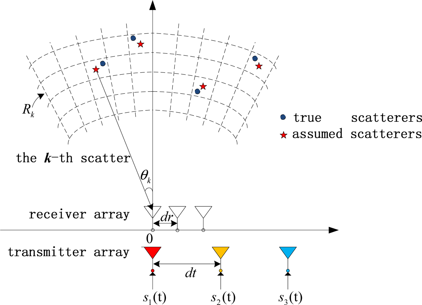
Consider the scenario of a MIMO radar system composed by M transmitters and N receivers, as illustrated in Figure 1. Here, we adopt a narrowband FD-MIMO radar system, which is proposed in [4]. Considering that the linear frequency modulated (LFM) signal has long been used in radar systems, because of its implementation simplicity, constant modulus and high range resolution [5], here, we focus our derivation on the LFM-based FD-MIMO radar imaging. The different transmitter elements transmit LFM signals within different bands, respectively.

Assuming that all of the M waveforms have an equal chirp rate, and letting s_m(t) (for m = 1,2,...,M) be the transmitted LFM waveform for the m-th transmitter, therefore, we have:

$$s_m\left(t\right)=\mathit{rect}\left(\frac{t}{T}\right)\text{exp}\left[\text{j}2\pi \left(f_{m}t+\frac{1}{2}\gamma t^2\right)\right]$$

(1)

where γ is the chirp rate and f_m is the carrier frequency of the m-th transmitter. For reducing the complexity of the hardware system, we consider f_m satisfies [5]:

$$f_m=f_c+m\gamma T$$

(2)

where f_c and T represent the reference carrier frequency and the pulse temporal width, respectively, and:

$$\mathit{rect}\left(\frac{t}{T}\right)=\{\begin{array}{ll}1\hfill & \left|t\right|\le T/2\hfill \\ 0\hfill & \left|t\right|>T/2\hfill \end{array}$$

(3)

Suppose the imaging scene contains U radial range bins and V angle bins. Setting K = UV, we define σ_k, R_k, θ_k (for k= 1,2,...,K) as the complex reflection coefficient, the radial range and the impinging angle (relative to the array normal), respectively. By defining s(t) = [s₁(t), s₂(t), …, s_M(t)]^T, the echoes of N receivers z(t) = [z₁(t), z₂(t), …, z_N(t)]^T can be written in the following form:

$$\mathit{z}\left(t\right)=\sum _{k=1}^K{\sigma }_k\mathit{b}\left({\theta }_k\right){\mathit{a}}^T\left({\theta }_k\right)\mathit{s}\left(t-\frac{2R_k}{c}\right)+\mathit{e}\left(t\right)$$

(4)

where e(t) is the additive noise. The terms {a(θ_k)} and {b(θ_k)} refer to the transmit and receive steering vectors, respectively. Assuming that the bandwidth of each LFM signal B = γT is narrow and that the imaging scene is small, then {a(θ_k)} and {b(θ_k)} can be described by Equations (5) and (6):

$$\mathit{a}\left({\theta }_k\right)={\left[1,\text{exp}\left(j\frac{2\pi d_{t2}{\theta }_k}{\lambda }\right),\cdots ,\text{exp}\left(j\frac{2\pi d_{tM}{\theta }_k}{\lambda }\right)\right]}^T$$

(5)

$$\mathit{b}\left({\theta }_k\right)={\left[1,\text{exp}\left(j\frac{2\pi d_{r2}{\theta }_k}{\lambda }\right),\cdots ,\text{exp}\left(j\frac{2\pi d_{rN}{\theta }_k}{\lambda }\right)\right]}^T$$

(6)

where λ represents the reference carrier wavelength and λ = c/f_c and d_ti (i = 2, …, M) represent the distance from the i-th transmitter to the first transmitter and d_ri (i = 2, …, N) represent the distance from the i-th receiver to the first receiver.

After orthogonal separation, we can obtain the received signal of the mn-th virtual sensor corresponding to the m-th transmitter and the n-th receiver as:

$$z_{mn}\left(t\right)=\sum _{k=1}^K{\sigma }_k{b}_n\left({\theta }_k\right)a_m\left({\theta }_k\right)s_m\left(t-\frac{2R_k}{c}\right)+e_{mn}\left(t\right)$$

(7)

where a_m(θ_k) is the m-th element of {a(θ_k)}, b_n(θ_k) is the n-th element of {b(θ_k)} and e_mn(t) is the corresponding noise after orthogonal separation.

Supposing that the reference range is R₀, for LFM signal, we have:

$$s_m\left(t-\frac{2R_k}{c}\right)s_m^{*}\left(t-\frac{2R_0}{c}\right)\approx \text{rect}\left(\frac{t-2R_0/c}{T}\right)\text{exp}\left\{-j\frac{4\pi }{c}\left[\left(f_m+\gamma t^{\prime }\right)r_k-\frac{\gamma }{c}{r}_k^2\right]\right\}$$

(8)

where t′ = t − 2R₀/c and r_k = R_k − R₀. After dechirping and removing the residual video phase in Equation (8) according to [19], for the q-th (q = 1,2,...,Q) snapshot, combing Equations (5) and (6) with Equations (7) and (8), we have:

$$z_{mn}\left(q\right)=\sum _{k=1}^K{\sigma }_k\text{exp}\left\{-j2\pi \left[\frac{2\left(f_m+\gamma t_q^{\prime }\right)}{c}{r}_k-\frac{d_{tm}+d_{rn}}{\lambda }{\theta }_k\right]\right\}+e_{mn}\left(q\right)$$

(9)

Here, we consider uniform linear arrays (ULA) for the transmitters and receivers with d_t = Nd and d_r = d, where d_t and d_r refer to the distances between adjacent transmitting and receiving antennas, respectively. So, we can get d_tm + d_rn = ((m − 1)N + n − 1)d. What is more, the corresponding derivation of ULA in this paper can be directly generalized to other configurations of the transceiver array.

Define z = vec(z_mn(q)) with its size MNQ × 1, e = vec(e_mn(q)) with the same size, then set:

$${\mathit{h}}_k=\mathit{vec}\left(\text{exp}\left(-j2\pi \left(\frac{2\left(f_m+\gamma t_q^{\prime }\right)}{c}{r}_k-\frac{d_{tm}+d_{rn}}{\lambda }{\theta }_k\right)\right)\right)$$

(10)

Moreover, we let:

$$\mathit{H}=\left(\begin{array}{cccc}{\mathit{h}}_1& {\mathit{h}}_2& \cdots & {\mathit{h}}_K\end{array}\right)$$

(11)

Defining σ = [σ₁,…,σ_K], then the echoes can be redefined as:

$$\mathit{z}=\mathit{H}\mathit{\sigma }+\mathit{e}$$

(12)

The available observations in the wavenumber domain point are (2(f_m + γt′_q)/c, ((m − 1)N + n − 1)d/λ) (m = 1,…,M, n = 1,…,N, q = 1,…,Q) [20], which are too few to achieve good recovery performance by traditional imaging methods based on matched filter (MF). However, for most targets, especially those in the air, the number of actual scatterers is much smaller than that of potential scatterers. Therefore, the sparsity of the target is an appropriate priority by which more accurate imaging performance can be expected. Herein, we consider utilizing the sparsity of the scatterers to realize high resolution imaging.

2.2. Sparse Recovery of the Off-Grid Target for FD-MIMO Imaging Problem

In most cases of radar imaging, the scatterers are distributed in a continuous scene. The sparsity is more of a kind of quantitative description. However, if we use the sparsity prior directly into Equation (12), the off-grid problem would emerge, which means that, no matter how densely we discretize the imaging scene, the scatterers could be off-grid. To alleviate the effect of the off-grid problem on the performance of the sparse recovery, we must make some amendments to Equation (12). Considering the off-grid problem, we have:

$$r_{k0}=r_k+\Delta r_k,{\theta }_{k0}={\theta }_k+\Delta {\theta }_k$$

(13)

where (r_k0, θ_k0) is the actual location of the k-th scatterers, (r_k, θ_k) is the assumed location and {Δr_k, Δθ_k} is the off-grid error.

Substituting Equations (2) and (13) into Equation (9), the echoes can be redefined as:

$$z_{mn}\left(q\right)=\sum _{k=1}^K{\sigma }_k\text{exp}\left\{-j2\pi \left[\frac{2\left(f_c+m\gamma T+\gamma t_q^{\prime }\right)}{c}\left(r_k+\Delta r_k\right)-\frac{d_{tm}+d_{rn}}{\lambda }\left({\theta }_k+\Delta {\theta }_k\right)\right]\right\}+e_{mn}\left(q\right)$$

(14)

Since the off-grid errors are restricted in the region of one radial range bin or angle bin, we can assume that the off-grid errors are significantly small; then, we can make the following approximations by the Taylor expansion:

$$\begin{array}{l}\text{exp}\left(-j2\pi \cdot \frac{2\left(m\gamma T+\gamma t_q^{\prime }\right)}{c}\Delta r_k\right)\approx 1-j2\pi \cdot \frac{2\left(m\gamma T+\gamma t_q^{\prime }\right)}{c}\Delta r_k\\ \text{exp}\left(j2\pi \cdot \frac{d_{tm}+d_{rn}}{\lambda }\Delta {\theta }_k\right)\approx 1+j2\pi \cdot \frac{d_{tm}+d_{rn}}{\lambda }\Delta {\theta }_k\end{array}$$

(15)

Since {Δr_k, Δθ_k} are small, we ignore the cross-term about Δr_k, Δθ_k. Thus, we can approximate the sensing matrix as a linear combination of the errors {Δr_k, Δθ_k}:

$${\widehat{h}}_k\approx h_k\odot \mathit{vec}(1-j2\pi \times \frac{2\left(m\gamma T+\gamma t_q^{\prime }\right)}{c}\Delta r_k+j2\pi \times \frac{d_{tm}+d_{rn}}{\lambda }\Delta {\theta }_k$$

(16)

Define ĥ_1k ≈ h_k ⊙ vec(−j4π(mγT + γt′_q)/c), ĥ_2k ≈ h_k ⊙ vec(j2π(d_tm + d_rn)/λ), Λr = diag(Δr_k), Λθ = diag(Δθ_k), for k = 1, 2, ..., K. Moreover, we let:

$$\begin{array}{c}\widehat{H}=\left({\widehat{h}}_{11}{\widehat{h}}_{12}\cdots {\widehat{h}}_{1K}{\widehat{h}}_{21}{\widehat{h}}_{22}\cdots {\widehat{h}}_{2K}\right)\\ \Lambda ={\left(\Lambda r\hspace{0.17em}\hspace{0.17em}\Lambda \theta \right)}^T\\ {\sigma }^{\prime }=\sigma \odot \text{exp}\left(-j\frac{4\pi f_c}{c}\Delta r_k\right)\end{array}$$

(17)

Then, we can get the matrix-vector form corresponding to Equation (14):

$$\mathit{z}=\left(\mathit{H}+\widehat{\mathit{H}}\mathit{\Lambda }\right){\mathit{\sigma }}^{\prime }+\mathit{e}$$

(18)

Thus, our pursuit is to find out the optimized σ′ and Λ; then, we can get the corresponding reflection coefficients σ. We cast both σ′ and Λ as unknown parameters and search for the sparsest solution and simultaneously estimate the off-grid errors.

3. SACR-iMAP Algorithm

3.1. Basic Idea of the Proposed Algorithm

Inheriting the Bayesian idea, we can estimate σ′ and Λ via the MAP method. Suppose that the vector form of reflection coefficient of the scatterers σ is sparse, then the prior distribution of σ′ satisfies [21]:

$$\text{Pr}\left({\mathit{\sigma }}^{\prime }\right)\propto \text{exp}\left\{-{\Vert {\mathit{\sigma }}^{\prime }\Vert }_p^p\right\},\left(\mathit{for}\hspace{0.17em}\hspace{0.17em}\hspace{0.17em}\hspace{0.17em}\hspace{0.17em}\hspace{0.17em}\hspace{0.17em}0<p\le 1\right).$$

(19)

Further, suppose that e satisfies the complex normal distribution with mean zero and covariance matrix ξI (ξ is the power of the noise and I denotes the identity matrix). Assume Λr and Λθ as independent, identically uniformly distributions as follows:

$$\mathit{\Lambda }\mathit{r}~U\left({\left[-\frac{1}{2}{\rho }_r,\frac{1}{2}{\rho }_r\right]}^K\right),\mathit{\Lambda }\mathit{\theta }~U\left({\left[-\frac{1}{2}{\rho }_{\theta },\frac{1}{2}{\rho }_{\theta }\right]}^K\right)$$

(20)

where ρ_r and ρ_θ are the radial range bin interval and angle bin interval, respectively. Here, we consider estimating all of the unknowns σ′, Λ and ξ via the MAP method, which maximizes:

$$\begin{array}{l}\text{Pr}\left({\mathit{\sigma }}^{\prime },\mathit{\Lambda }\mathit{r},\mathit{\Lambda }\mathit{\theta },\xi |\mathit{z}\right)\\ \propto \text{Pr}\left(\mathit{z}|{\mathit{\sigma }}^{\prime },\mathit{\Lambda }\mathit{r},\mathit{\Lambda }\mathit{\theta },\xi \right)\cdot \text{Pr}\left({\mathit{\sigma }}^{\prime }\right)\cdot \text{Pr}\left(\mathit{\Lambda }\mathit{r}\right)\cdot \text{Pr}\left(\mathit{\Lambda }\mathit{\theta }\right)\\ \propto \frac{1}{{\left(\pi \xi \right)}^{MNQ}}\text{exp}\left\{-\frac{{\Vert \mathit{z}-\left(\mathit{H}+\widehat{\mathit{H}}\mathit{\Lambda }\right){\mathit{\sigma }}^{\prime }\Vert }_2^2}{\xi }\right\}\cdot \text{exp}\left\{-{\Vert {\mathit{\sigma }}^{\prime }\Vert }_p^p\right\}\end{array}$$

(21)

Taking the negative logarithm of Equation (21), we turn the MAP problem into the following optimization problem:

$$\begin{array}{ll}\left\{{\widehat{\mathit{\sigma }}}^{\prime },\widehat{\mathit{\Lambda }}\mathit{r},\widehat{\mathit{\Lambda }}\mathit{\theta },\widehat{\xi }\right\}\hfill & =\underset{{\mathit{\sigma }}^{\prime },\mathit{\Lambda }\mathit{r},\mathit{\Lambda }\mathit{\theta },\xi }{\text{argmin}}F\hfill \\ \hfill & =\underset{{\mathit{\sigma }}^{\prime },\mathit{\Lambda }\mathit{r},\mathit{\Lambda }\mathit{\theta },\xi }{\text{argmin}}\left\{{\Vert {\mathit{\sigma }}^{\prime }\Vert }_p^p+\frac{1}{\xi }{\Vert \mathit{z}-\left(\mathit{H}+\widehat{\mathit{H}}\mathit{\Lambda }\right){\mathit{\sigma }}^{\prime }\Vert }_2^2+MNQ\text{ln}\xi \right\}\hfill \end{array}$$

(22)

The minimization of F with respect to σ′, Λ and ξ is a complex non-linear optimization problem; therefore, we adopt an alternatively iterative method. Based on the iterative MAP idea, we propose a novel sparse recovery algorithm for more generalized off-grid FD-MIMO radar imaging, named sparse adaptive calibration recovery via iterative maximum a posteriori (SACR-iMAP).

3.2. Algorithm Description

SACR-iMAP includes mainly three steps. Defining l as the counter of iteration and assuming the l-th estimations are obtained, we alternatively optimize σ′^(l+1), the off-grid errors Λ^(l+1) and the parameter ξ^(l+1) in the (l+1)-th iteration. The detailed algorithm is stated as follows:

(1) Sparse Recovery

Assuming that Λ^(l) and ξ^(l) are obtained, we seek for the optimal σ′^(l+1) to minimize the following equivalent cost function:

$$F_1\left({{\mathit{\sigma }}^{\prime }}^{\left(l+1\right)}\right)={\xi }^{\left(l\right)}{\Vert {{\mathit{\sigma }}^{\prime }}^{\left(l+1\right)}\Vert }_p^p+{\Vert \mathit{z}-\left(\mathit{H}+\widehat{\mathit{H}}{\mathit{\Lambda }}^{\left(l\right)}\right){{\mathit{\sigma }}^{\prime }}^{\left(l+1\right)}\Vert }_2^2$$

(23)

Letting ∂F₁/∂σ′^(l+1) = 0, we have:

$${\left(\left(\mathit{H}+\widehat{\mathit{H}}{\mathit{\Lambda }}^{\left(l\right)}\right)\right)}^H\mathit{z}-{\left(\left(\mathit{H}+\widehat{\mathit{H}}{\mathit{\Lambda }}^{\left(l\right)}\right)\right)}^H\left(\mathit{H}+\widehat{\mathit{H}}{\mathit{\Lambda }}^{\left(l\right)}\right){{\mathit{\sigma }}^{\prime }}^{\left(l+1\right)}-\frac{p{\xi }^{\left(l\right)}}{2}\mathrm{\Pi }\left({{\mathit{\sigma }}^{\prime }}^{\left(l+1\right)}\right){{\mathit{\sigma }}^{\prime }}^{\left(l+1\right)}=0$$

(24)

where $\mathrm{\Pi }\left({{\mathit{\sigma }}^{\prime }}^{(l+1)}\right)={\mathit{W}}^{-2}\left({{\mathit{\sigma }}^{\prime }}^{(l+1)}\right),\mathit{W}\left({{\mathit{\sigma }}^{\prime }}^{(l+1)}\right)=\text{diag}\left\{{\left|{{\sigma }^{\prime }}_1^{(l+1)}\right|}^{1-\text{p}/2},\dots ,{\left|{{\sigma }^{\prime }}_{\text{K}}^{(l+1)}\right|}^{1-\text{p}/2}\right\}$.

From Equation (24), defining A = H + ĤΛ^(l) and α = pξ^(l)/2, we can get that:

$${{\mathit{\sigma }}^{\prime }}^{\left(l+1\right)}=\mathit{W}\left({{\mathit{\sigma }}^{\prime }}^{\left(l+1\right)}\right){\left({\left(\mathit{AW}\left({{\mathit{\sigma }}^{\prime }}^{\left(l+1\right)}\right)\right)}^H\mathit{AW}\left({{\mathit{\sigma }}^{\prime }}^{\left(l+1\right)}\right)+\alpha \mathit{I}\right)}^{-1}{\left(\mathit{AW}\left({{\mathit{\sigma }}^{\prime }}^{\left(l+1\right)}\right)\right)}^H\mathit{z}$$

(25)

Using the iterative relaxation method, we can get the recursion formula corresponding to σ′^(l+1)[22]:

$${{\mathit{\sigma }}^{\prime }}^{\left(l+1,s\right)}={\mathit{W}}^{\left(l,s\right)}{\left({\left(\mathit{A}{\mathit{W}}^{\left(l,s\right)}\right)}^H\mathit{A}{\mathit{W}}^{\left(l,s\right)}+\alpha \mathit{I}\right)}^{-1}{\left(\mathit{A}{\mathit{W}}^{\left(l,s\right)}\right)}^H\mathit{z}$$

(26)

where s is the internal iteration index, and W^(l,s=0) = W(σ′^(l)).

Moreover, considering MNQ < K, with the aid of the matrix inversion formula [23], we can obtain:

$${{\mathit{\sigma }}^{\prime }}^{\left(l+1,s\right)}={\left({\mathit{W}}^{\left(l,s\right)}\right)}^2{\mathit{A}}^H{\left(\mathit{A}{\left({\mathit{W}}^{\left(l,s\right)}\right)}^2{\mathit{A}}^H+\alpha \mathit{I}\right)}^{-1}\mathit{z}$$

(27)

to reduce the computation complexity for the inversion in Equation (26). The internal iteration about s stops when σ′^(l+1,s) converges, yielding σ′^(l+1).

(2) Off-Grid Errors Calibration

In this stage, we use σ′^(l+1) and ξ^(l) to estimate {Δr_k^(l+1), Δθ_k^(l+1)}, for k = 1,2,...,K, which are corresponding to minimizing the following equivalent cost function:

$$F_2\left({\mathit{\Lambda }}^{\left(l+1\right)}\right)={\Vert \mathit{z}-\left(\mathit{H}+\widehat{\mathit{H}}{\mathit{\Lambda }}^{\left(l+1\right)}\right){{\mathit{\sigma }}^{\prime }}^{\left(l+1\right)}\Vert }_2^2$$

(28)

Observe that if σ′_k^(l+1) = 0, then Δr_k = 0 and Δθ_k = 0, which suggests that we only need to calculate those {Δr_k^(l+1), Δθ_k^(l+1)} that correspond to σ′_k^(l+1) ≠ 0, while setting other errors to zero. Let Δ = [Δr₁,...,K, Δθ₁,...,K]^T, and:

$$\mathit{\Psi }=\widehat{\mathit{H}}\cdot \left[\begin{array}{cc}\mathit{diag}\left({{\mathit{\sigma }}^{\prime }}^{\left(l+1\right)}\right)& 0\\ 0& \mathit{diag}\left({{\mathit{\sigma }}^{\prime }}^{\left(l+1\right)}\right)\end{array}\right]$$

(29)

then, Equation (28) is equivalent to:

$${\mathit{\Delta }}^{\left(l+1\right)}=\{\begin{array}{l}\text{arg}\hspace{0.17em}\hspace{0.17em}\hspace{0.17em}\hspace{0.17em}\hspace{0.17em}\hspace{0.17em}\underset{\begin{array}{l}\mathit{\Delta }r\in {\left[-{\rho }_r,{\rho }_r\right]}^K\\ \mathit{\Delta }r\in {\left[-{\rho }_{\theta },{\rho }_{\theta }\right]}^K\end{array}}{\text{min}}{\Vert \left(\mathit{z}-{\mathit{H}}_{\mathrm{\Omega }}{\mathit{\sigma }}_{\mathrm{\Omega }}^{\prime \left(l+1\right)}\right)-{\mathit{\Psi }}_{\mathrm{\Omega }}{\mathit{\Delta }}_{\mathrm{\Omega }}^{\left(l+1\right)}\Vert }_2^2,\hspace{0.17em}\hspace{0.17em}\hspace{0.17em}\hspace{0.17em}\hspace{0.17em}\hspace{0.17em}\hspace{0.17em}\hspace{0.17em}\mathit{if}\hspace{0.17em}\hspace{0.17em}\hspace{0.17em}\hspace{0.17em}\hspace{0.17em}\hspace{0.17em}\hspace{0.17em}\hspace{0.17em}{\sigma }_k^{\prime \left(l+1\right)}\ne 0\hfill \\ 0,\hspace{0.17em}\hspace{0.17em}\hspace{0.17em}\hspace{0.17em}\hspace{0.17em}\hspace{0.17em}\hspace{0.17em}\mathit{if}\hspace{0.17em}\hspace{0.17em}\hspace{0.17em}\hspace{0.17em}\hspace{0.17em}{\sigma }_k^{\prime \left(l+1\right)}=0\hfill \end{array}$$

(30)

where Ω denotes the subscript set {k̃} corresponding to nonzero σ′_k̃^(l+1). H_Ω and ψ_Ω correspond to the k̃-th column of H and ψ, respectively; σ′_Ω^(l+1) and Δ_Ω^(l+1) correspond to the k̃-th element of σ′^(l+1) and Δ^(l+1), respectively, where k̃ ∈ Ω. From Equation (30), Λ^(l+1) can be obtained.

Equation (30) is a convex, constrained least square optimization problem, hence its optimal solution can be efficiently obtained.

(3) Parameter Update

To alleviate the effect of parameter estimation on the performance of SACR-iMAP, here, we embed a dynamically and adaptively parameter update process in SACR-iMAP. Similarly, setting ∂F/∂ξ^(l+1) = 0 leads to:

$${\xi }^{\left(l+1\right)}={\Vert \mathit{z}-\left(\mathit{H}+\widehat{\mathit{H}}{\mathit{\Lambda }}^{\left(l+1\right)}\right){{\mathit{\sigma }}^{\prime }}^{\left(l+1\right)}\Vert }_2^2/\left(MNQ\right).$$

(31)

Then, set l → l + 1 and repeat the three stages above until SACR-iMAP shows no obvious improvement.

Remark (1) The Initialization of SACR-iMAP

Here, we initialize Λ⁽⁰⁾ = 0, then, we get σ′⁽⁰⁾ by matched filter (MF). The j-th item of σ′⁽⁰⁾ satisfies:

$${\sigma }_j^{\prime \left(0\right)}={\mathit{h}}_j^H\mathit{z}/\left({\mathit{h}}_j^H{\mathit{h}}_j\right)$$

(32)

where h_j denotes the j-th column of the matrix H.

Then, we have the initial estimation of the noise power as:

$${\xi }^{\left(0\right)}={\Vert \mathit{z}-\mathit{H}{{\mathit{\sigma }}^{\prime }}^{\left(0\right)}\Vert }_2^2/\left(MNQ\right).$$

(33)

Remark(2) The Convergence of SACR-iMAP

We can conclude that the cost function F of SACR-iMAP decreases with the iteration index l. The detailed proof of this conclusion is given in the Appendix—Proof of Remark (2).

Remark(3) The Applicability and Limitation of SACR-iMAP

Though the algorithm of SACR-iMAP is deduced in the case of the FD-MIMO radar imaging scene, it is also applicable for the other imaging scenarios that can be described by Equation (18). In addition, we should also notice that Equation (18) is only approximately satisfied when the higher order terms of Taylor expansion are ignorable. When the off-grid errors turn bigger, the approximation of Equation (18) is violated, then the performance of SACR-iMAP would largely deteriorate.

Based on the above idea, SACR-iMAP can be described, as shown in

Table 1. The main steps of sparse adaptive calibration recovery via iterative maximum a posteriori (SACR-iMAP).

Sparse Adaptive Calibration Recovery via Iterative MAP (SACR-iMAP)
Input: z, H
Initialization:   Set ${{\mathit{\sigma }}^{\prime }}_j^{(0)}={\mathit{h}}_j^H\mathit{z}/\left({\mathit{h}}_j^H{\mathit{h}}_j\right),{\mathit{\Lambda }}^{(0)}=0,{\xi }^{(0)}={\Vert \mathit{z}-\mathit{H}{{\mathit{\sigma }}^{\prime }}^{(0)}\Vert }_2^2/\left(\mathit{MNQ}\right)$
Iteration (denote l as the counter of iteration): estimate σ′(l+1) by Equation (27); calculate Λ(l+1) by Equation (30); update ξ(l+1) by Equation (31); l → l +1; end: The loops are terminated when the norm of reflection coefficients changes moderately between the adjacent loop.
Output: σ′ = σ′(l+1), Λ = Λ(l+1).

.

4. Numerical Simulations

In this section, we present several numerical simulation results to illustrate the performance of the proposed algorithm. The SACR-iMAP is implemented in Matlab, and Equation (30) is solved using CVX [24]. SACR-iMAP is terminated as $\frac{{\Vert {{\sigma }^{\prime }}^{(l+1)}-{{\sigma }^{\prime }}^{(l)}\Vert }_2}{{\Vert {{\sigma }^{\prime }}^{(l)}\Vert }_2}\le 1\times {10}^{-6}$ or the maximum number of iterations, set to 50, is reached.

4.1. Verification of SACR-iMAP

The simulation conditions are given in

Table 2. Simulation conditions.

Parameter	Value
Number of transmitters M	10
Number of receivers N	10
Bandwidth of each transmitted signal B	15 MHz
Waveform pulse duration T	2 μs
Number of snapshots Q	10
Carrier frequency of the first transmitter fc	10 GHz
Inter-element spacing of the transmitters dt	0.3 m
Inter-element spacing of the receivers dr	0.03 m

. From Table 2, we know that the wavenumber-domain coverage is (2MB/c, (MN − 1)d/λ) = (1,99), so the limit of the range and angle resolution achieved by MF is Res_r = 1 m, Res_θ ≈ 0.01 rad [20]. We set the signal-to-noise ratio (SNR) to 20 dB.

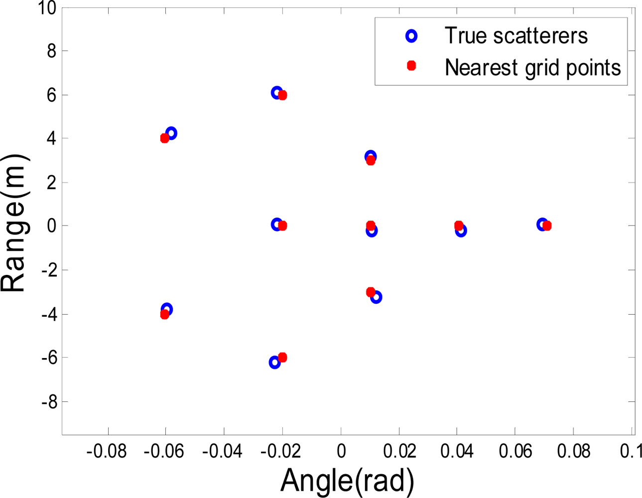
The original scatterer distribution of the target is shown in Figure 2. There are U = 40 radial range bins and V = 40 angle bins whose adjacent intervals are 0.5 m and 0.005 rad, respectively. And there are 10 scatterers with the unit reflection coefficient in the scene of interest. From Figure 2, we know that the scatterers of the scene are off the grid.

In the following simulations, besides SACR-iMAP, other algorithms will be involved: MF, OMP, FOCUSS, S-TLS [12] and TLS-FOCUSS [13]. S-TLS seeks to solve the following optimization problem:

$${\left\{{\widehat{\mathit{\sigma }}}^{\prime },\widehat{\mathit{\Lambda }}\mathit{r},\widehat{\mathit{\Lambda }}\mathit{\theta },\widehat{\xi }\right\}}_{\mathit{S-TLS}}=\underset{{\mathit{\sigma }}^{\prime },\mathit{\Lambda }\mathit{r},\mathit{\Lambda }\mathit{\theta },\xi }{\text{argmin}}\left\{\xi {\Vert {\mathit{\sigma }}^{\prime }\Vert }_1+{\Vert \mathit{z}-\left(\mathit{H}+\widehat{\mathit{H}}\mathit{\Lambda }\right){\mathit{\sigma }}^{\prime }\Vert }_2^2+{\Vert \mathit{\Lambda }\Vert }_2^2\right\}$$

(34)

From the Bayesian perspective, S-TLS is equivalent to searching for the MAP solutions by assuming that the added noise is white Gaussian, σ′ is Laplacian and Λ is Gaussian.

Similarly, TLS-FOCUSS is equivalent to searching for the MAP solutions by assuming that the added noise is white Gaussian, σ′ is l_p-term forced and Λ is Gaussian.

$${\left\{{\widehat{\mathit{\sigma }}}^{\prime },\widehat{\mathit{\Lambda }}\mathit{r},\widehat{\mathit{\Lambda }}\mathit{\theta },\widehat{\xi }\right\}}_{\mathit{TLS-FOCUSS}}=\underset{{\mathit{\sigma }}^{\prime },\mathit{\Lambda }\mathit{r},\mathit{\Lambda }\mathit{\theta },\xi }{\text{argmin}}\left\{\xi {\Vert {\mathit{\sigma }}^{\prime }\Vert }_p^p+{\Vert \mathit{z}-\left(\mathit{H}+\widehat{\mathit{H}}\mathit{\Lambda }\right){\mathit{\sigma }}^{\prime }\Vert }_2^2+{\Vert \mathit{\Lambda }\Vert }_2^2\right\}$$

(35)

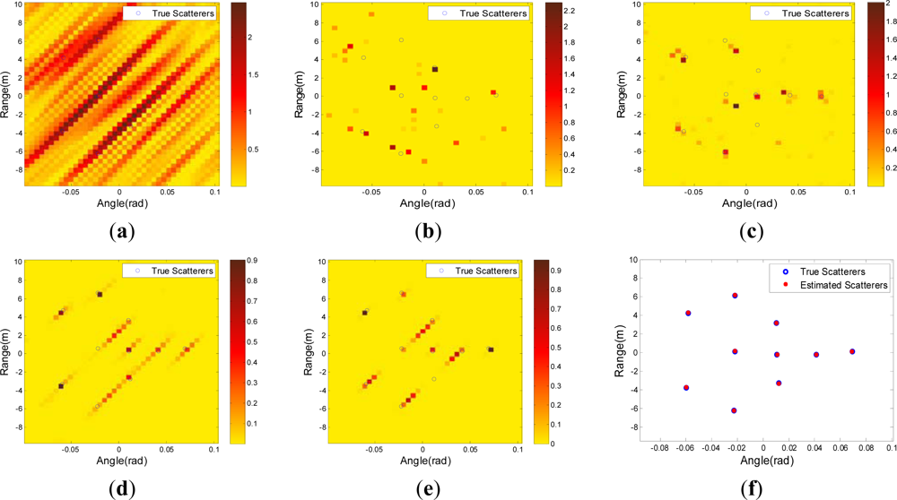
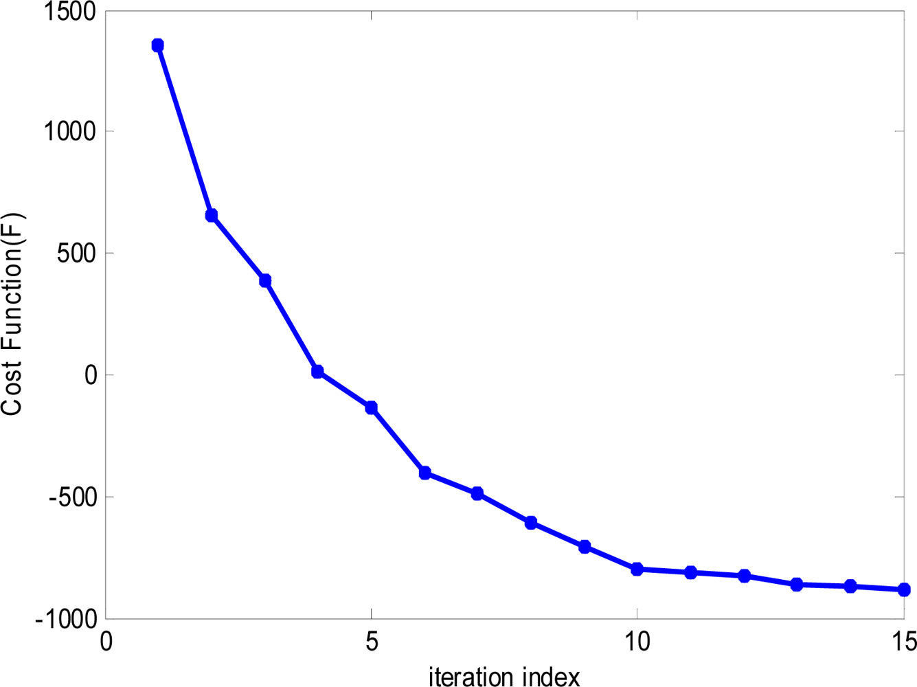
Figure 3(a–d) shows the imaging results by MF, OMP, FOCUSS, S-TLS, TLS-FOCUSS and our proposed method (SACR-iMAP), where the blue circles represent the true scatterers. As stated above, the imaging results by MF totally fail, because of the incomplete wavenumber-domain coverage. The OMP and FOCUSS methods are likely to fail, since the off-grid scatterers exist. Comparing with OMP and FOCUSS, S-TLS and TLS-FOCUSS can get improved recovery results. However, the off-grid errors cannot be calibrated accurately, so the imaging performance is not good. In contrast, our proposed method can deal with the off-grid scatterers, and thus, the imaging performance is good. Furthermore, as shown in Figure 4, during the whole imaging process, the cost function F keeps decreasing after each iteration, as proved in Remarks (2).

4.2. NMSE of the Imaging Results under Various SNR Conditions

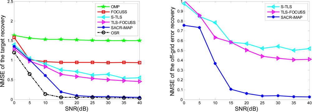
In this subsection, we study the imaging error with respect to the SNR level. The target recovery errors, as well as the off-grid recovery errors, are averaged over 30 trials. In each trial, the off-grid errors are uniformly distributed in the region of one radial range bin or angle bin. We use the same data as Section 4.1, and expect that the SNR varies from 0 dB to 40 dB with interval 5 dB.

Assuming that the off-grid errors are known a priori, then it can obtain the best imaging result, since it exploits the exact, oracle information of the off-grid errors. We name it as oracle sparse recovery (OSR) [25] for comparison with other approaches. The normalized mean square error (NMSE) of the target recovery results by OMP, FOCUSS, S-TLS, TLS-FOCUSS, SACR-iMAP and OSR versus SNR are shown in Figure 5. From Figure 5, it can be seen that by OMP and FOCUSS, the target recovery errors always maintain a high level, even when the SNR increases. Using S-TLS and TLS-FOCUSS, we can obtain improved recovery results to some extent. However, since the off-grid errors are uniformly distributed, the assumption about Λ in S-TLS and TLS-FOCUSS could not capture the property of Λ, so the target recovery and the off-grid error recovery results by S-TLS and TLS-FOCUSS are not good. However, SACR-iMAP can get a better target recovery and also off-grid recovery result when the SNR is greater than 15 dB. Expect the ideal case of OSR and SACR-iMAP has the smallest recovery error.

4.3. NMSE of the Imaging Results under Various Discretized Grid Intervals

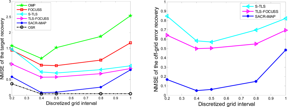
In this subsection, we assume that the size of the imaging area and the actual scatterer distribution of the target are invariant, then we change the discretized grid interval and, consequently, the number of the discretized radial range bins and angle bins. We assign SNR = 20 dB, and the target recovery errors, as well as the off-grid recovery errors, are averaged over 30 trials.

Figure 6 presents the corresponding simulation results. When the grid interval is less than 0.4 (normalized by Res_r and Res_θ), the dense grid enhances the coherence between the column of the sensing matrix, which leads to the violation of the RIP condition for reliable sparse recovery. From Figure 6, when the grid interval is 0.2, OMP, FOCUSS, S-TLS, TLS-FOCUSS, SACR-iMAP and OSR, all have different levels of performance deterioration. When the interval is greater than 0.4 (normalized by Res_r and Res_θ), a nearly constant NMSE is obtained using OSR, since the off-grid errors are assumed to be known exactly. The errors of OMP, FOCUSS, S-TLS and TLS-FOCUSS always maintain a high level with the discretized grid interval. Besides, the error of SACR-iMAP also increases with the discretized grid interval; however, the level of NMSE is lower than those of OMP and FOCUSS and apparently higher than that of OSR. When the interval is 1 (normalized by Res_r and Res_θ), the SACR-iMAP fails to improve the recovery performance, because a larger interval leads to higher approximation errors due to high order terms of Taylor expansion. Such a behavior is consistent with our analysis.

5. Conclusions

This paper presents the SACR-iMAP method to realize high resolution imaging of sparse, but off-grid, targets for the FD-MIMO radar system. Unlike traditional sparse recovery methods, SACR-iMAP adaptively adjusts the off-grid errors, meanwhile seeking the optimal target reconstruction result. Through iterative MAP, it turns the non-convex optimization problem of off-grid sparse recovery to three main stages: sparse recovery, off-grid errors calibration and parameter update. Benefited from adaptively adjusting and updating, SACR-iMAP has some merits, e.g., there is no need for accurate initialization and improved robustness to noise. The derivations and numerical simulations illustrate the effectiveness of the new method, which shows the potential for the method to be applied in practical systems.

In this paper, we only consider the case of FD-MIMO radar imaging; however, the framework in this paper can be extended to other imaging radar systems, such as generalized MIMO radar imaging and passive radar imaging, so SACR-iMAP will have wider applications. Here, we only consider the first order Taylor approximation of the off-grid errors. Higher order approximations can be adopted in the future to further reduce the modeling error and, hence, to achieve higher precision. Moreover, in the off-grid problem formulation, the scatterers and off-grid errors are jointly sparse. Inspired by the recent works on block and structured sparsity [26–28], our future work is to fully excavate the joint sparsity to accelerate the convergence of SACR-iMAP and, meanwhile, improve the recovery performance.

References

- Fishler, E.; Haimovich, A.; Blum, R.; Chizhik, D.; Cimini, L.; Valenzuela, R. MIMO Radar: An Idea Whose Time Has Come. Proceedings of IEEE Radar Conference, Boston, MA, USA, 17– 20 April 2007; pp. 71–78.
- Dai, X.Z.; Xu, J.; Peng, Y.N. High Resolution Frequency MIMO Radar. Proceedings of IEEE Radar Conference, Boston, MA, USA, 17– 20 April 2007; pp. 693–698.
- Zhang, J.J.; Suppappola, A.P. MIMO Radar with Frequency Diversity. Proceedings of International Waveform Diversity Design (WDD), Orlando, FL, USA, 8–13 February 2009; pp. 208–212.
- Liu, C.C.; Chen, W.D. Sparse Frequency Diverse MIMO Radar Imaging. Proceedings of the 46th Asilomar Conference on Signals, Systems, and Computers, Pacific Grove, CA, USA, 4–7 November 2012.
- Wang, W.Q. Space-time coding MIMO-OFDM SAR for high-resolution imaging. IEEE Trans. Geosci. Remote Sens 2011, 49, 1–11. [Google Scholar]
- Chen, C.Y.; Vaidyanathan, P.P. Compressive Sensing in MIMO Radar. Proceedings of 42nd Asilomar Conference on Signals, Systems and Computers, Pacific Grove, CA, USA, 26–29 October 2008; pp. 41–44.
- Yu, Y.; Petropulu, A.P.; Poor, H.V. CSSF MIMO radar: Low-complexity compressive sensing based MIMO radar that uses step frequency. IEEE Trans. Aerosp. Electron. Syst 2012, 48, 1490–1504. [Google Scholar]
- Tan, X.; Roberts, W.; Li, J.; Stoica, P. Sparse learning via iterative minimization with application to MIMO radar imaging. IEEE Trans. Signal Process 2011, 59, 1088–1101. [Google Scholar]
- Zhang, L.; Xing, M.; Qiu, C.; Li, J.; Bao, Z. Achieving higher resolution ISAR imaging with limited pulses via compressive sampling. IEEE Geosci. Remote Sens. Lett 2009, 6, 567–571. [Google Scholar]
- Gleichman, S.; Eldar, Y. Blind compressed sensing. IEEE Trans. Inform. Theory 2011, 57, 6958–6975. [Google Scholar]
- Chi, Y.; Scharf, L.; Pezeshki, A.; Calderbank, A. Sensitivity to basis mismatch in compressed sensing. IEEE Trans. Signal Process 2011, 59, 2182–2195. [Google Scholar]
- Zhu, H.; Leus, G.; Giannakis, G. Sparsity-cognizant total least-squares for perturbed compressive sampling. IEEE Trans. Signal Process 2011, 59, 2002–2016. [Google Scholar]
- Han, X.B.; Zhang, H.; Li, G. Fast Algorithms for Sparse Recovery with Perturbed Dictionary, Available online: http://arxiv.org/abs/1111.6237 (accessed on 1 May 2012).
- Yang, Z.; Xie, L.; Zhang, C. Off-Grid Direction of Arrival Estimation Using Sparse Bayesian Inference, Available online: http://arxiv.org/abs/1108.5838 (accessed on 17 September 2012).
- Ji, S.; Xue, Y.; Carin, L. Bayesian compressive sensing. IEEE Trans. Signal Process 2008, 56, 2346–2356. [Google Scholar]
- Huang, T.; Liu, Y.; Meng, H.; Wang, X. Adaptive matching pursuit with constrained total least squares. EURASIP J. Adv. Signal Process 2012. [Google Scholar] [CrossRef]
- Tang, G.; Bhaskar, B.N.; Shah, P.; Recht, B. Compressed Sensing off the Grid, Available online: http://arxiv.org/abs/1207.6053 (accessed on 25 July 2012).
- Fannjiang, A.; Tseng, H. Compressive Radar with Off-Grid and Extended Targets, Available online: http://arxiv.org/abs/1209.6399 (accessed on 28 September 2012).
- Carrara, W.G.; Goodman, R.S.; Majewski, R.M. Spotlight Synthetic Aperture Radar-Signal Processing Algorithm; Artech House: Norwood, MA, USA, 1995. [Google Scholar]
- Liu, C.C.; Xu, H.; He, X.Z.; Chen, W.D. The Distributed Passive Radar 3-D Imaging and Analysis in Wavenumber Domain. Proceedings of IEEE International Conference on Signal Processing (ICSP), Beijing, China, 24– 28 October 2010; pp. 2051–2054.
- Wipf, D.P.; Rao, B.D. Sparse bayesian learning for basis selection. IEEE Trans. Signal Process 2004, 52, 2153–2164. [Google Scholar]
- Gorodnitsky, I.F.; Rao, B.D. Sparse signal reconstructions from limited data using FOCUSS: A re-weighted minimum norm algorithm. IEEE Trans. Signal Process 1997, 45, 600–616. [Google Scholar]
- Franklin, J.N. Matrix Theory; Dover Publications: Dover, UK, 2000. [Google Scholar]
- CVX Research Inc. CVX: Matlab Software for Disciplined Convex Programming, Version 2.0 Beta. Available online: http://cvxr.com/cvx (accessed on 4 September 2012).
- Yang, Z.; Zhang, C.; Xie, L. Robustly Stable Signal Recovery in Compressed Sensing with Structured Matrix Perturbation, Available online: http://arxiv.org/abs/1112.0071 (accessed on 14 March 2012).
- Zheng, J.; Kaveh, M. Direction-of-Arrival Estimation Using A Sparse Spatial Spectrum Model with Uncertainty. Proceedings of IEEE International Conference on Acoustics, Speech and Signal Processing (ICASSP), Prague, Czech Republic, 22– 27 May 2011; pp. 2848–2551.
- Eldar, Y.; Kuppinger, P.; Bolcskei, H. Block-sparse signals: Uncertainty relations and efficient recovery. IEEE Trans. Signal Process 2010, 58, 3042–3054. [Google Scholar]
- Bach, F.; Jenatton, R.; Mairal, J.; Obozinski, G. Structured Sparsity through Convex Optimization, Available online: http://arxiv.org/abs/1109.2397 (accessed on 20 April 2012).
Appendix
Proof of Remark (2)
Proof: It is equivalent to prove that the cost function F of SACR-iMAP decreases in each of the three stages: sparse recovery, off-grid errors calibration and parameter update. Firstly, in the sparse recovery stage, Λ(l) and ξ(l) are kept unchanged. We write F = F1 + R1, where R1 is independent of σ′. The difference between F1(σ′(l+1)) and F1(σ′(l)) totally reflects the change of F. Furthermore, since there exists an internal iteration, we have to consider F1(σ′(l,s+1)) in the (s+1)-th internal step, i.e., we have to compare between F1(σ′(l,s+1)) and F1(σ′(l,s)). It is showed in [21] that F1(σ′(l,s+1)) is smaller than F1(σ′(l,s)) based on the fact that f(y) = yq (y > 0, 0 < q < 1) have the concave property. Therefore, the cost function keeps decreasing till the internal iteration converges, yielding σ′(l+1). So, there is no doubt that F1(σ′(l+1)) < F1(σ′(l)) as σ′(l) and σ′(l+1) represent the initial value and the converged value of the internal iteration, respectively. Therefore, we prove that F1, i.e., F decreases after the sparse recovery stage.
Secondly, in the off-grid errors calibration stage, similarly, we rewrite F = F2 + R2, where R2 is independent of Λ. Equation (28) is equivalent to Equation (30), so we have F2(Λ(l+1)) = F2(Δ(l+1)) and F2(Λ(l)) = F2(Δ(l)). Furthermore, we can deduce that:
Finally, since the parameter ξ(l+1) is computed according to ∂F/∂ξ(l+1) = 0, it would definitely result in the decrease of the cost function F after the parameter update stage.
Based on all the analysis above, we know that the cost function F of SACR-iMAP decreases in each stage of the (l+1)-th iteration. Therefore, It can be proved that F decreases with the iteration index l.