Area-Based Mapping of Defoliation of Scots Pine Stands Using Airborne Scanning LiDAR

 ,
, 
Abstract
: The mapping of changes in the distribution of insect-caused forest damage remains an important forest monitoring application and challenge. Efficient and accurate methods are required for mapping and monitoring changes in insect defoliation to inform forest management and reporting activities. In this research, we develop and evaluate a LiDAR-driven (Light Detection And Ranging) approach for mapping defoliation caused by the Common pine sawfly (Diprion pini L.). Our method requires plot-level training data and airborne scanning LiDAR data. The approach is predicated on a forest canopy mask created by detecting forest canopy cover using LiDAR. The LiDAR returns that are reflected from the canopy (that is, returns > half of maximum plot tree height) are used in the prediction of the defoliation. Predictions of defoliation are made at plot-level, which enables a direct integration of the method to operational forest management planning while also providing additional value-added from inventory-focused LiDAR datasets. In addition to the method development, we evaluated the prediction accuracy and investigated the required pulse density for operational LiDAR-based mapping of defoliation. Our method proved to be suitable for the mapping of defoliated stands, resulting in an overall mapping accuracy of 84.3% and a Cohen’s kappa coefficient of 0.68.1. Introduction
Evergreen coniferous forests dominate the landscapes in Finland, covering approximately 76% of the national land base. As such, forests have importance across economic, environmental, and societal domains. Chiefly through settlement and management activities these forests have been altered by humans, with most of the natural mature forests having been replaced with younger, even-aged managed forests. As a northern nation, climate change and related effects are considered to be among the most serious environmental issues threatening the health of forests in Finland. Average annual temperatures have increased more in northern latitudes than the global mean rise [1]. Furthermore, it has been found that changes in climate and related increased frequency of extreme weather events are altering the ecological balance of forests, [2] causing widespread damages by insects pest in managed forests [3]. The Mountain pine beetle (Dendroctonus ponderosae Hopkins) (Coleoptera: Scolytidae) in Canada provides an additional example, where cold winter temperatures historically served to limit the extent of the insect within a larger extent of possible hosts. Changes in climate have resulted in an alteration to the temperature regime, resulting in the spread of Mountain Pine Beetles into previously un-infested regions [4]. Spatial change in the nature of insect-related forest disturbances have also been noted, with disturbance events now observed to cover larger areas than previously experienced (e.g., [5]). Similar to the disturbance area and spread into new, previously un-infested, environments of bark beetles in North America [4,6], outbreaks of defoliating insects and bark beetles have increased rapidly in the past two decades in northern Europe [7–11].
Development of modern, cost-effective, mapping and monitoring methods for forest sites affected by climate-driven disturbance agents is urgently needed [12,13]. Typically the mapping, and often also the monitoring, of defoliation has been based on field sampling [14]. Field sampling is generally seen as costly, and in the case of capturing defoliation, it may often produce biased results. Field sampling of defoliation can be biased due to an array of spatial and temporal considerations, whereby defoliation events may be missed because of issues including location, timing of defoliation in relation to field visits, access, and number of plots allocated. Furthermore, as defoliation does not typically result in mortality, the impacts of a given event are indicative of longer-term impacts, such as a reduced yield expectation over a given period of time [5,15]. Based on particular site conditions, the accrual of fiber follows a known trajectory (yield), and the loss of photosynthetic activity through the defoliation reduces the expected longer term yield. This long-term loss in yield alters volume predictions from a forest management perspective, resulting in a need to revisit harvest scheduling and total fiber volume levels present over a given woodshed. Inventory-based estimates of volume are often statistically linked to biomass to produce modeled estimates of carbon that, in turn, can be used to inform on the exchange of gases between terrestrial ecosystems and the atmosphere (e.g., [16]). As such, capturing factors that perturb the capacity to accumulate fiber, such as defoliation, is increasingly important. The Finnish Forest Institute carries out the National Forest Inventory (NFI) [17], through which information on forest health is collected and monitored on a strategic level. While useful for some purposes, more precise (spatial, temporal, and categorical) information on forest disturbances is required to meet the current and growing needs of forest health monitoring.
Remote sensing is an increasingly established source of data to support mapping and monitoring of forested areas, including aspects related to condition, structure, and dynamics [18,19]. The capacity of remote sensing to characterize forests has been furthered by the advent of airborne scanning LiDAR (Light Detection And Ranging) technology and related information extraction techniques [20]. With the capability of direct or derived measurement of three-dimensional (3D) forest structure—including canopy height [21], crown dimensions [22], and biomass [23]—LiDAR can also be applied to the monitoring of various forest disturbances [7,8,24,25]. In Nordic countries, scanning LiDAR is already applied to many practical applications, including the creation of accurate digital terrain models (DTMs), urban engineering, and forest management planning [26]. In operational forest management planning, a two-stage procedure using LiDAR and field plots, an area-based approach (ABA, [27]), has become common and a reference against which other inventory methodologies are compared. The foremost advantages of the state-of-the-art LiDAR ABA compared with traditional stand-wise field inventory (SWFI) include more precise prediction of forest variables and sample-based estimation with the capacity for the calculation of accuracy statistics, and, at least in principle, LiDAR-based inventory does not require delineation of stand boundaries. Although current LiDAR data acquisition and processing costs are lower than that of traditional SWFI methods in Finland, expansion of the possible uses of LiDAR data in a forest management and monitoring context further justifies the expenditure. Additional applications using LiDAR data to capitalize upon the unique information content are incremental, offering an opportunity to supplement inventory data bases. Forest health status and dynamics are an example where an information deficit exists that could also be addressed by LiDAR.
The capability of scanning LiDAR in mapping of defoliation has been demonstrated for a pine sawfly attack in Norway [7]. LiDAR was acquired both before and after the insect attack, and the defoliation was derived from the change in penetration rate and Leaf Area Index (LAI). Other studies have posited that defoliation may be detected without having repeated ALS acquisitions, and that different types of disturbances can be distinguished based on the type of ALS penetration through the forest canopy [10]. Kantola et al.[8] tested the classification of defoliated and healthy trees using a survey configured for high density LiDAR data acquisition (20 pulses/m2) in conjunction with aerial images. The classification accuracies ranged between 83.7% and 88.1% (kappa value 0.67–0.76) depending on the classification method applied. It should be noted that the trees used in the classification were clearly divided into healthy and defoliated trees, thus the results are not applicable in an operational setting. However, the study proved that defoliated and healthy trees produce statistically separable point clouds and that the application showed potential and was worthy of further study.
The aim of this study was to develop and evaluate a LiDAR-based method for mapping defoliation caused by the Common pine sawfly (Diprion pini L.) (Hymenoptera: Diprionidae). Implementation of this method requires plot-level training data regarding defoliation and co-located LiDAR data. Our hypothesis is that in defoliated stands, a greater proportion of LiDAR pulses will penetrate more deeply into the forest canopy. We tested this hypothesis for an inventory and management relevant two-class classification scheme. The difference in penetration noted was used to inform on defoliation. The classes are separated using a threshold. Our predictions were made at the plot-level, which enables direct linking the method to the operational forest management planning. In addition to the method development, we evaluated the prediction accuracy and investigated the impact of pulse density for the LiDAR-based mapping of defoliation.
2. Materials
2.1. Study Area
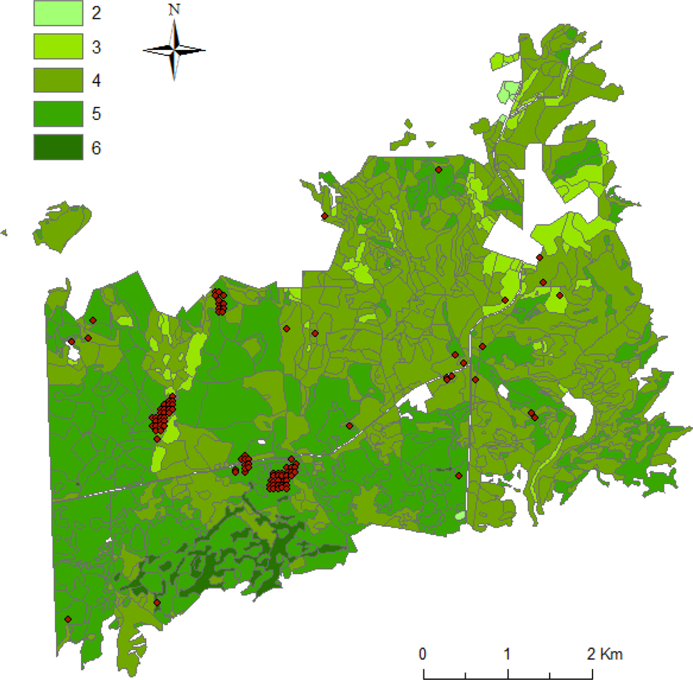
The field work for this research was carried out over a 34.5 km2 area in the Palokangas area, Ilomantsi, found in the eastern corner of Finland (62°53′N, 30°54′E, Figure 1). Dry to dryish forest site types dominate the region. Forests of the study area are dominated (at 99.5%) by Scots pine (Pinus sylvestris L.) (Pinaceae). The majority of the stands are young to middle-aged, having a mean age of 53 years and a mean diameter of 14.7 cm. The initial outbreak of D. pini initiated on the western coast of Finland in 1997, impacted over 500,000 ha in central Finland, and became apparent in 1999 in the Palokangas area. Since then, the outbreak range in Palokangas has fluctuated spatially between 10,000 and 15,000 ha. Both population density and damage intensity have varied on an annual basis in recent years. Severe infestation over successive years led to mortality being observed 2006–2008.
The field measurements were carried out in May and early June 2009 before the elongation of current needles, representing the defoliation status of the fall of 2008. A total of 106 plots (r = 8 m, Table 1), growing in mainly pure mature and maturing Scots pine forest stands, were inventoried using adaptive cluster sampling (ACS) as a sampling method (see more details in [28]). Following ACS, an initial set of units is selected using a probability sampling procedure and additional units from the neighborhood are added [28]. The procedure is iterative and is repeated until no additional units satisfy the required criteria (in our case, presence of plot-wise defoliation). According to (e.g., [28–30]), ACS has advantages over more conventional sampling methods, especially in sampling rare and clustered phenomena through focusing of sampling efforts on areas well represented by the variable of interest.
The sample plot centers were positioned with a Trimble Pro XH (Trimble Navigation Ltd., Sunnyvale, California, USA), designed to reach 30 cm precision. Differential post processing was applied. Individual trees were also located and spatially recorded. The visual assessment of defoliation severity was performed simultaneously with tree- and stand-wise measurements, performed by experts with similar experience, following established defoliation categorization criteria. The defoliation severity of each tree was visually assessed from different directions, according to Eichhorn [31], comparing the amount of needles present to an imaginary reference tree with full healthy complement of foliage growing on the same site type in with the same canopy cover level. Intervals of 10% were used for the categorization of needle loss. The same procedure for needle loss assessment is utilized, for example, by the Finnish National Forest Inventory (NFI) [17]. The plot-wise defoliation levels were calculated as an average of the needle losses of the trees found in the two dominant strata encompassing each plot. The defoliation levels of the plots varied between 0% and 50%, and the tree-wise defoliation levels varied between 0% and 100%. Overall, the trees and the plots had on average 10% to 30% needle loss, respectively.
2.2. LiDAR Data
The LiDAR data was acquired in October 2008 with a Leica ALS50-II SN058 laser scanner (Leica Geosystem AG, Heerbrugg, Switzerland). The flying altitude was 500 m at a speed of 80 knots, with a field of view of 30 degrees, pulse rate of 150 kHz, scan rate of 52 Hz, and a ground footprint diameter of 0.11 m. The density of the LiDAR data was approximately 20 pulses/m2. LiDAR data were classified into ground or non-ground points using the standard TerraScan approach, as explained by Axelsson [32]. A digital terrain model was created using classified ground points. LiDAR heights above the ground (normalized height or canopy height) were calculated by subtracting the ground elevation from corresponding non-ground LiDAR measurements.
3. Methods
3.1. General Workflow
Mapping of the defoliated forest stands was based on a two-stage procedure using LiDAR and field plots. LiDAR returns that are reflected from the canopy were used to calculate features that were used in the needle loss prediction. Forest canopy cover (FCC) is known to effect the penetration of LiDAR pulses in a forested environment and thus, must be considered in the area-based predictions of defoliation. In this study, within plot FCC is first determined, with LiDAR features calculated only from that particular area (i.e., uses only the LiDAR returns that are reflected from within the forest canopy). Other factors hindering reliable defoliation prediction include overlapping branches from neighboring trees and understory vegetation. To minimize the effect of these factors, only LiDAR returns reflected above mean plot height are used. The mean height estimate is calculated as 50% of the maximum LiDAR height. Additionally, in the boreal forest environment of this study, tree crowns above this mean height designation typically do not overlap. In addition, with regards to understory vegetation or suppressed trees, such as understory spruces, are found below this level (although understory is only of slight concern in this study area due to the dominance of Scots pine). Basic steps in our method (with references to corresponding sections in this study) are as follows:
Measure plot-level ground truth about defoliation (Section 2.1)
Acquire LiDAR (Section 2.2)
Preprocess LiDAR (Section 2.2)
Determine operationally appropriate classification schemes for defoliation (Section 3.2)
Determine FCC from LiDAR (Section 3.3)
Calculate LiDAR features from canopy returns (Section 3.4)
Combine LiDAR features and plot-level ground truth (Section 3.4)
Predict defoliation at the plot-level (Section 3.5)
Map the area-wide defoliation and validate method at the plot-level (Section 4)
3.2. Classification Schemes for Defoliation Based on Expert Observations in the Field
The field plots were classified using two classes based on defoliation level. The threshold value of 20% of defoliation between healthy and defoliated stands was used. Defoliation above the level of 20% is understood by practitioners as the level of notable defoliation, at which a long-term reduction in yield is anticipated.
3.3. Determination of the Forest Canopy Cover Using LiDAR
FCC was mapped following delineation of tree crown surface area using individual tree detection (ITD) procedures. Using increasingly standard methods, consistent and reliable mapping is possible with operationally viable levels of detection accuracy [33–35]. Readers are recommended to refer to the original references for a detailed description of tree delineation in ITD [22,36,37]. Specifically using ITD as a means for FCC delineation is only briefly described here. The FCC delineation method used was based on the creation of a normalized surface model (nDSM, or in case of a forest, canopy height model, CHM), and then FCC was delineated using watershed segmentation from a smoothed nDSM (e.g., [22,36]). The threshold height used to delimit created FCC segments was 50% of the maximum LiDAR height of the plot.
3.4. Extraction of LiDAR Features from Canopy Returns
After FCC areas were segmented, the co-located LiDAR point clouds were extracted separately for each segment. LiDAR features describing height of the trees and density of the crowns were calculated. Features included maximum (Hmax), mean (Hmean), and standard deviation (Hstd) of LiDAR heights. In addition, proportions of canopy returns below various relative heights were calculated (Table 2). In the calculation of LiDAR features, we used “first” and “only” returns. The rationale for using only these returns is largely based upon the presence of many uncertainties in those returns coming after a pulse starts to penetrate into a tree canopy (i.e., is the pulse penetrated trough a tree that is not within the plot, overlapping crowns, and understory vegetation). To ensure a focus on the upper canopy and crowns, LiDAR returns with the height above ground being greater than the mean height of the plot (50% of Hmax) were used in the calculations. This mid-canopy stratification for each plot is unique compared to most other studies utilizing LiDAR in forest mapping. Calculated LiDAR metrics were finally linked to the plot-level ground measurements by using the GPS-measured plot locations.
3.5. Prediction of Defoliation Using Random Forest
A nearest neighbor (NN) approach was used in plot-wise needle loss prediction. Plot-level defoliation determined in the field was used as target observation (y value), and features calculated from LiDAR canopy returns were used as predictors (x values). Random Forest (RF, [38]) was applied in the search for nearest neighbors. The RF method is explained in detail by Crookston and Finley [39] as well as Falkowski et al.[40]. Hudak et al.[41] and Latifi et al.[42] showed that the RF method is robust and flexible in forest variable prediction compared with other NN methods. In the RF method, several regression or classification trees are generated by drawing a replacement of two-thirds of the data for training and one-third for testing each tree (i.e., out-of-the-bag samples). A regression tree is a sequence of rules that splits the feature space into partitions having values similar to the response variable. Measurement of nearness in RF is defined based on observations of the probability of ending up in the same terminal node in classification. The output is the percent increase in the misclassification rate as compared to the out-of-bag rate (with all variables intact). A relatively small number of target observations (n = 106) forced us to use a small number of nearest neighbors (k) and out-of-the bag samples in evaluation. The number of k was chosen to be three, based on previous knowledge. In general, stable results are obtained in forest variable predictions with k values between two and seven, though bias being smallest with k = 1. A total of 2000 regression trees were fitted in each RF run to gain more consistency. Randomness was also taken into account by running the RF method 50 times and the final result was the average of these runs. The R statistical computing environment [42] and yaImpute library [39] were applied in the RF predictions. The yaImpute library is tailored to nearest-neighbor forest attribute estimation and mapping.
The preliminary predictors were chosen based on previous studies (e.g., [7,8,10,44]), correlations, and preliminary modeling results (i.e., the predictors were chosen on the basis of biological plausibility as well as statistical significance).
3.6. Simulation of the Effect of Pulse Density
The instrument used and applied configuration settings produced a dense coverage of LiDAR data (20 pulses/m2), which enabled simulations to determine the any effects of a pulse density upon mapping of defoliation. As a starting point, the full density of the LiDAR data (20 pulses/m2) was used to the delineation of FCC and to select LiDAR features for predictions. (Noting that the effect of the point density upon ITD and related FCC were not current objectives). After delineation of the FCC and feature selection, the data was thinned randomly. Randomness was taken into account by simulating the thinning and the prediction process 50 times and using averages of these runs as final results. Point densities of 20, 18, 16, 14, 12, 10, 8, 6, 4, 2, 1 and 0.5 pulses/m2 were simulated and tested. In Finland, LiDAR data with 0.5 pulses/m2 is used in operational forest management planning inventory.
4. Results
4.1. Interaction between LiDAR and Defoliated Forest Canopy
A little under a half of all plots available in the study (43.9%) were representative of defoliated conditions. The weighted average of diameter, height, basal-area and volume were 18.9 cm, 15.1 m, 16.6 m2/ha, and 121.1 m3/ha for healthy plots, and the respective statistics for defoliated plots were 24.9 cm, 19.1 m, 11.4 m2/ha, and 96.8 m3/ha. LiDAR Hmean and Hmax mean values were 11.9 m and 17.3 m in healthy plots and 14.0 m and 19.3 m in defoliated plots. These initial findings based on the field data alone reveal that the forest structure differs between these two classes. Thus, classification had to be done carefully in order to classify the phenomena of interest (defoliation), and not result in a general separation of stand structural types. In order to do so, the classifying features should not correlate with tree size. Hmean and Hmax describe tree size whereas proportions of the LiDAR returns from the upper canopy (p60, p70, p80 and p90) are relative measures that are not directly correlated with tree size. These features are also identified as eligible as suitable classifiers for defoliation. The mean values of p60, p70, p80 and p90 varied significantly in Student’s t-test between two defoliation classes (p = 0.00). In healthy plots a larger number of LiDAR returns was reflected from the upper canopy.
4.2. Area-Based Mapping of Defoliation
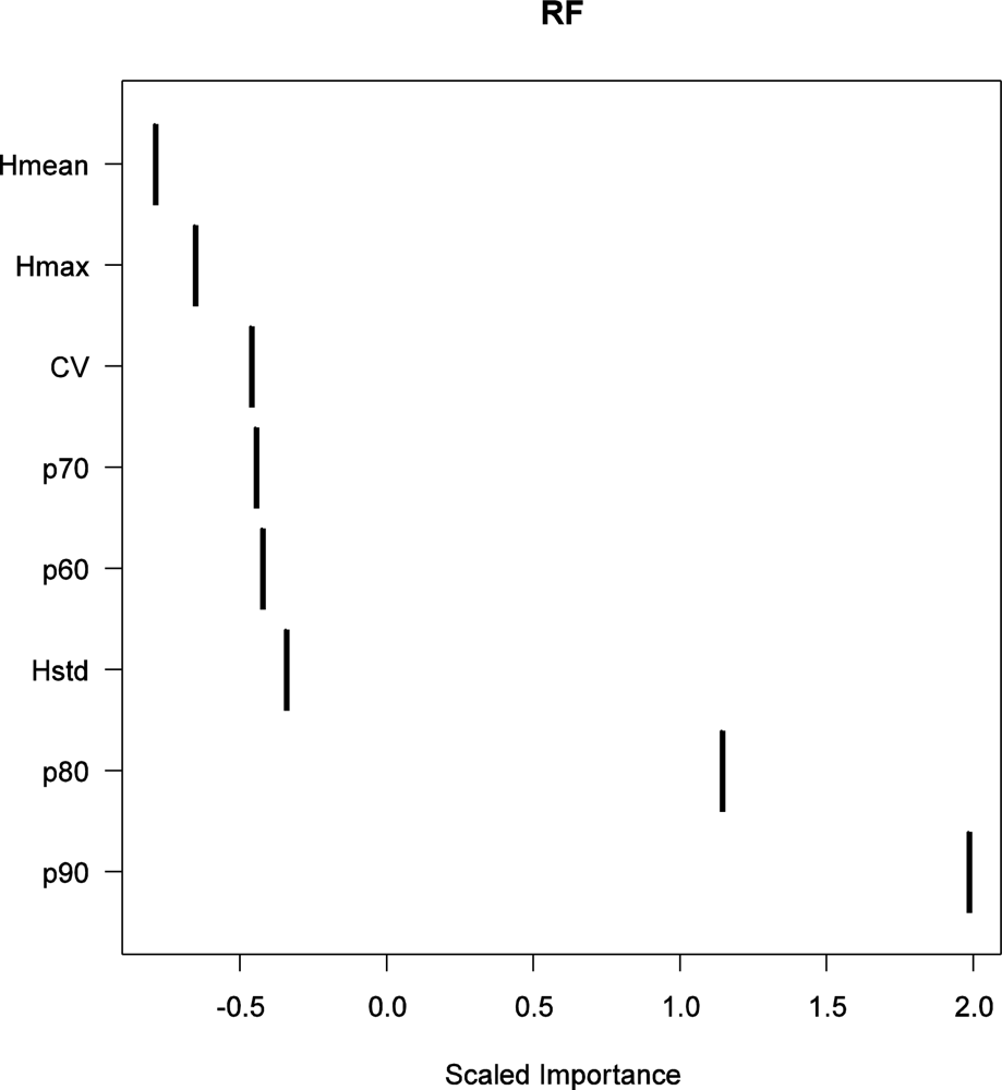
In the first phase, we implemented an RF run with all the possible classifiers included. This was justifiable as the overall number of classifiers was small (eight classifiers). Based on these RF runs, the most important classifiers were proportions of the upper-canopy LiDAR returns, p80 and p90 (Figure 2). Needle loss was then predicted using p80 and p90 as classifiers. Defoliated plots were classified with accuracy of 84.3% and a Cohen’s kappa coefficient (kappa) of 0.68.
4.3. Effect of Pulse Density to the Area-Based Mapping of Defoliation
Features p80 and p90 were used in the analyses of the effect of the LiDAR pulse density for mapping the defoliation. Simulated pulse densities varied between 0.5 and 20 pulses/m2. Features were calculated and the predictions made for 12 different pulse densities (Table 3, Figure 3). The mapping accuracy was not overly sensitive to LiDAR pulse density varying from 77.1% to 89.3%.
5. Discussion
In the next-generation forest management planning systems, it is anticipated that additional information on forest health will be required. Capture of forest health, and specifically defoliation, will allow for incorporation into management and planning variables that relate to growth loss and tree mortality. Thus, the forest management actions, such as which stands are to be harvested or subject to some silvicultural intervention, can be optimized differently than for healthy stands. The findings of this study present new information regarding how scanning LiDAR could be used in the mapping of defoliated stands. The hypothesis was that in defoliated stands, a larger proportion of the LiDAR returns should penetrate more deeply into the canopy. The results of the analyses supported our hypothesis. Although several LiDAR features were calculated for use as possible predictors, proportional penetration variables in the upper canopy were most informative. When using only two variables, mapping accuracy of 84.3% was obtained. Proportional LiDAR penetration variables are logical and straightforward, with the simple interpretation: With more intense needle loss, a greater proportion of LiDAR returns will be found in the lower canopy layers (when stratified by the half the maximum height at that location).
LiDAR sensors also collect information of pulse return intensity. LiDAR intensity is a measure of the spectral reflectance characteristics of the features that intercepting, and returning, the laser energy. In theory, based upon a wavelength of 1064 nm in the near-infrared, LiDAR return intensities should be lower in defoliated stands than in respective healthy stands. However, in practical applications, use of intensity is problematic because it must be calibrated. We made some classification tests using raw intensity information (i.e., we did not use any calibration) in addition to the p90 or p80. In a relatively small (in a practical sense) study area, it seemed that this was not causing a problem and intensity provided some additional explanatory power. Classification accuracy of 86.9% was obtained. Based on that test, it can also be assumed the LiDAR full waveform information could provide additional information regarding defoliation. The form of the waveform describes the interaction of the LiDAR pulse and forest canopy. Waveform information could be used in next-generation forest management planning system to map defoliation, instead of relying on intensity, if the calibration of the intensity causes practical problems. However, only a few studies exist in which full waveform LiDAR is used in the mapping of forests and the research remains in early stages.
Another practical problem in the mapping of defoliation relates to the field reference. Subjective estimation of the defoliation is a weakness. From the remote sensing point of view, another aspect to be aware of is that the defoliation classes are dependent on the site type (i.e., a tree or a stand that is 20% defoliated has more needles in a rich site than in a poor site type). Thus, mapping of the defoliation should always be stratified by site type. Fortunately, this information is often readily obtained, as it is also needed for other forest management purposes. We assume that the quality of site type information in this sense is not oversensitive. We did not stratify our data based on site type because the majority of the plots were located in similar site types.
We used ITD methods to estimate FCC that can also be considered as a forest canopy mask. FCC can be estimated also by simply thresholding the CHM, if that kind of delineation of the FCC, used in this study, seems to be computationally too intensive. We assume this should not affect the results significantly.
Our simulations with lower pulse densities are optimistic for two reasons: (1) We used dense data (20 pulses/m2) to delineate FCC, which was the basis for later analyses; and (2) this respective data set was used to select the optimal features to be used in the mapping of defoliation. However, we assume that this is not hampering our main finding, that our mapping method is not overly sensitive to the applied LiDAR pulse density.
The results of this study are, in some ways, comparable with other studies using remotely sensed data in needle loss prediction. Ilvesniemi [45] used the same Palokangas study area when investigating the usability of aerial photographs classifying plot-level defoliation. The classification accuracies varied between 38% (9 classes) and 87.3% (2 classes). Separate testing data was not used. Karjalainen et al.[9] used multitemporal ERS-2 and Envisat satellite images and calculated the SAR backscattering intensities of 400 m × 400 m grid cells to estimate defoliation. A classification accuracy of 67.8% for a test set (two classes) was obtained. Comparing our results to previous studies with other remote sensing instruments, scanning LiDAR appears to offer additional information. In area-based mapping of defoliation, the variation in FCC was seen as a major problem (i.e., [8,44]). In this study, we showed that the effect of FCC variation can be taken into account with a quite straightforward method. Area-based mapping methods are, however, more suitable than ITD based in practice. The results of the present study provide novel findings for mapping damage by pine sawflies and improving the inventory of disturbances by defoliators. Any new attributes generated, can be easily incorporated into the forest inventory database, providing additional information to inform planning and decision making. The scanning LiDAR-based approach for monitoring forest health is of especial interest as operational forestry is increasingly adapting LiDAR data into operational inventories. A capacity to characterize an expanded suite of attributes (such as defoliation) using the same LiDAR data—adding value to the inventory without an appreciable increase in costs—is demonstrated by this study.
6. Conclusions
In this study, an area-based method for the practical mapping of defoliation was developed and validated. Following this approach, it was possible to obtain 84.3% mapping accuracy for two operationally important defoliation classes by using proportions of canopy returns below 80% and 90% relative heights. We also found that the mapping accuracy was not overly sensitive to LiDAR pulse density. The method and information outcomes could be linked to operational forest management planning practices.
Acknowledgments
This study was made possible through financial aid from the Maj and Tor Nessling Foundation, Foresters Foundation, Niemi Foundation, Graduate School in Forest Sciences (GSForest), RYM Oy (program “Energizing Urban Ecosystems” WP3—Regional Innovation Ecosystems (RIE)) and the Academy of Finland (projects “Towards Precision Forestry” and “Intelligent Roadside Modeling”). We also wish to thank Tornator Ltd. for its kind co-operation.
References
- Soja, A.J.; Tchebakova, N.M.; French, N.H.F.; Flannigan, M.D.; Shugart, H.H.; Stocks, B.J.; Sukhinin, A.I.; Parfenova, E.I.; Chapin, F.S., III.; Stackhouse, P.W., Jr. Climate-induced boreal forest change: Predictions vs. current observations. Glob. Planet. Change 2007, 56, 274–296. [Google Scholar]
- Tkacz, B.; Moody, B.; Castillo, J.V.; Fenn, M.E. Forest health conditions in North America. Environ. Pollution 2008, 155, 409–425. [Google Scholar]
- Moore, B.; Allard, G. Climate Change Impacts on Forest Health; Forest Health and Biosecurity Working Paper FBS/34E; FAO: Rome, Italy, 2008. [Google Scholar]
- Safranyik, L.; Carroll, A.L.; Régnière, J.; Langor, D.W.; Riel, W.G.; Shore, T.L.; Peter, B.; Cooke, B.J.; Nealis, V.G.; Taylor, S.W. Potential for range expansion of mountain pine beetle into the boreal forest of North America. Canad. Entomol 2010, 142, 415–442. [Google Scholar]
- Lyytikäinen-Saarenmaa, P.; Tomppo, E. Impact of sawfly defoliation on growth of Scots pine Pinus sylvestris (Pinaceae) and associated economic losses. Bull. Entomol. Res 2002, 92, 137–140. [Google Scholar]
- Wulder, M.A.; White, J.C.; Grills, D.; Nelson, T.; Coops, N.C.; Ebata, T. Aerial overview survey of the mountain pine beetle epidemic in British Columbia: Communication of impacts. BC J. Ecosyst. Manag 2009, 10, 45–58. [Google Scholar]
- Sohlberg, S.; Næsset, E.; Hanssen, K.H.; Christiansen, E. Mapping defoliation during a severe insect attack on Scots pine using airborne laser scanning. Remote Sens. Environ 2006, 102, 364–376. [Google Scholar]
- Kantola, T.; Vastaranta, M.; Yu, X.; Lyytikäinen-Saarenmaa, P.; Holopainen, M.; Talvitie, M.; Kaasalainen, S.; Solberg, S.; Hyyppä, J. Classification of defoliated trees using tree-level airborne laser scanning data combined with aerial images. Remote Sens 2010, 2, 2665–2679. [Google Scholar]
- Karjalainen, M.; Kaasalainen, S.; Hyyppä, J.; Holopainen, M.; Lyytikäinen-Saarenmaa, P.; Krooks, A.; Jaakkola, A. SAR Satellite Images and Terrestrial Laser Scanning in Forest Damages Mapping in Finland. Proceedings of ESA Living Planet Symposium, Bergen, Norway, 28 June–2 July 2010. SP-686..
- Solberg, S. Mapping gap fraction, LAI and defoliation using various ALS penetration variables. Int. J. Remote Sens 2010, 31, 1227–1244. [Google Scholar]
- Jönsson, A.M.; Appelberg, G.; Harding, S.; Bärring, L. Spatio-temporal impact of climate change in the activity and voltinism of the spruce bark beetle, Ips. typographus. Glob. Change Biol 2009, 15, 486–499. [Google Scholar]
- Lyytikäinen-Saarenmaa, P.; Holopainen, M.; Ilvesniemi, S.; Haapanen, R. Detecting pine sawfly defoliation by means of remote sensing and GIS. Forstschutz Aktuell 2008, 44, 14–15. [Google Scholar]
- Wulder, M.A.; Ortlepp, S.M.; White, J.C.; Coops, N.C.; Coggins, S.B. Monitoring tree-level insect population dynamics with multi-scale and multi-source remote sensing. Spat. Sci 2008, 53, 49–61. [Google Scholar]
- Juutinen, P.; Varama, M. Ruskean mäntypistiäisen (Neodiprion sertifer) esiintyminen Suomessa vuosina 1966–83. Folia Forestalia 1986, 662, 1–39. [Google Scholar]
- Lyytikäinen-Saarenmaa, P.; Niemelä, P.; Annila, E. Growth Responses and Mortality of Scots Pine (Pinus sylvestris L.) after a Pine Sawfly Outbreak. Proceedings of the International Symposium of IUFRO “Forest Insect Population Dynamics and Host Influences”, Kanazawa, Japan, 14–19 September 2003; pp. 81–85.
- Metsaranta, J.M.; Kurz, W.A.; Neilson, E.T.; Stinson, G. Implications of future disturbance regimes on the carbon balance of Canada’s managed forest (2010–2100). Tellus 2010, 62, 719–728. [Google Scholar]
- Tomppo, E. The Finnish National Forest Inventory. In Forest Inventory. Methodology and Applications (Managing Forest Ecosystems); Kangas, A., Maltamo, M., Eds.; Springer: Dordrecht, The Netherlands, 2006; pp. 179–194. [Google Scholar]
- Hall, R.J.; Skakun, R.S.; Arsenault, E.J. Remotely Sensed Data in the Mapping of Insect Defoliation. In Understanding Forest Disturbance and Spatial Pattern. Remote Sensing and GIS Approaches; Wulder, M.A., Franklin, S.E., Eds.; CRC Press, Taylor & Francis Group: Boca Raton, FL, USA, 2007; pp. 85–111. [Google Scholar]
- Wulder, M.A. Optical remote sensing techniques for the assessment of forest inventory and biophysical parameters. Progr. Phys. Geogr 1998, 22, 449–476. [Google Scholar]
- Hyyppa, J.; Hyyppa, H.; Leckie, D.; Gougeon, F.; Yu, X.; Maltamo, M. Review of methods of small-footprint airborne laser scanning for extracting forest inventory data in boreal forests. Int. J. Remote Sens 2008, 29, 1339–1366. [Google Scholar]
- Næsset, E. Determination of mean tree height of forest stands using airborne laser scanner data. ISPRS J. Photogramm 1997, 52, 49–56. [Google Scholar]
- Hyyppä, J.; Inkinen, M. Detecting and estimating attributes for single trees using laser scanner. Photogramm. J. Fin 1999, 16, 27–42. [Google Scholar]
- Koch, B. Status and future of laser scanning, synthetic aperture radar and hyperspectral remote sensing data for forest biomass assessment. ISPRS J. Photogramm 2010, 65, 581–590. [Google Scholar]
- Vastaranta, M.; Korpela, I.; Uotila, M.; Hovi, A.; Holopainen, M. Area-Based Snow Damage Classification of Forest Canopies Using Bi-Temporal Lidar Data. Proceedings of ISPRS Workshop on Laser Scanning 2011, Calgary, AB, Canada, 29–31 August 2011; p. 5.
- Vastaranta, M.; Korpela, I.; Uotila, A.; Hovi, A.; Holopainen, M. Mapping of snow-damaged trees in bi-temporal airborne LiDAR data. Eur. J. For. Res 2012, 131, 1217–1228. [Google Scholar]
- Næsset, E.; Gobakken, T.; Holmgren, J.; Hyyppä, H.; Hyyppä, J.; Maltamo, M.; Nilsson, M.; Olsson, H.; Persson, Å.; Söderman, U. Laser scanning of forest resources: The Nordic experience. Scand. J. For. Res 2004, 19, 482–499. [Google Scholar]
- Næsset, E. Predicting forest stand characteristics with airborne scanning laser using a practical two-stage procedure and field data. Remote Sens. Environ 2002, 80, 88–99. [Google Scholar]
- Talvitie, M.; Kantola, T.; Holopainen, M.; Lyytikainen-Saarenmaa, P. Adaptive cluster sampling in inventorying forest damage by the common pine sawfly (Diprion pini). J. For. Plan 2011, 16, 141–148. [Google Scholar]
- Thompson, S.K. Adaptive cluster sampling. J. Am. Statist. Assoc. 1990, 85. [Google Scholar]
- Roesch, F.A., Jr. Adaptive cluster sampling for forest inventories. For. Sci 1993, 39, 655–669. [Google Scholar]
- Eichhorn, J. Manual on Methods and Criteria for Harmonized Sampling, Assessment, Monitoring and Analysis of the Effects of Air Pollution on Forests. Part. II. Visual Assessment of Crown Condition and Submanual on Visual Assessment of Crown Condition on Intensive Monitoring Plots; United Nations Economic Commission for Europe Convention on Long-range Transboundary Air Pollution: Hamburg, Germany, 1998. [Google Scholar]
- Axelsson, P. DEM Generation from Laser Scanner Data Using Adaptive TIN Models. Proceedings of XIX ISPRS Congress, Commission I–VII, Amsterdam, The Netherlands, 16–23 July 2000; pp. 110–117.
- Vastaranta, M.; Holopainen, M.; Yu, X.; Hyyppä, J.; Mäkinen, A.; Rasinmäki, J.; Melkas, T.; Kaartinen, H.; Hyyppä, H. Effects of individual tree detection error sources on forest management planning calculations. Remote Sens. 2011, 3, 1614–1626. [Google Scholar]
- Vauhkonen, J.; Ene, L.; Gupta, S.; Heinzel, J.; Holmgren, J.; Pitkänen, J.; Solberg, S.; Wang, Y.; Weinacker, H.; Hauglin, K.M.; et al. Comparative testing of single-tree detection algorithms under different types of forest. Forestry 2012, 85, 27–40. [Google Scholar]
- Kaartinen, H.; Hyyppä, J.; Yu, X.; Vastaranta, M.; Hyyppä, H.; Kukko, A.; Holopainen, M.; Heipke, C.; Hirschmugl, M.; Morsdorf, F.; et al. An international comparison of individual tree detection and extraction using airborne laser scanning. Remote Sens 2012, 4, 950–974. [Google Scholar]
- Persson, Å.; Holmgren, J.; Söderman, U. Detecting and measuring individual trees using an airborne laser scanner. Photogramm. Eng. Remote Sensing 2002, 68, 925–932. [Google Scholar]
- Yu, X.; Hyyppä, J.; Vastaranta, M.; Holopainen, M. Predicting individual tree attributes from airborne laser point clouds based on random forest technique. ISPRS J. Photogramm 2011, 66, 28–37. [Google Scholar]
- Breiman, L. Random forests. Mach. Learn 2001, 45, 5–32. [Google Scholar]
- Crookston, N.L.; Finley, A.O. yaImpute: A R package for efficient nearest neighbor imputation routines variance estimation, and mapping, 2007–2010. Available online: http://cran.r-project.org (accessed on 18 October 2012).
- Falkowski, M.; Hudak, A.; Crookston, N.; Gessler, P.; Smith, A. Landscape-scale parameterization of a tree-level forest growth model: A k-NN imputation approach incorporating LiDAR data. Can. J. For. Res 2010, 40, 184–199. [Google Scholar]
- Hudak, A.; Crookston, N.; Evans, J.; Hall, D.; Falkowski, M. Nearest neighbor imputation of species-level, plot-scale forest structure attributes from LiDAR data. Remote Sens. Environ 2008, 112, 2232–2245. [Google Scholar]
- Latifi, H.; Nothdurft, A.; Koch, B. Non-parametric prediction and mapping of standing timber volume and biomass in a temperate forest: application of multiple optical/LiDAR-derived predictors. Forestry 2010, 83, 395–407. [Google Scholar]
- The R Project for Statistical Computing. Available online: http://www.r-project.org/ (accessed on 13 December 2012).
- Kantola, T.; Lyytikäinen-Saarenmaa, P.; Vastaranta, M.; Kankare, V.; Yu, X.; Holopainen, M.; Talvitie, M.; Solberg, S.; Puolakka, P.; Hyyppä, J. Using High Density ALS Data in Plot Level Estimation of the Defoliation by the Common Pine Sawfly. Proceedings of SilviLaser 2011, 11th International Conference on LiDAR Applications for Assessing Forest Ecosystems, University of Tasmania, Australia, 16–20 October 2011.
- Ilvesniemi, S. Numeeriset ilmakuvat ja Landsat TM -satelliittikuvat männyn neulaskadon arvioinnissa (in Finnish); Pro Gradu; Metsävarojen käytön laitos, Helsingin yliopisto: Helsinki, Finland, 2009; p. 62. [Google Scholar]


| Mean | Min | Max | Sd | |
|---|---|---|---|---|
| Dg (cm) | 21.5 | 8.1 | 44.9 | 7.8 |
| Hg (dm) | 170.0 | 62 | 265 | 51.8 |
| Ba (m2/ha) | 14.0 | 1.0 | 32.0 | 7.6 |
| Vol (m3/ha) | 109.9 | 1.1 | 285 | 68.3 |
| Feature | Description | Mean | Min | Max | Sd |
|---|---|---|---|---|---|
| Hmax | Maximum height of LiDAR returns, m | 18.19 | 4.92 | 25.53 | 4.03 |
| Hmean | Arithmetic Mean of LiDAR heights, m | 12.85 | 4.26 | 21.62 | 3.74 |
| Hstd | Standard deviation of LiDAR heights, m | 1.98 | 0.97 | 3.82 | 0.58 |
| CV | Hstd divided by Hmean | 0.16 | 0.09 | 0.25 | 0.02 |
| p60 | Proportion of returns below 60% of total height | 0.25 | 0.00 | 0.55 | 0.13 |
| p70 | Proportion of returns below 70% of total height | 0.54 | 0.02 | 0.85 | 0.19 |
| p80 | Proportion of returns below 80% of total height | 0.78 | 0.27 | 0.96 | 0.16 |
| p90 | Proportion of returns below 90% of total height | 0.93 | 0.33 | 0.99 | 0.10 |
| Pulse Density, pulses/m2 | Classification Accuracy, % | Kappa Coefficient |
|---|---|---|
| 0.5 | 82.5 | 0.64 |
| 1 | 80.4 | 0.59 |
| 2 | 78.1 | 0.56 |
| 4 | 89.3 | 0.78 |
| 6 | 79.1 | 0.57 |
| 8 | 80.9 | 0.61 |
| 10 | 78.1 | 0.55 |
| 12 | 78.1 | 0.55 |
| 14 | 82.7 | 0.64 |
| 16 | 83.1 | 0.66 |
| 18 | 77.1 | 0.53 |
| 20 | 84.3 | 0.68 |
Share and Cite
Vastaranta, M.; Kantola, T.; Lyytikäinen-Saarenmaa, P.; Holopainen, M.; Kankare, V.; Wulder, M.A.; Hyyppä, J.; Hyyppä, H. Area-Based Mapping of Defoliation of Scots Pine Stands Using Airborne Scanning LiDAR. Remote Sens. 2013, 5, 1220-1234. https://0-doi-org.brum.beds.ac.uk/10.3390/rs5031220
Vastaranta M, Kantola T, Lyytikäinen-Saarenmaa P, Holopainen M, Kankare V, Wulder MA, Hyyppä J, Hyyppä H. Area-Based Mapping of Defoliation of Scots Pine Stands Using Airborne Scanning LiDAR. Remote Sensing. 2013; 5(3):1220-1234. https://0-doi-org.brum.beds.ac.uk/10.3390/rs5031220
Chicago/Turabian StyleVastaranta, Mikko, Tuula Kantola, Päivi Lyytikäinen-Saarenmaa, Markus Holopainen, Ville Kankare, Michael A. Wulder, Juha Hyyppä, and Hannu Hyyppä. 2013. "Area-Based Mapping of Defoliation of Scots Pine Stands Using Airborne Scanning LiDAR" Remote Sensing 5, no. 3: 1220-1234. https://0-doi-org.brum.beds.ac.uk/10.3390/rs5031220