Remote Sensing of Soil Moisture in Vineyards Using Airborne and Ground-Based Thermal Inertia Data

Abstract
:1. Introduction
2. Background
2.1. Thermal Inertia: Theoretical Background
2.2. Thermal Inertia Modification by a Vegetation Cover
3. Methods
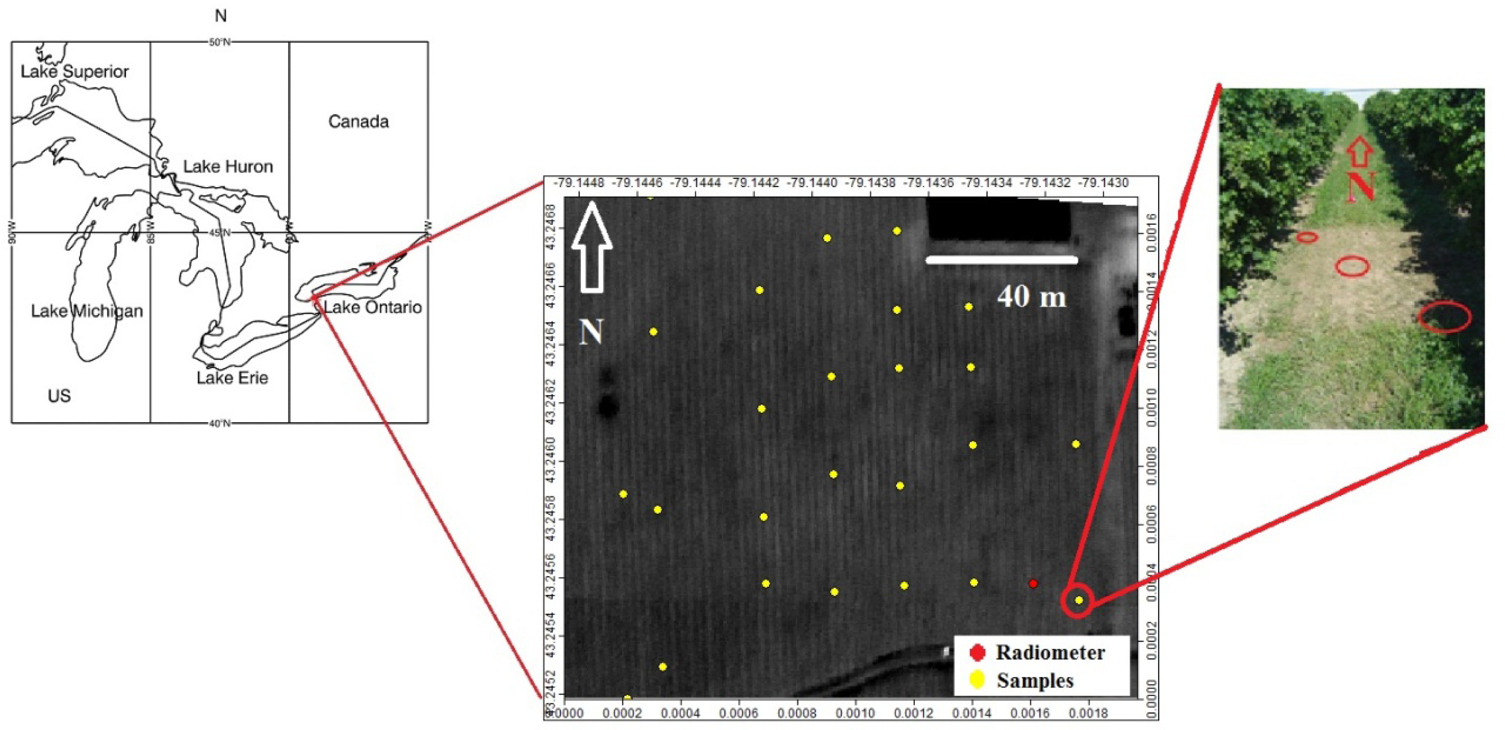
3.1. Study Area
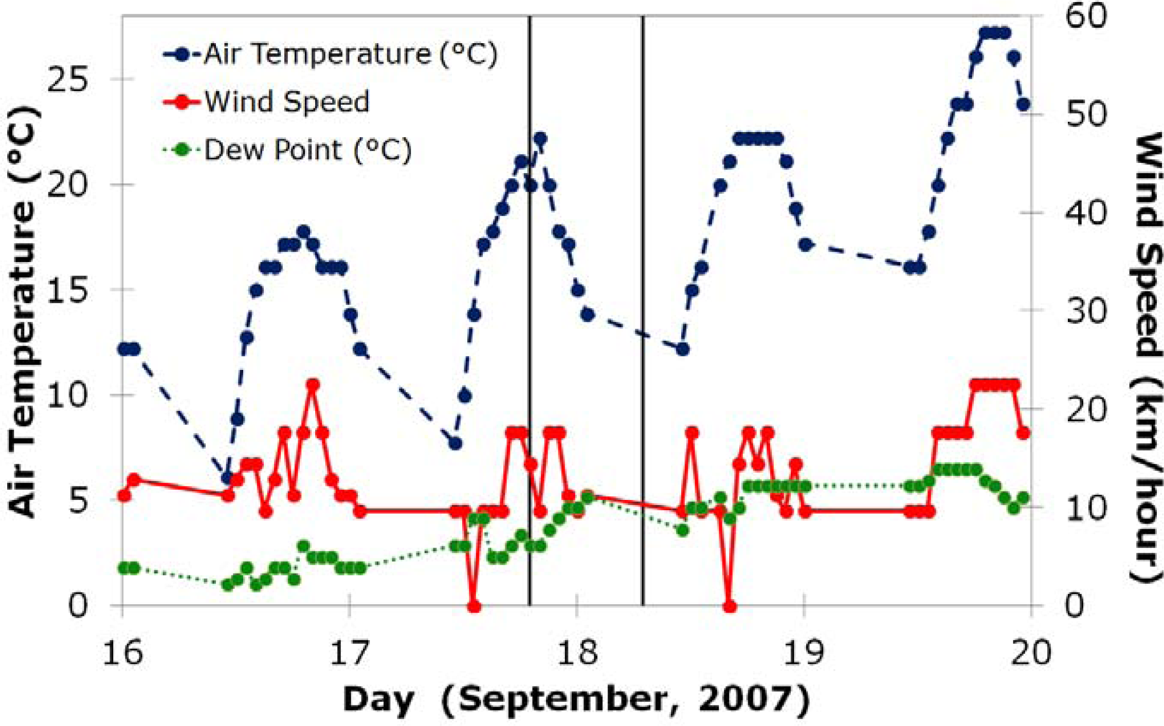
3.2. Fieldwork and Data Collection
3.3. Aerial Mapping of Thermal Inertia
3.4. Calculating Thermal Inertia
3.5. Statistical Analysis
4. Results
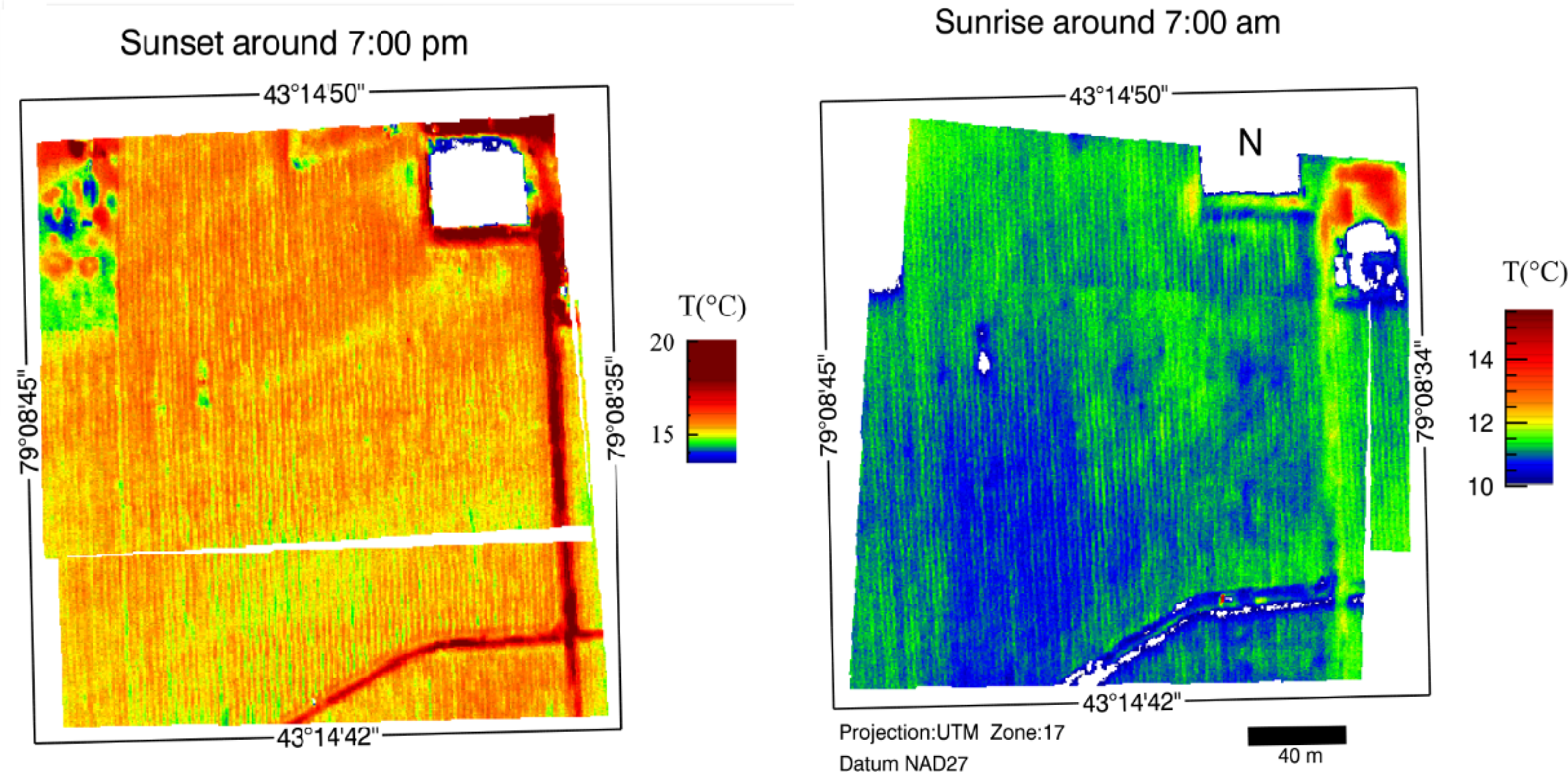
4.1. Aerial Thermal Imagery
4.2. Soil Physical Properties
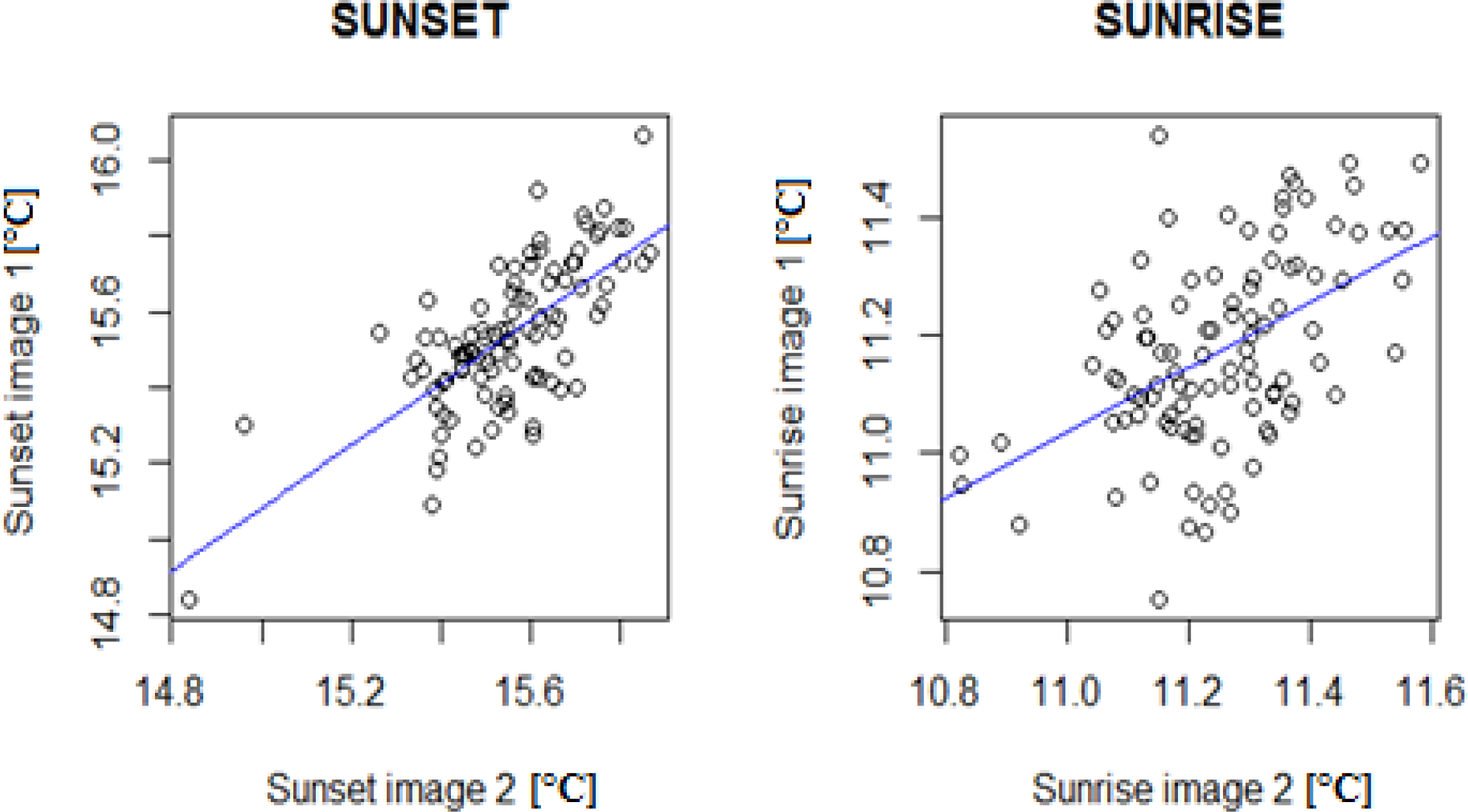
4.3. Relationships between Field Measurements and Remote Sensing Imagery
4.4. Regression Relationships between Thermal Inertia and Soil Properties
5. Discussion
5.1. Thermal Inertia and Soil Properties
5.2. Advantages of Remotely-Sensed Thermal Inertia
5.3. Limitations of Field Estimated Thermal Inertia
5.4. Improving Moisture Retrieval Using Thermal Inertia
6. Conclusions
Acknowledgments
Conflict of Interest
References and Notes
- Bramley, R.; Proffitt, A.P.B. Managing variability in viticultural production. Austr. Grapegrower Winemaker 1999, 427, 11–16. [Google Scholar]
- Lamb, D.W.; Bramley, R.G.V. Managing and monitoring spatial variability in vineyard productivity. Nat. Resource Manage 2001, 4, 25–30. [Google Scholar]
- Bramley, R. Generating Early Financial Benefits from Precision Viticulture through Selective Harvesting. Proceedings of the 5th European Conference on Precision Agriculture, Uppsala, Sweden, 9–12 June 2005.
- Bramley, R.G.V.; Proffitt, A.P.B. Variation in Grape Yield and Quality in a Coonawarra Vineyard. Proceedings of the 5th International Symposium on Cool Climate Viticulture & Oenology, Melbourne, VIC, Australia, 16–20 January 2000.
- Lamb, D.W. The use of qualitative airborne multispectral imaging for managing agricultural crops—A case study in south-eastern Australia. Aust. J. Exp. Agr 2000, 40, 725–738. [Google Scholar]
- Lamb, D.W.; Bramley, R.G.V.; Hall, A. Precision viticulture—An Australian perspective. In Viticulture living with limitations. Acta. Hort 2002, 640, 15–25. [Google Scholar]
- Hall, A.; Lamb, D.W.; Holzapfel, B.; Louis, J. Optical remote sensing applications in viticulture—A review. Aust. J. Grape Wine Res 2002, 8, 36–47. [Google Scholar]
- Kaleita, A.L.; Tian, L.F.; Hirschi, M.C. Relationship between soil moisture content and soil surface reflectance. Trans. ASAE 2005, 48, 1979–1986. [Google Scholar]
- Bramley, R.G.V. Progress in the Development of Precision Viticulture—Variation in Yield, Quality and Soil Properties in Contrasting Australian Vineyards. In Precision Tools for Improving Land Management; Currie, L.D., Loganathan, P., Eds.; Massey University: Palmerston North, New Zealand, 2001; pp. 25–43. [Google Scholar]
- Lamb, D.; Mitchell, A.; Hyde, G. Vineyard trellising with steel posts distorts data from EM soil surveys. Aust. J. Grape Wine Res 2005, 11, 24–32. [Google Scholar]
- Bennett, W.B.; Wang, J.; Bras, R.L. Estimation of global ground heat flux. J. Hydrometeorol 2008, 9, 744–759. [Google Scholar]
- Tian, J.; Su, H.; Chen, S.; Zhang, R.; Yang, Y.; Rong, Y. Estimation of Soil Heat Flux by Apparent Thermal Inertia. Proceedings of 2011 IEEE International Geoscience and Remote Sensing Symposium, Vancouver, BC, Canada, 24–29 July 2011.
- Wang, J.; Bras, R.L. A model of evapotranspiration based on the theory of maximum entropy production. Water Resour. Res 2011, 47, 1–10. [Google Scholar]
- Wang, J.; Bras, R.L. Ground heat flux estimated from surface soil temperature. J. Hydrol 1999, 216, 214–226. [Google Scholar]
- Wang, J.; Bras, R.L.; Sivandran, G.; Knox, R.G. A simple method for the estimation of thermal inertia. Geophys. Res. Lett 2010, 37, 1–5. [Google Scholar]
- Price, J.C. Thermal inertia mapping: A new view of the Earth. J. Geophys. Res 1977, 82, 2582–2590. [Google Scholar]
- Verhoef, A. Remote estimation of thermal inertia and soil heat flux for bare soil. Agric. For. Meteorol 2004, 123, 221–236. [Google Scholar]
- Verstraeten, W.W.; Veroustraete, F.; Van der Sande, C.J.; Grootaers, I.; Feyen, J. Soil moisture retrieval using thermal inertia, determined with visible and thermal spaceborne data, validated for European forests. Remote Sens. Environ 2006, 101, 299–314. [Google Scholar]
- Pratt, D.A.; Ellyett, C. D. The thermal inertia approach to mapping of soil moisture and geology. Remote Sens. Environ 1979, 8, 151–168. [Google Scholar]
- Minacapilli, M.; Iovino, M.; Blanda, F. High resolution remote estimation of soil surface water content by a thermal inertia approach. J. Hydrol 2009, 379, 229–238. [Google Scholar]
- Minacapilli, M.; Cammalleri, C.; Ciraolo, G.; D’Asaro, F.; Iovino, M.; Maltese, A. Thermal inertia modeling for soil surface water content estimation: A laboratory experiment. Soil Sci. Soc. Am. J 2012, 76, 92–100. [Google Scholar]
- Price, J.C. On the analysis of thermal infrared imagery: The limited utility of apparent thermal inertia. Remote Sens. Environ 1985, 18, 59–73. [Google Scholar]
- Maltese, A.; Capodici, F.; Ciraolo, G.; La Loggia, G. Mapping soil water content under sparse vegetation and changeable sky conditions: Comparison of two thermal inertia approaches. J. Appl. Remote Sens 2013, 7, 73548. [Google Scholar]
- Maltese, A.; Bates, P.D.; Capodici, F.; Cannarozzo, M.; Ciraolo, G.; La Loggia, G. Critical analysis of thermal inertia approaches for surface soil water content retrieval. Hydrol. Sci. J 2013, 58, 1–18. [Google Scholar]
- Murray, T.; Verhoef, A. Moving towards a more mechanistic approach in the determination of soil heat flux from remote measurements—A universal approach to calculate thermal inertia. Agric. For. Meteorol 2007, 147, 80–87. [Google Scholar]
- Murray, T.; Verhoef, A. Moving towards a more mechanistic approach in the determination of soil heat flux from remote measurements II. Diurnal shape of soil heat flu. Agric. For. Meteorol 2007, 147, 80–87. [Google Scholar]
- Van Wijk, W.R. General Temperature Variations in a Homogeneous Soil. In Physics of Plant Environment, 1st ed; North-Holland Publishing Co.: Amsterdam, The Netherlands, 1963; pp. 144–169. [Google Scholar]
- Brunt, D. Notes on radiation in the atmosphere. I. Quart. J. R. Meteorol. Soc 1932, 58, 389–420. [Google Scholar]
- Xue, Y.; Cracknell, A.P. Advanced thermal inertia modelling. Int. J. Remote Sens 1995, 16, 431–446. [Google Scholar]
- Pratt, D.A.; Foster, S.J.; Ellyett, C.D. A calibration procedure for fourier series thermal inertia models. Photogramm. Eng. Remote Sensing 1980, 46, 529–538. [Google Scholar]
- Johansen, O. Thermal Conductivity of Soils. University of Trondheim, Trondheim, Norway, 1975; p. 213. [Google Scholar]
- Mo, T.; Choudhury, B.J.; Schmugge, T.J.; Wang, J.R.; Jackson, T.J. A model for microwave emission from vegetation-covered fields. J. Geophys. Res 1982, 87, 11229–11237. [Google Scholar]
- Oke, T.R. Leaves. In Boundary Layer Climates; Routledge: London, UK, 1988; Chapter 4.2; pp. 117–122. [Google Scholar]
- Kim, E.J.; England, A.W. Radiobrightness Thermal Inertia Sensing of Soil and Canopy Moistures for Grassland Areas. Proceedings of Second Topical Symposium on Combined Optical-Microwave Earth and Atmosphere Sensing, Atlanta, GA, USA, 3–6 April 1995; pp. 39–41.
- Wicklund, R.E.; Matthews, B.C. Soil Survey of Lincoln County, Ontario; Report Number 34; Canada Department of Agriculture. Research Branch: Guelph, ON, Canada, 1963; pp. 23–37. [Google Scholar]
- Reedy, R.C.; Scanlon, B.R. Soil water content monitoring using electromagnetic induction. J. Geotech. Geoenviron. Eng 2003, 129, 1028–1039. [Google Scholar]
- Soliman, A.; Brown, R.; Heck, R.J. Separating near surface thermal inertia signals from a thermal time series by standardized principal component analysis. Int. J. Appl. Earth Obs. Geoinf 2011, 13, 607–615. [Google Scholar]
- Pradel, E.; Pieri, P. Influence of a grass layer on vineyard soil temperature. Aust. J. Grape Wine Res 1993, 6, 59–67. [Google Scholar]
- Mira, M.; Valor, E.; Caselles, V.; Rubio, E.; Coll, C.; Galve, J.M.; Niclòs, R.; Sánchez, J.M.; Boluda, R. Soil moisture effect on thermal infrared (8–13 μm) emissivity. IEEE J. Sel. Top. Appl. Earth Obs 2010, 48, 2251–2260. [Google Scholar]
- Flir Systems Inc. User’s Manual Flir Tools/Tools+ 3.1; Flir Systems Inc.: Wilsonville, OR, USA, 2013; pp. 54–60. [Google Scholar]
- Endres, T. Personal Communication. 2012. [Google Scholar]
- Zweig, M.H.; Campbell, G. Receiver operating characteristic (ROC) plots: A fundamental evaluation tool in clinical medicine. Clin. Med 1993, 39, 561–577. [Google Scholar]
- Royall, R. M. The effect of sample size on the meaning of significance tests. Am. Stat 1986, 40, 313–315. [Google Scholar]
- Pinheiro, J.; Bates, D. Mixed-Effects Models in S and S-PLUS, 1st ed; Springer: New York, NY, USA, 2000; pp. 133–199. [Google Scholar]
- The R Project for Statistical Computing. Available online: http://www.R-project.org/ (accessed on 20 March 2013).
- Pinheiro, J.; Bates, D.; DebRoy, S.; Sarkar, D.; Team, T.R.C. nlme: Linear and Nonlinear Mixed Effects Models, 1st ed; R Foundation for Statistical Computing: Vienna, Austria, 2009; R package; pp. 186–195. [Google Scholar]
- Johnson, L.F.; Trout, T.J. Satellite NDVI assisted monitoring of vegetable crop evapotranspiration in California’s San Joaquin valley. Remote Sens 2012, 4, 439–455. [Google Scholar]
- Reitberger, J.; Schnörr, C.; Heurich, M.; Krzystek, P.; Stilla, U. Towards 3D mapping of forests: A comparative study with first/last pulse and full waveform LIDAR data. Int. Arch. Photogramm. Remote Sens. Spat. Inf. Sci 2008, 37, 1397–1404. [Google Scholar]
- Mathews, A.; Jensen, J. Visualizing and quantifying vineyard canopy LAI using an unmanned aerial vehicle (UAV) collected high density structure from motion point cloud. Remote Sens 2013, 5, 2164–2183. [Google Scholar]


| Measurement | Replicates | Proxy for |
|---|---|---|
| Bulk electrical conductivity (by EM38) | Horizontal mode perpendicular to vine rows Horizontal mode parallel to vine rows Vertical mode perpendicular to vine rows Vertical mode parallel to vine rows | Clay mineralogy and soil solution salinity given dry conditions |
| Mechanical resistance (by soil penetrometer) | Right slice of the vine row Middle of vine row Left slice of the vine row | Soil bulk density, soil compaction and stoniness |
| Soil dielectric constant (by Theta Probe) | Same as mechanical resistance sampling | Soil volumetric moisture content |
| TIR emissions (by thermal infrared gun) | Same as mechanical resistance sampling | Surface temperature |
| Flight Time | Estimated Surface Emissivity | Sky Temperature [°C] | Relative Humidity [%] | Air Temperature [°C] | Flight Height [m AGL] |
|---|---|---|---|---|---|
| 6:50 p.m.–7:03 p.m. 17 September 2007 | 0.94 | −1.4 | 40.5 | 20.6 | ≈ 490 |
| 7:11 a.m.–7:33 a.m. September 18, 2007 | 0.94 | −3.4 | 78.8 | 13.1 | ≈ 490 |
| Variable | Minimum | Lower Quartile | Median | Mean | Upper Quartile | Maximum |
|---|---|---|---|---|---|---|
| Apparent Electrical Conductivity Horizontal-Parallel Mode [mS/m] | 18.6 | 30.7 | 37.2 | 40.7 | 47.8 | 68.6 |
| Volumetric soil moisture (Theta Probe) [%] | 9.7 | 12.7 | 15 | 14.5 | 16.3 | 19.4 |
| Mechanical Resistance (average) [kPa] | 1,480 | 2,056 | 2,368 | 2,399 | 2,655 | 3,306 |
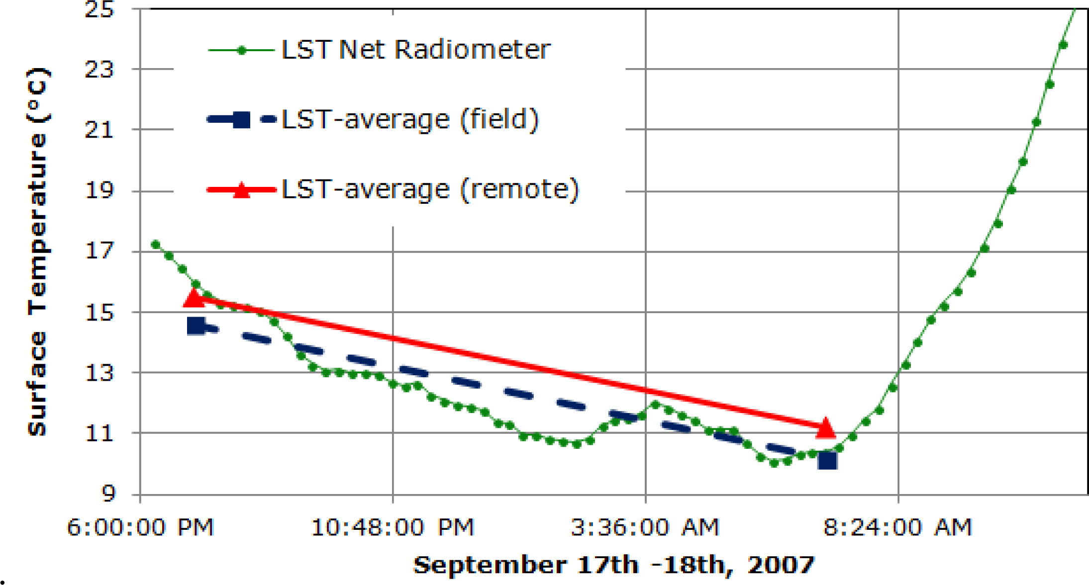
| LST-sunset (field) [°C] | 14.2 | 14.5 | 14.6 | 14.6 | 14.8 | 15 |
| LST-sunrise (field) [°C] | 9.6 | 10.1 | 10.2 | 10.2 | 10.4 | 10.7 |
| Lst-sunset (remote) [°C] | 15.2 | 15.5 | 15.5 | 15.5 | 15.6 | 15.9 |
| Lst-sunrise (remote) [°C] | 10.9 | 11.1 | 11.2 | 11.2 | 11.3 | 11.5 |
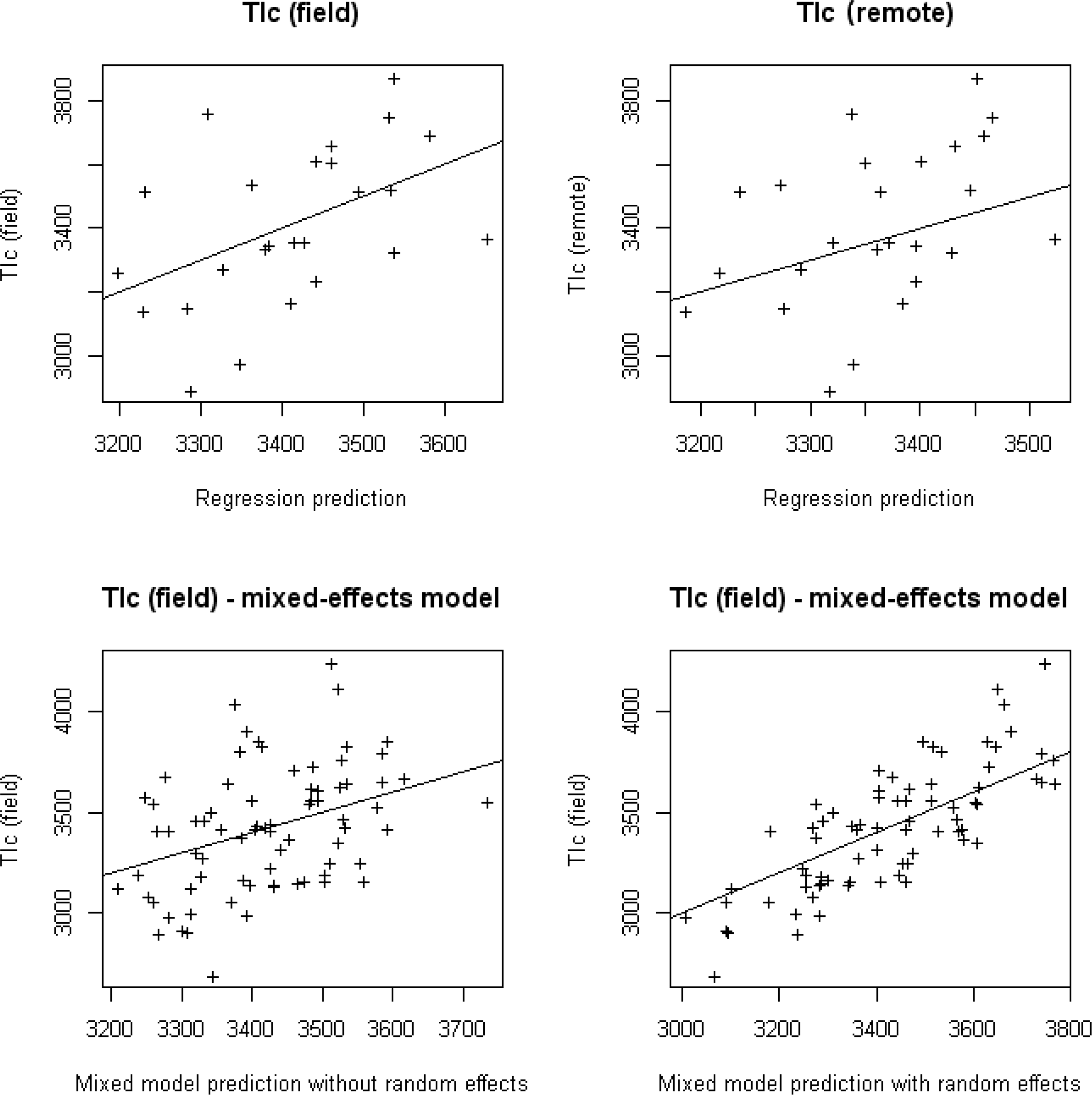
| TIc (field) [J·m−2·K−1·s−1/2] | 2,894 | 2,894 | 3,357 | 3,410 | 3,609 | 3,872 |
| TIc (remote) [J·m−2·K−1·s−1/2] | 3,068 | 3,287 | 3,348 | 3,361 | 3,430 | 3,581 |
| Variables | Correlation Coefficient (p-value) |
|---|---|
| LST (remote), LST (field) at local sunrise | 0.075 (p = 0.721) |
| LST (remote) vs. LST (field) at local sunset | 0.392 (p = 0.053) |
| TIc (remote) vs. TIc (field) | 0.374 (p = 0.065) |
| EM38 Horizontal Parallel | Theta Probe | Mechanical Resistance Average | Mechanical Resistance (0/1) | |
|---|---|---|---|---|
| TIc (field) | −0.057 | 0.392 | 0.108 | 0.699 |
| TIc (remote) | −0.351 | 0.500 | 0.167 | 0.706 |
| LST-sunset (field) | 0.199 | −0.274 | −0.326 | 0.688 |
| LST-sunrise (field) | 0.085 | 0.316 | −0.066 | 0.614 |
| Lst-sunset (remote) | 0.128 | −0.331 | −0.195 | 0.772 |
| Lst-sunrise (remote) | −0.267 | 0.249 | −0.001 | 0.522 |
| Response Variable | Intercept | Theta Probe | EM38 | Mechanical Resistance (0/1) | R2 (adjusted R2) | Residual Standard Deviation |
|---|---|---|---|---|---|---|
| TIc (field) | 2,863.72 | 34.57 | - | 138.17 | 0.224 | 227.2 |
| [17.59] | [97.73] | (0.153) | ||||
| (0.062) | (0.171) | |||||
| TIc (remote) | 3,118.101 | 21.365 | −2.313 | 81.965 | 0.416 | 105.6 |
| [8.265]* | [1.589] | [45.721] | (0.333) | |||
| (0.01)) | (0.160) | (0.087) | ||||
| TIc (field) In the mixed-effects model | 2,950.321 | 31.0470 | - | 139.143 | 0.167* | 287.9*** |
| [11.385] | [86.944] | 0.624** | ||||
| (0.009) | (0.116) |
© 2013 by the authors; licensee MDPI, Basel, Switzerland This article is an open access article distributed under the terms and conditions of the Creative Commons Attribution license ( http://creativecommons.org/licenses/by/3.0/).
Share and Cite
Soliman, A.; Heck, R.J.; Brenning, A.; Brown, R.; Miller, S. Remote Sensing of Soil Moisture in Vineyards Using Airborne and Ground-Based Thermal Inertia Data. Remote Sens. 2013, 5, 3729-3748. https://0-doi-org.brum.beds.ac.uk/10.3390/rs5083729
Soliman A, Heck RJ, Brenning A, Brown R, Miller S. Remote Sensing of Soil Moisture in Vineyards Using Airborne and Ground-Based Thermal Inertia Data. Remote Sensing. 2013; 5(8):3729-3748. https://0-doi-org.brum.beds.ac.uk/10.3390/rs5083729
Chicago/Turabian StyleSoliman, Aiman, Richard J. Heck, Alexander Brenning, Ralph Brown, and Stephen Miller. 2013. "Remote Sensing of Soil Moisture in Vineyards Using Airborne and Ground-Based Thermal Inertia Data" Remote Sensing 5, no. 8: 3729-3748. https://0-doi-org.brum.beds.ac.uk/10.3390/rs5083729