Article

NASA Goddard’s LiDAR, Hyperspectral and Thermal (G-LiHT) Airborne Imager

1
NASA Goddard Space Flight Center, Greenbelt, MD 20771, USA
2
Sigma Space Corporation, Lanham, MD 20706, USA
*
Author to whom correspondence should be addressed.
Remote Sens. 2013, 5(8), 4045-4066; https://0-doi-org.brum.beds.ac.uk/10.3390/rs5084045
Submission received: 20 June 2013 / Revised: 6 August 2013 / Accepted: 8 August 2013 / Published: 13 August 2013

Abstract

:
The combination of LiDAR and optical remotely sensed data provides unique information about ecosystem structure and function. Here, we describe the development, validation and application of a new airborne system that integrates commercial off the shelf LiDAR hyperspectral and thermal components in a compact, lightweight and portable system. Goddard’s LiDAR, Hyperspectral and Thermal (G-LiHT) airborne imager is a unique system that permits simultaneous measurements of vegetation structure, foliar spectra and surface temperatures at very high spatial resolution (∼1 m) on a wide range of airborne platforms. The complementary nature of LiDAR, optical and thermal data provide an analytical framework for the development of new algorithms to map plant species composition, plant functional types, biodiversity, biomass and carbon stocks, and plant growth. In addition, G-LiHT data enhance our ability to validate data from existing satellite missions and support NASA Earth Science research. G-LiHT’s data processing and distribution system is designed to give scientists open access to both low- and high-level data products ( http://gliht.gsfc.nasa.gov), which will stimulate the community development of synergistic data fusion algorithms. G-LiHT has been used to collect more than 6,500 km2 of data for NASA-sponsored studies across a broad range of ecoregions in the USA and Mexico. In this paper, we document G-LiHT design considerations, physical specifications, instrument performance and calibration and acquisition parameters. In addition, we describe the data processing system and higher-level data products that are freely distributed under NASA’s Data and Information policy.

Graphical Abstract

1. Introduction

LiDAR, hyperspectral and thermal remote sensing are core areas of current and planned NASA remote sensing capability (e.g., Landsat Enhanced Thematic Mapper Plus, ETM+, and Operational Land Imager, OLI; Earth Observing-1, Hyperion; Earth Observing System’s Advanced Spaceborne Thermal Emission and Reflection Radiometer, ASTER, Multi-angle Imaging SpectroRadiometer, MISR, and Moderate Resolution Imaging Spectroradiometer, MODIS; Suomi National Polar-orbiting Partnership Visible Infrared Imaging Radiometer Suite, NPP VIIRS; Ice, Cloud, and Land Elevation Satellite-2 Advanced Topographic Laser Altimeter System, ICESat-2; and Hyperspectral Infrared Imager, HyspIRI), and fusion of complementary data from different sensors offers the potential for improved global remote sensing of terrestrial ecosystems. Formation flying missions, such as NASA’s A-Train satellite constellation, offer near-simultaneous coverage from a number of Earth-observing systems; however, the spatial resolution of the current generation of NASA sensors limits some terrestrial ecology applications. Furthermore, efforts to merge 3D structure information from LiDAR with imaging spectrometer and thermal data is currently hindered by the absence of a LiDAR designed for vegetation in space [1] and an EO-1 satellite that is approaching the end of its useful life.
Airborne platforms are more flexible than satellite missions for developing and testing data fusion at fine spatial (1 to 10 m) and spectral resolutions, which have prompted a new generation of LiDAR and imaging spectrometer instrument packages [24]. Airborne platforms offer specific advantages for the study of terrestrial ecosystem, including targeted acquisitions of seasonal and diurnal processes (e.g., wetland inundation, plant phenology, drought and fire impacts) and coordinated field and remote sensing data collection needed to scale process-level understanding to the scale of airborne and satellite remote sensing observations [5]. Furthermore, the addition of coincident thermal data to LiDAR and imaging spectrometer data broadens the range of potential terrestrial ecology applications to include research on evapotranspiration, hydrology, forest health and urban applications [6,7].
Here, we describe the development of a unique multi-sensor instrument, Goddard’s LiDAR, Hyperspectral and Thermal (G-LiHT) airborne imager, which advances previous concepts for data fusion by integrating LiDAR, hyperspectral and thermal sensors in a lightweight and portable system for worldwide research applications. G-LiHT’s single-solution GPS-INS (Global Positioning System and Inertial Navigation System) avoids multi-dimensional data effects that are introduced when data is collected at different time and observational scales [2]. Imaging spectroscopy provides quantitative information on vegetation cover, species composition and biophysical and chemical properties that can be derived from measurements of reflected sunlight in the visible through shortwave infrared wavelengths [812]. Light detection and ranging provides quantitative, 3D information on terrain and vegetation cover, height and distribution of canopy elements, which can be used to characterize biodiversity and habitat [13] and estimate light interception in plant photosynthesis and production models [14]. Land surface temperature provides data needed to estimate evapotranspiration and other surface energy fluxes [6], and can be an indicator of soil or vegetation moisture status [15]. By using commercial off-the-shelf instrumentation and general aviation aircraft, G-LiHT also reduces development and operational costs. Low-cost deployment of the G-LiHT system opens a wide range of applications for targeted, airborne remote sensing, including diurnal and seasonal processes in terrestrial ecosystems at ∼1 m spatial resolution (Figure 1).
The goal of this multi-sensor and data fusion effort is to characterize ecosystem form and function using remote sensing data, with a particular emphasis on the data products needed to develop a new generation of high resolution ecosystem and radiative transfer models. Analysis of G-LiHT data will be used to:
  • provide new insight into photosynthetic functionality and vegetation productivity, including new, spatially-explicit remote sensing indicators of key dynamic biological processes;
  • characterize fine-scale spatial and temporal heterogeneity in ecosystem structure and function under diverse environmental and climate conditions; and
  • create new methods for data fusion to monitor ecosystem health and the effects of climate and human-induced changes on these ecosystems.

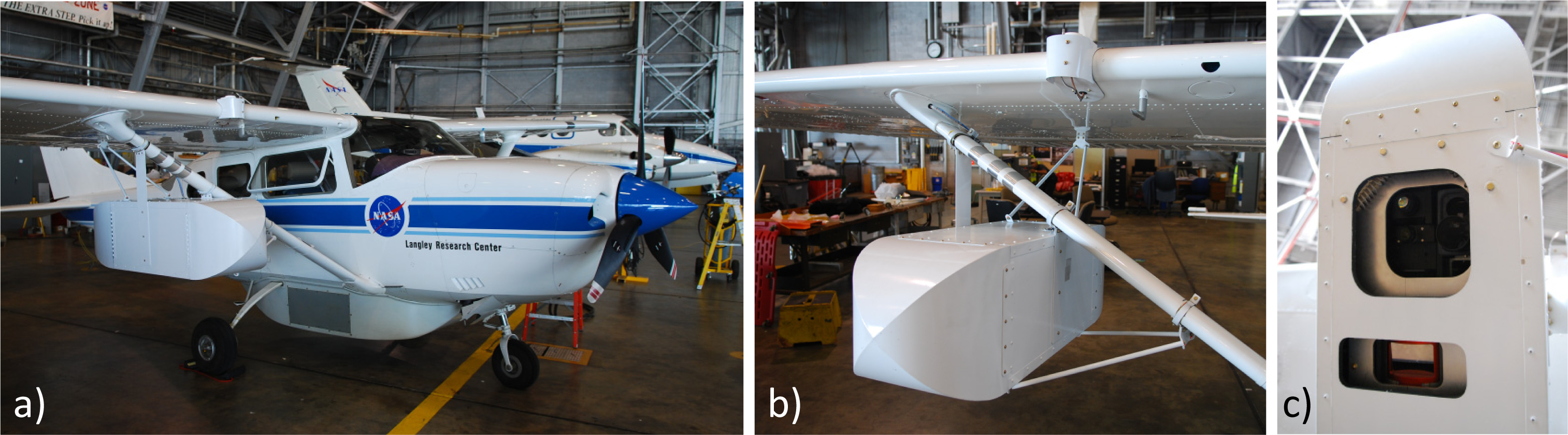
2. G-LiHT Design and Instrumentation

2.1. Scientific Objectives and Design Considerations

G-LiHT was designed as a relatively inexpensive, robust and portable research tool for evaluating the potential benefits of data fusion for studies of terrestrial ecosystems. Table 1 lists the objectives and related measurement requirements for G-LiHT. One of the major obstacles to the development of science-based data fusion algorithms is the availability of accurately co-registered data of similar grain size for different information types. This is often the case when instruments are flown on different platforms and acquired on different dates. We believe that “instrument fusion” is a prerequisite to “data fusion” and conceived G-LiHT as a multi-sensor airborne imaging system that would simultaneously map the composition, structure and function of terrestrial ecosystems.
In addition, G-LiHT was designed to simplify worldwide deployment and minimize collection and data processing costs. As a result, G-LiHT features eye-safe lasers, a portable, low-power payload (37 kg; 30 × 30 × 60 cm; 210 W), a single-solution GPS-INS, compatibility with common, civilian-use aircraft (e.g., Cessna, Piper, Twin Otter; 12/28 VDC compatibility) using a standard camera port or custom wing-mounted pod and commercial off-the-shelf (COTS) instruments that are easy to replace and not regulated by ITAR (International Traffic in Arms Regulation). Both G-LiHT science and deployment objectives are traced to instrument and design requirements in Table 1.
G-LiHT instruments were physically arranged to fit in a rigid, compact package (Figure 2), with the scanning LiDAR, imaging spectrometer, hyperspectral and thermal camera aligned along an optical axis parallel to the flight path. Wire rope isolators (WR4-200-10, Endine Inc., Orchard Park, NY, USA) are used to mount the instrument package to the aircraft and reduce the impact of high-frequency aircraft vibrations. The system is weather resistant and can be mounted either internally to the aircraft over an appropriately sized view port or externally attached to aircraft using a custom fabricated pod. A custom pod was designed and fabricated by NASA for any Cessna 206, using mounting points that are standard on this platform (Figure 3).
Specifications of the individual G-LiHT instruments are provided in the sections below.

2.2. GPS and Inertial Navigation System (INS)

A single-solution GPS-INS (RT-4041, Oxford Technical Solutions, Oxfordshire, UK) is used to obtain high precision position and attitude measurements for all G-LiHT sensors. The unit is directly attached to the airborne laser scanning (ALS), which shares the same mounting plate as the optical breadboard for the imaging spectrometer and thermal camera (Figure 2). The GPS-INS incorporates a six-axis inertial navigation system (three gyroscopes and three servo-grade accelerometers) and an L1/L2 GPS (Global Positioning System) and GLONASS (Global Navigation Satellite System) receiver with an OmniStar decoder to deliver 10 cm positioning, 0.1° heading and 0.03° roll and pitch accuracies. Measurements are acquired at 250 Hz, which is required to geolocate data from the optical imagers (25 to 50 Hz) and ALS (300 kHz laser). The real-time internal processing includes strap down algorithms, a WGS-84 and EGM96 (Earth Gravitational Model 1996) Earth model, Kalman filtering and in-flight alignment algorithms. The Kalman filter and in-flight algorithms monitor the performance of the system and update the measurements to correct for inertial sensor errors and maintain high positional accuracy.

2.3. Airborne Scanning LiDAR

The VQ-480 (Riegl USA, Orlando, FL, USA) airborne laser scanning (ALS) instrument was selected for use with G-LiHT, because it was affordable, compact, provided evenly distributed pulses on the ground and offered near-turnkey operation. The VQ-480 uses a high-performance laser rangefinder and a rotating polygon mirror with three facets to deflect a 1,550 nm Class 1 laser beam onto the ground. A user-selectable pulse repetition rate up to 300 kHz provides an effective measurement rate of up to 150 kHz along a 60° swath perpendicular to the flight direction (Figure 3). A laser beam divergence of 0.3 mrad produces a 10 cm diameter footprint at the nominal operating altitude of 335 m. The small footprint laser beam allows detection of small gaps in the canopy and the ability to characterize fine scale disturbances, which are difficult to deconvolve from large footprint LiDAR waveforms (Figure 4, [17]). The mirror speed is set to a maximum of 100 rotations s−1 during G-LiHT acquisitions, whose points are spaced 0.23 m apart within a line perpendicular to the flight direction and 0.57 m between lines with a nominal aircraft speed of 110 knots. For each laser shot, the return waveform is digitized, and online processing algorithms are used to provide ranging data for multiple targets. Up to eight discrete ranging returns may be identified and recorded for a given pulse. Each return target is time tagged and accurately synchronized with the GPS-INS using a 1 Hz Transistor-Transistor Logic (TTL) pulse. Riegl’s software, RiACQUIRE, provides a graphical user interface for scanner control and near real-time monitoring of scanning LiDAR and GPS-INS data.

2.4. Profiling LiDAR

G-LiHT’s profiling LiDAR is an LD321-A40 (Riegl USA, Orlando, FL, USA), multi-purpose laser distance meter that is similar to the LD90-3800-VHS used in the Portable Airborne Laser System (PALS) [16]. The LD321-A40 provides a continuous profile of canopy height measurements, which, from a regional sampling perspective, provides data similar to other space-based profilers that have been flown (Ice, Cloud, and Land Elevation Satellite Geoscience Laser Altimeter System, ICESat GLAS), proposed for flight (Deformation, Ecosystem Structure and Dynamics of Ice, DESDynI) or which may be flown in the near future (ICESat-2 ATLAS). In addition, profiling data is important for studying horizontal landscape patch structure [13] and ensuring continuity between ALS and PALS datasets that have been collected worldwide. Real-time digital echo signal processing with the LD321-A40 enables precise distance measurement for complex multi-target situations, resolving up to five target distances per pulse. Distance measurements parallel to the flight line are used to continuously measure vegetation height and structure along a sampling transect. A Class 1M laser diode emits a 905 nm beam with a divergence of 1.5 mrad to produce a 50 cm diameter footprint at the nominal operating altitude of 335 m.

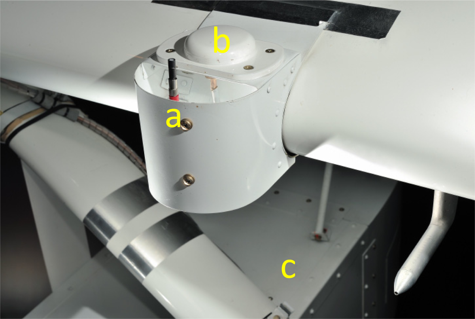
2.5. Irradiance Spectrometer

Downwelling irradiance is measured with an Ocean Optics (Dunedin, FL, USA) USB4000-VIS-NIR spectrometer. Light energy is transmitted to the spectrometer through an upward looking opaline glass cosine diffuser with a 180° field of view (FOV). The cosine diffuser is mounted on top of the aircraft, where there is an unobstructed view of the sky. A custom mount was designed for the leading edge of the Cessna 206 (Figure 5), which integrates both the GPS antenna and cosine diffuser. A 3 m long, 100 μm diameter optical fiber delivers the light energy through a 25 μm entrance slit and a multi-bandpass order-sorting filter, where it is dispersed with a fixed grating across a 3,648-element Toshiba linear Charge Coupled Device (CCD) array. The spectrometer covers the spectral range from 350 to 1,100 nm with a native optical resolution to ∼1.5 nm (full width half maximum, FWHM). Power and communications are transferred through a USB 2.0 connection to the computer. The downwelling radiometer is operated continuously during flight with a 33 ms integration time, a 30 scan average and 3× spectral binning, which is equivalent to a 1 Hz data acquisition rate. The unit is cross-calibrated with the imaging spectrometer to enable atmospheric characterization of downwelling irradiance, which is used to compute the at-sensor reflectance product.

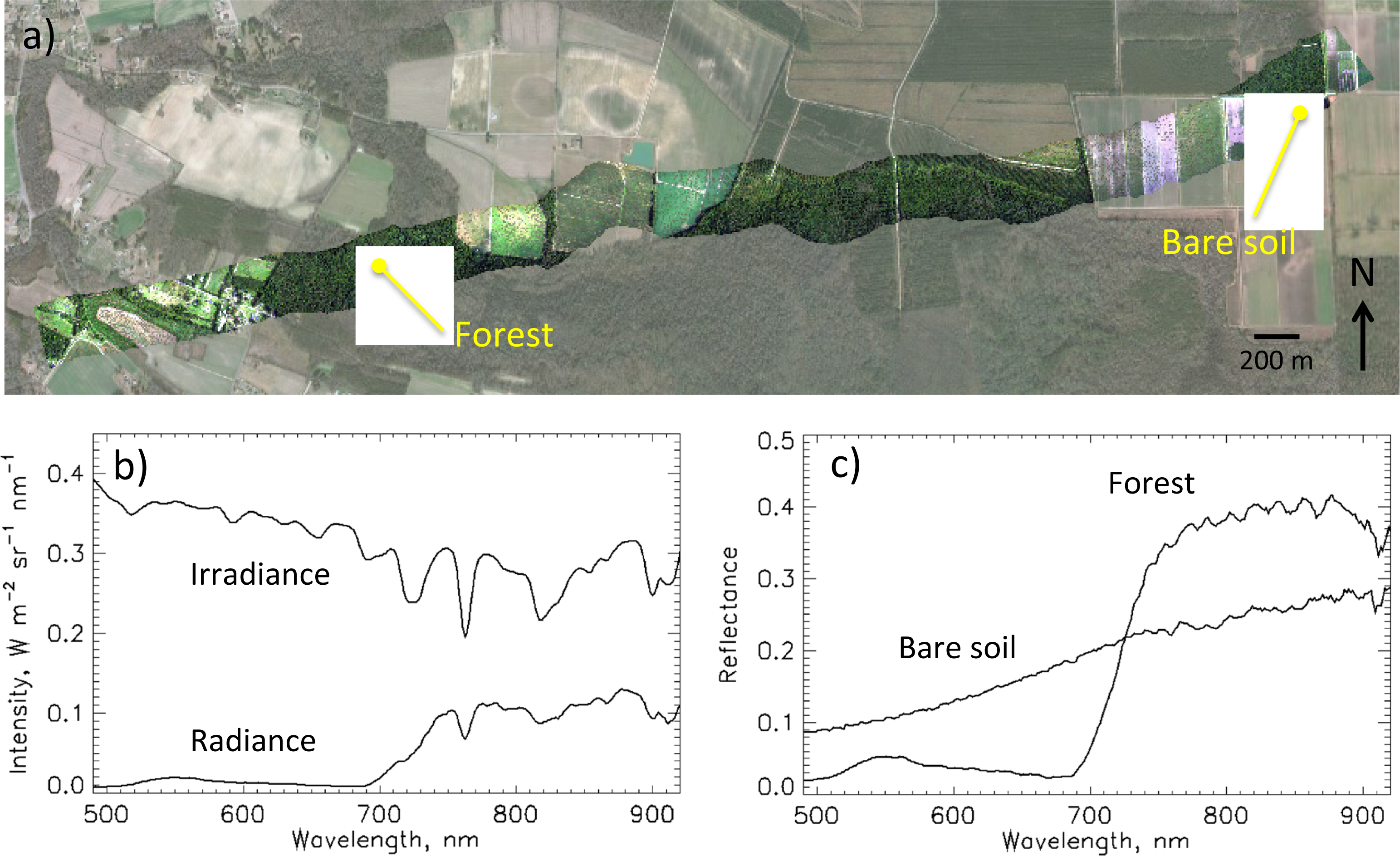
2.6. Imaging Spectrometer

The Hyperspec imaging spectrometer (Headwall Photonics, Fitchburg, MA, USA) enables high spectral and spatial resolution imaging by using f/2.0 telecentric optics and a high efficiency aberration-corrected convex holographic diffraction grating, providing an optical dispersion of 100 nm per mm over a 7.4 mm spatial by 6.0 mm spectral focal plane. The imaging spectrometer is based on the Offner form and is designed to operate in the 400–1,000 nm spectral region with a 50° full field of view. The Hyperspec imaging spectrometer accepts a C-mount objective lens (Cinegon f/1.4 8 mm, Schneider Optics, Hauppauge, NY, USA) with high optical performance using ultralow dispersion glass and broadband anti-reflection coating designed for the visible to near-IR spectrum. Coupled to the spectrometer is the RA1000 m/D high speed rugged megapixel focal plane array that allows 50 progressive frames per second to be acquired through an EPIX (Buffalo Grove, IL, USA) PIXCI ECB1 PCI Express CameraLink interface. The camera uses a 1,004 × 1,004 pixel 2/3-inch format interline CCD with 7.4 μm square pixels and 12-bit radiometric resolution. Other camera features include a digital fine gain for adjustable camera sensitivity over a 60 dB dynamic range, electronic shuttering and low smear characteristics. The camera is controlled with the serial communication channel of the CameraLink interface. Each image frame is coded with a computer timestamp synchronized with a Time Tools (Dudley, UK) LC2750 GPS Timing Receiver for post-processing geolocation using data from the GPS-INS detailed in Section 2.2 (Figure 6).

2.7. Thermal Imaging

G-LiHT’s thermal remote sensing capability originates from the Gobi-384 thermal imaging camera (Xenics, Leuven, Belgium). The instrument measures long wave infrared (LWIR) radiation over a broad spectral range (8 to 14 μm) using an uncooled amorphous silica (ASi) microbolometer detector with 384 cross track pixels and a 30° FOV. This compact camera (72 × 60 × 50 mm) uses a Gigabit Ethernet TCP/IP (Transmission Control Protocol and the Internet Protocol) interface to deliver 16-bit radiometrically calibrated thermal imaging data at a 25 Hz frame rate to the computer running Xenics’s Xeneth infrared camera software. Each image frame is coded with a computer timestamp synchronized to a GPS Timing Receiver (see Section 2.6).

3. Calibration

3.1. Boresight Alignment

Georeferenced LiDAR returns and optical observations are computed as a function of lever arm offsets, boresight angles and optical measurements. Bias in any of these parameters and GPS-INS errors will result in offset point clouds and distorted images. Boresight biases are computed using data collected over buildings with peaked roofs, where overlapping data are collected with different headings. Boresight corrections are computed between campaigns and consistently result in an accuracy of ∼10 cm (1 σ).

3.2. Radiometric Calibration

The absolute spectral response (ASR) of G-LiHT’s imaging spectrometer was calculated using measurements made with a portable version of the US National Institute of Standards and Technology’s (NIST) Spectral Irradiance and Radiance Responsivity Calibrations Using Uniform Sources (SIRCUS) [18], which is currently housed at NASA Goddard Space Flight Center (GSFC). SIRCUS uses continuously tunable lasers coupled to an integrating sphere as a radiance source for the calibration of detectors operating in the solar reflective spectrum. SIRCUS and appropriately characterized transfer radiometers allow absolute radiometric calibration with uncertainties of 0.5% and traceability to national standards [19]. The availability of lasers determines the spectral coverage on SIRCUS, and the uncertainties achievable are determined by the quality of the transfer radiometers and measurement technique. The high power and wavelength stability of the laser-based sources enable large aperture instruments to be characterized and calibrated. All irradiance and radiance responsivity calibrations are traceable to NIST’s Primary Optical Watt Radiometer (POWR) through regularly characterized transfer radiometers. The short calibration chain from NIST’s Primary Optical Watt Radiometer (POWR) to the transfer radiometer and imaging spectrometer minimizes the uncertainty of the Spectral Radiometer Facility (SRF). Spectral radiance calibrations at power levels typical of solar irradiance values allowed for quantitative measurements of the spectral response functions and under flight-like conditions over the focal plane from 415 to 1,020 nm. In addition to providing spectral and radiometric calibration, the combination of full-field, full-aperture and near-monochromatic method of radiometric calibration used here allows the unique capability of assessing and correcting for the total system stray light of the imaging spectrometer, not possible with traditional broadband calibration sources.

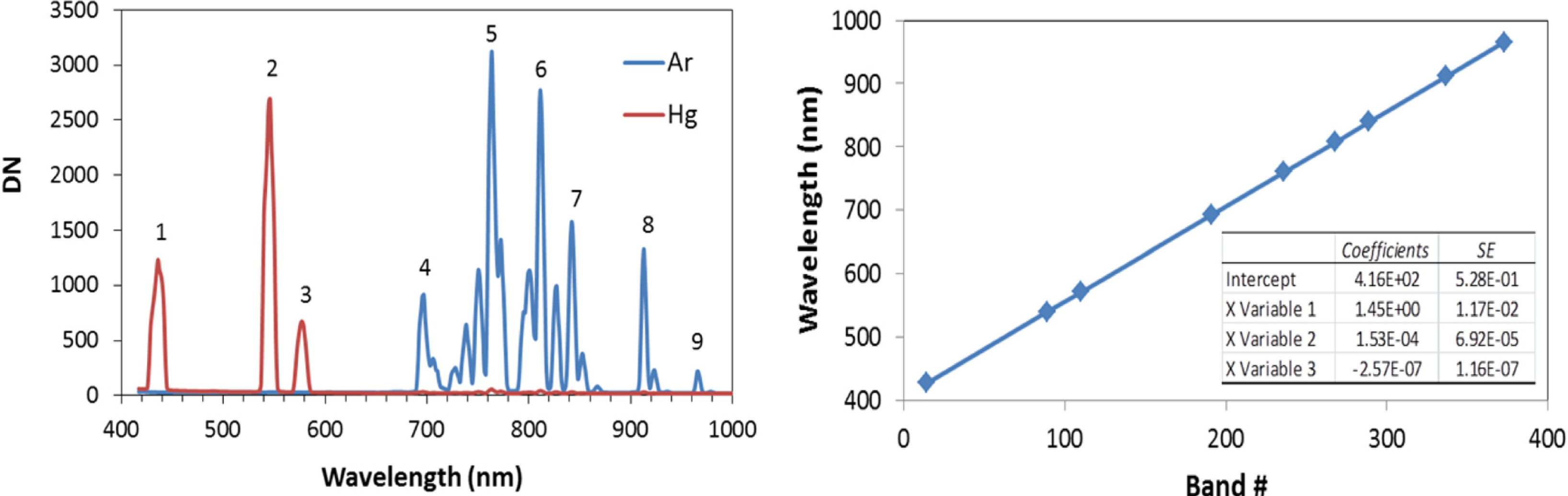
3.3. Wavelength and Radiometric Stability

Both the downwelling irradiance and upwelling imaging spectrometer are monitored for radiometric and wavelength stability. A portable, 10 cm Teflon integrating sphere with a Hg and Ar pen lamp illumination sources produce nine pronounced emission lines (Figure 7) that are used periodically to verify the spectral channel to wavelength relationship over the detector spectral range with sub-nanometer precision. A large aperture, 1 m integrating sphere and an NIST traceable uniform source is used to monitor the radiometric stability and performance of the spectrometers between campaigns.

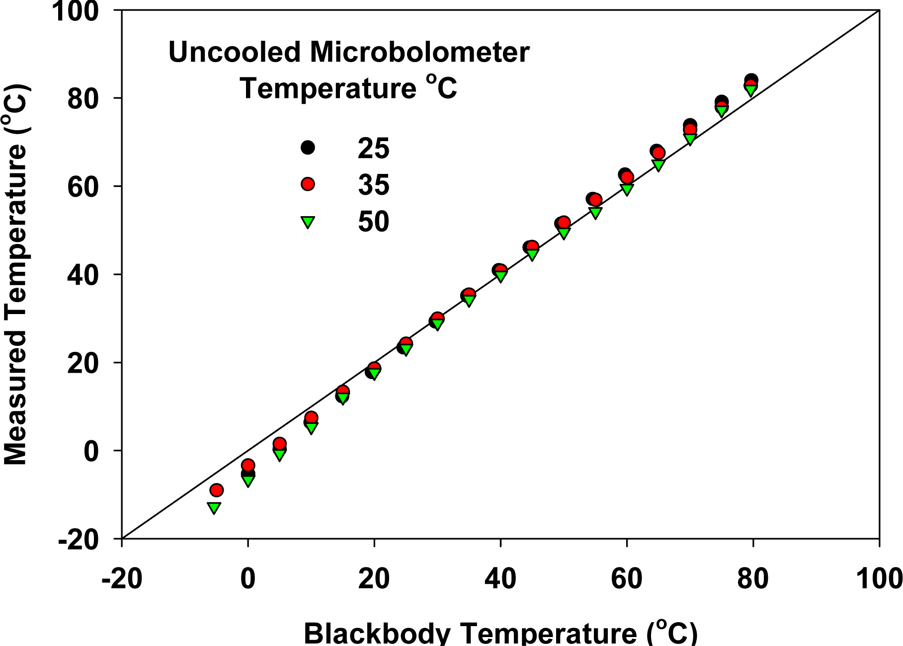
3.4. Thermal Radiometric Calibration

G-LiHT’s thermal imaging camera has factory radiometric calibration for surface temperatures between −20 °C and 120 °C, with a Noise Equivalent Temperature Difference (NETD) >50 mK. This wide dynamic range allows for airborne operations of the thermal image over a diverse range of surface temperatures. Thermal calibration stability as a function of a microbolometer operating temperature range of 25 °C to 50 °C was verified against a GSFC Calibration Facilities blackbody for stable operation over the target temperature range of −5 °C to 85 °C (Figure 8).

4. Flight Planning and Data Acquisition

Flight plans are made with X-TRACK Flight Management Software Suite (Track’Air Aerial Survey Systems, Oldenzaal, The Netherlands), using a nominal flight altitude of 335 m AGL, 60° FOV and 30% swath overlap. This configuration results in a LiDAR, spectrometer and thermal swath of 387, 310 and 173 m. The pixel size of the pushbroom imaging spectrometer is ∼1 m and is limited by the aircraft speed and frame acquisition rate. The instantaneous per pixel resolution of the thermal camera is approximately 3 times coarser than the imaging spectrometer, but oversampling with the 2D detector allows us to create a product of equal resolution (Section 5.2.4).
Flight lines are uploaded onto a 696 GPS (Garmin International, Inc., Olathe, KS, USA) for pilot navigation and onto the instrument operator’s computer, which is using Reigl’s RiAcquire acquisition software. Each instrument is separately controlled and triggered to collect data using vendor-supplied software. Ejectable, solid state hard drives provide fast input/output and quick retrieval upon conclusion of the flight.

5. Data Products, Processing and Distribution

5.1. Data Products

NASA’s Earth Science Data Systems program references data products based on their level of processing, ranging from Level 0 to Level 4 [20]. Level 0 (L0) data products include unprocessed instrument data; Level 1 (L1) products are time-referenced data that have been processed to at-sensor radiometric units; Level 2 (L2) products are geophysical variables derived from L1 products; and Level 3 (L3) products are geophysical variables mapped on a space-time grid scale. G-LiHT data products (L1 through L3) are listed in Table 2 for each of the instruments. Many of these products will help end users create additional higher-order products (e.g., solar and view angles are needed for computing bidirectional corrected reflectance; terrain and canopy heights are needed for orthorectification) and facilitate scientific data analysis (e.g., cloudiness and solar illumination conditions affect canopy photosynthesis) [21].

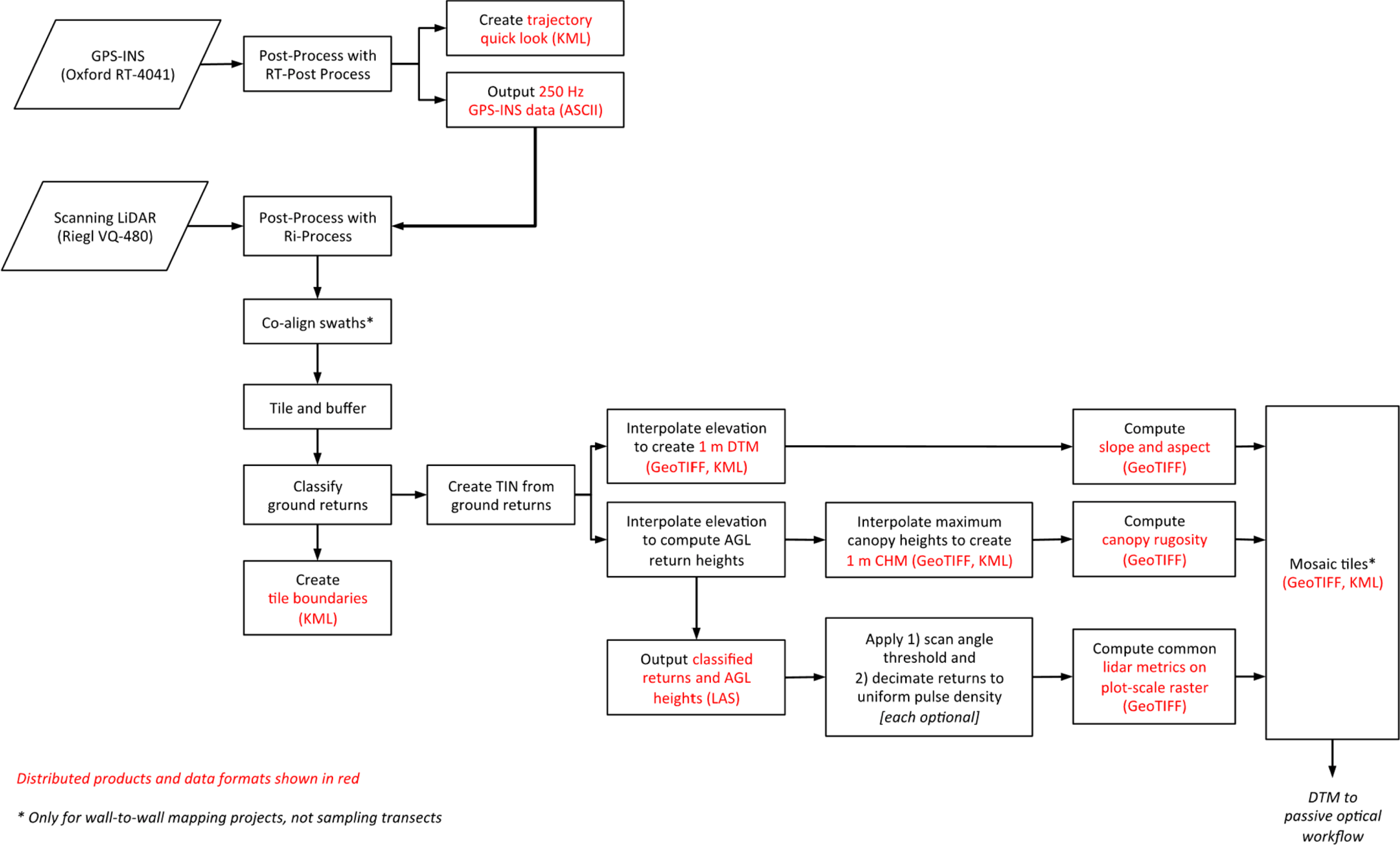
5.2. Data Processing System

An automated data processing system is key to releasing standardized products in a timely manner. Data processing begins with the GPS-INS and scanning LiDAR data, since some of the products are used in processing the imaging spectrometer and thermal data. Workflows for the scanning LiDAR and spectrometer data have been developed as illustrated in Figures 9 and 10. Manual pre-processing of L0 data with vendor supplied software is the first step in the workflows, followed by automated data processing algorithms that have been custom coded in the IDL-ENVI (Interactive Data Language and Environment for Visualizing Images) scientific programing language (Exelis Visual Information Solutions, Boulder, CO, USA). The following sections describe the specific data processing steps.

5.2.1. GPS and Inertial Data

GPS-INS data is stored on internal memory in a raw, unprocessed format. Lever arm and other offset coefficients are applied to the L0 data with Oxford’s RT Post Process software, which converts the proprietary binary data to an ASCII format. During this step, the inertial data is processed forwards and backwards in time to minimize the effects of GPS data drift. During data acquisition, OmniStar HP differential correction service provides a real-time positioning error of <15 cm in extended periods of open sky. Increased precision can be achieved where base station GPS data is available.

5.2.2. Scanning LiDAR Data

Riegl’s RiPROCESS software is used for managing, processing, analyzing and visualizing data acquired with the ALS system. RiPROCESS ingests raw laser scanner data and pre-processed GPS-INS data, applies calibration information, transforms the scan data into geographic coordinates and exports return data in LAS file format [22]. For mapping projects, individual swaths are co-aligned for small differences (typically <0.5 m) in elevation due to differences in position uncertainty, which is typically an effect of different satellite configurations and atmospheric conditions. A cross-track swath is typically collected at the conclusion of a mapping project to serve as a reference point for swath co-alignment.
LiDAR returns are resampled and processed as smaller data volumes (∼1 km tiles for mapping and ∼7 km segments for sampling transects) for efficient processing. Tiles are buffered to prevent edge artifacts during ground classification and creation of the Digital Terrain Model (DTM). Classification of ground returns is performed with a progressive morphological filter [23]. Delaunay triangulation is used to create a Triangulated Irregular Network (TIN) of ground hits, and the TIN is used to linearly interpolate DTM elevations on a 1 m raster grid. Additionally, the TIN is used to interpolate the base elevation of every non-ground return, and vegetation heights are computed by difference. A Canopy Height Model (CHM) is created by selecting the greatest return height in every 1 m grid cell, using these points to create a TIN and interpolating canopy heights on a 1 m raster grid. An example of the DTM and CHM models are shown in Figure 11. For mapped areas, tiles are mosaicked, and terrain slope and aspect, canopy rugosity (standard deviation of height) and common LiDAR metrics [24,25] are derived from the resulting data at the scale of a US Forest Service Forest Inventory and Analysis (FIA) field subplot (7.32 m radius).

5.2.3. Imaging Spectrometer Data

Pre-processing of the image spectrometer data requires the use of XCAP software (EPIX, Inc., Buffalo Grove, IL, USA) to convert L0 data in a proprietary VIF format to ASCII time stamps and an image cube in standard Band Interleaved by Line (BIL) format. Calibration coefficients (see below) are applied to both the downwelling irradiance data and upwelling imaging spectrometer data to compute at-sensor radiance (Figure 6). Prior to computing at-sensor reflectance, irradiance spectra are resampled spectrally to match the imaging spectrometer. Two reflectance products are computed as part of the workflow: at-sensor reflectance is computed as the fraction of irradiance detected by the imaging spectrometer, and surface reflectance is computed using the radiometric data and an atmospheric correction algorithm. Following the reflectance calculations, data are aggregated from the 1.5 nm native sampling interval using a Gaussian-based spectral resampling procedure to generate a distribution product with uniform 5 nm FWHM band spacing. This is a finer sampling and spectral resolution than is reported for NASA’s Next Generation Airborne Visible/Infrared Imaging Spectrometer (AVIRISng) [26] and may be useful for measuring fine spectral features, such as solar induced fluorescence [27]. From the reflectance data, common vegetation indices for greenness (e.g., Normalized Difference Vegetation Index, (NDVI); Enhanced Vegetation Index, (EVI); red edge), light use efficiency (e.g., Photochemical Reflectance Index) and leaf pigments (e.g., carotenoid, anthocyanin) are computed.
Each pixel in the image cube is georeferenced using Geo-Correction for Airborne Platforms (GCAP) [28], a software package developed at NASA Goddard Space Flight Center that provides the user the capability to georeference a raster image using the image time stamps and GPS-INS data. Pixel coordinates are used to build a geographic lookup table in ENVI that is distributed with the radiance data cube and is used to create georeferenced layers for the reflectance data, vegetation indices and ancillary data products.
Ancillary data products include valuable information for each pixel of the image cube, including: acquisition time, solar zenith angle, solar azimuth, incoming PAR, cloudiness index [21], aircraft elevation, aircraft altitude AGL, view angle and view azimuth. These time-space variables are computed from the LiDAR-derived DTM and a clear sky irradiance model [29]. The products will help end users create additional higher-order products (e.g., solar and view angles are needed for computing bidirectional corrected reflectance; terrain and canopy heights are needed for orthorectification) and facilitate scientific data analysis (e.g., cloudiness and solar illumination conditions affect canopy photosynthesis).
Future development will focus on improved co-registration through automated control points and implementing orthorectification and atmospheric correction algorithms specifically designed for low altitude, wide FOV airborne imagers [30].

5.2.4. Thermal Data

By selecting a single line of cross-track pixels from the thermal image array, the thermal data can be treated as a line imager in the same manner as the imaging spectrometer. However, the number of cross track pixels in a single line and frame rate limits the product to a coarse spatial resolution (∼3 m) using this method. Since the field of view of the full array is much greater than the spacing between images, we can use spatial oversampling techniques to create a smoothed, fine resolution (1 m) temperature product. We might also use additional information from the LiDAR and imaging spectrometer (e.g., land cover) to resolve non-linear edge effects, such as abrupt land cover boundaries [31]. Both of these methods for deriving fine-resolution surface temperature products are currently under development.

5.2.5. Profiling LiDAR Data

Level 0 profiling LiDAR data is captured in ASCII format through a 10/100 Mbit TCP/IP port, and can be processed in the same manner as PALS data [16].

5.3. G-LiHT Data Distribution

NASA’s Earth Science Program promotes the full and open sharing of data with all users in accordance with NASA’s Data and Information Policy [32], and this includes G-LiHT data products. Every effort is taken by the G-LiHT instrument team to ensure that accurate, well-calibrated data is released in a timely manner, and data is distributed in common, readily usable file formats. Classified LiDAR returns and feature heights are made available in ASPRS LAS file format (American Society for Photogrammetry and Remote Sensing, LASer file format), a non-proprietary, binary file industry standard [22]. This open data file format allows for the raw data and information specific to data collection to be recorded (e.g., scan angle, return number, classification, AGL height). Gridded LiDAR products are made available as GeoTIFF files that conform to established Tagged Image File Format (TIFF) interchange format for georeferenced raster imagery [33]. GeoTIFF files include geographic metadata formally, using compliant TIFF tags and structures. Multiband products from the imaging spectrometer will be distributed in standard Band Interleaved by Line (BIL) format. In addition to the data files, quick look images of key spatial variables (e.g., aircraft trajectory, DTM, CHM, true color image) created in Keyhole Markup Language (KML) [34] for visualization in Google Earth.
The data archive for G-LiHT products can be through the G-LiHT webpage, http://gliht.gsfc.nasa.gov or by directly connecting to the anonymous ftp site, fusionftp.gsfc.nasa.gov/ G-LiHT. The G-LiHT website contains additional instrument specifications, a description of various airborne campaigns, software tools and links to open source data analysis and visualization software. G-LiHT has been used to collect more than 6,500 km2 of data for NASA-sponsored studies across a broad range of ecoregions in the USA during 2011–2012 (Figure 12, [3537]), with plans to collect data in Mexico and interior Alaska in 2013–2014. Our automated data processing and distribution system is designed to give scientists open access to both low- and high-level data products ( http://gliht.gsfc.nasa.gov), which will stimulate community development of synergistic data fusion algorithms.

6. Conclusions

Goddard’s LiDAR, Hyperspectral and Thermal (G-LiHT) Airborne Imager is a unique system that permits simultaneous measurements of vegetation structure, foliar spectra and surface temperatures at very high spatial resolution (∼1 m). The complementary nature of LiDAR, optical and thermal data provide an analytical framework for the development of new algorithms to map plant species composition, plant functional types, biodiversity, biomass and carbon stocks and plant growth. G-LiHT data will enhance our ability to validate data from existing satellite missions, design new missions and produce data products related to biodiversity and climate change.
The scientific rationale and motivation for G-LiHT is similar to other multi-sensor systems (e.g., Carnegie Airborne Observatory, CAO, Alpha and Beta Systems [3]; CAO Airborne Taxonomic Mapping System, AToMS [2]; National Ecological Observatory’s Airborne Observation Platform, NEON AOP [4]), and differences largely exist due to specific mission objectives. G-LiHT was specifically designed to simplify worldwide deployment and minimize collection and data processing costs by using commercial off-the-shelf instruments and local general aviation aircraft. In contrast, NEON AOP is an operational observatory that will acquire annual acquisitions over selected NEON sites in the US and additional in-country flights requested by the scientific community. CAO systems have largely focused on sustainable forest management and habitat conservation in global tropical forests, but unlike G-LiHT and NEON, the data is not openly distributed. Other differences between these systems include choice of instrumentation. NEON and CAO systems use a custom-built, high fidelity visible to shortwave infrared spectrometer (380 to 2,510 nm) that covers a wider range of the electromagnetic spectrum and has a greater signal-to-noise ratio than the G-LiHT spectrometer (400 to 1,000 nm), but the instrument cost is one-hundred-fold greater, and a more capable aircraft is needed to accommodate the greater size, mass and power requirements. Additionally, G-LiHT is the only system that currently acquires downwelling irradiance and surface temperature measurements. Comparisons are currently under way at locations where both NEON and G-LiHT data have been collected to evaluate the performance and cross-calibrate the LiDAR and spectrometer data products.
Additional G-LiHT instrument specifications, campaign information and access to more than 6,500 km2 of data can be obtained from the through the G-LiHT webpage, http://gliht.gsfc.nasa.gov.

Acknowledgments

This research was funded in part by NASA Goddard Space Flight Center’s Internal Research and Development program and NASA’s Terrestrial Ecology, Carbon Cycle and Carbon Monitoring System programs. The authors wish to thank NASA Langley Research Center, who provided engineering and aircraft support throughout this project, Riegl USA and Headwall Photonics, who provided technical assistance with instrument installation and testing, and Timothy Creech and Joshua Bronston for their participation in the development of GCAP.
  • Disclaimer of EndorsementReferences in this manuscript to any specific commercial products, processes or services or the use of any trade, firm or corporation name are for the information and convenience of the reader and do not constitute endorsement, recommendation or favoring by the US government or National Aeronautics and Space Administration.

Conflict of Interest

The authors declare no conflict of interest.

References and Notes

  1. Goetz, S.; Dubayah, R. Advances in remote sensing technology and implications for measuring and monitoring forest carbon stocks and change. Carbon Manag 2011, 2, 231–244. [Google Scholar]
  2. Asner, G.P.; Knapp, D.E.; Boardman, J.; Green, R.O.; Kennedy-Bowdoin, T.; Eastwood, M.; Martin, R.E.; Anderson, C.; Field, C.B. Carnegie Airborne Observatory-2: Increasing science data dimensionality via high-fidelity multi-sensor fusion. Remote Sens. Environ 2012, 124, 454–465. [Google Scholar]
  3. Asner, G.P.; Knapp, D.E.; Kennedy-Bowdoin; Jones, M.O.; Martin, R.E.; Boardman, J.; Field, C.B. Carnegie Airborne Observatory: In-Flight fusion of hyperspectral imaging and waveform light detection and ranging (wLiDAR) for three dimensional studies of ecosystems. J. Appl. Remote Sens 2007, 1, 013536. [Google Scholar]
  4. Kampe, T.U.; Johnson, B.R.; Kuester, M.; Keller, M. NEON: The First continental-scale ecological observatory with airborne remote sensing of vegetation canopy biochemistry and structure. J. Appl. Remote Sens 2010, 4, 043510. [Google Scholar]
  5. Chambers, J.Q.; Asner, G.P.; Morton, D.C.; Anderson, L.O.; Saatchi, S.S.; Espírito-Santo, F.D.B.; Palace, M.; Souza, C. Regional ecosystem structure and function: Ecological insights from remote sensing of tropical forests. Trends Ecol. Evol. 2007. [Google Scholar] [CrossRef]
  6. Anderson, M.C.; Norman, J.M.; Kustas, W.P.; Houborg, R.; Starks, P.J.; Agam, N. A thermal-based remote sensing technique for routine mapping of land-surface carbon, water and energy fluxes from field to regional scales. Remote Sens. Environ 2008, 112, 4227–4241. [Google Scholar]
  7. Kustas, W.; Anderson, M. Advances in thermal infrared remote sensing for land surface modeling. Agric. For. Meteorol 2009, 149, 2071–2081. [Google Scholar]
  8. Gamon, J.A.; Penuelas, J.; Field, C.B. A narrow-waveband spectral index that tracks diurnal changes in photosynthetic efficiency. Remote Sens. Environ 1992, 41, 35–44. [Google Scholar]
  9. Gitelson, A.A. Nondestructive Estimation of Foliar Pigment (Chlorophylls, Carotenoids, and Anthocyanins) Contents: Evaluating a Semi Analytical Three-Band Model. In Hyperspectral Remote Sensing of Vegetation; Thenkabail, P.S., Lyon, J.G., Huete, A., Eds.; Taylor and Francis: New York, NY, USA, 2011; pp. 141–166. [Google Scholar]
  10. Kokaly, R.F.; Asner, G.P.; Ollinger, S.V.; Martin, M.E.; Wessman, C.A. Characterizing canopy biochemistry from imaging spectroscopy and its application to ecosystem studies. Remote Sens. Environ 2009, 113, S78–S91. [Google Scholar]
  11. Middleton, E.M.; Huemmrich, K.F.; Cheng, Y.-B.; Margolis, H.A. Spectral Bio-Indicators of Photosynthetic Efficiency and Vegetation Stress. In Hyperspectral Remote Sensing of Vegetation; Thenkabail, P.S., Lyon, J.G., Huete, A., Eds.; Taylor and Francis: New York, NY, USA, 2011; pp. 265–288. [Google Scholar]
  12. Ustin, S.L.; Roberts, D.A.; Gamon, J.A.; Asner, G.P.; Green, R.O. Using imaging spectroscopy to study ecosystem processes and properties. Bioscience 2004, 54, 523–534. [Google Scholar]
  13. Bergen, K.M.; Goetz, S.J.; Dubayah, R.O.; Henebry, G.M.; Hunsaker, C.T.; Imhoff, M.L.; Nelson, R.F.; Parker, G.G.; Radeloff, V.C. Remote sensing of vegetation 3-D struture for biodiversity and habitat: Review and implications for lidar and radar spaceborne missions. J. Geophys. Res 2009, 114, G00E06. [Google Scholar]
  14. Cook, B.D.; Bolstad, P.V.; Næsset, E.; Anderson, R.S.; Garrigues, S.; Morisette, J.; Nickeson, J.; Davis, K.J. Using LiDAR and Quickbird data to model plant production and quantify uncertainties associated with wetland detection and land cover generalizations. Remote Sens. Environ 2009, 113, 2366–2379. [Google Scholar]
  15. Berni, J.A.; Zarco-Tejada, P.J.; Sepulcre-Canto, G.; Fereres, E.; Villalobos, F. Mapping canopy conductance and CWSI in olive orchards using high resolution thermal remote sensing imagery. Remote Sens. Environ 2009, 113, 2380–2388. [Google Scholar]
  16. Nelson, R.; Parker, G.; Hom, M. A Portable airborne laser system for forest inventory. Photogramm. Eng. Remote Sensing 2003, 69, 267–273. [Google Scholar]
  17. Land Vegetation, and Ice Sensor (LVIS). Available online: http://lvis.gsfc.nasa.gov (accessed on 24 April 2013).
  18. NIST SIRCUS. Available online: http://www.nist.gov/pml/div685/grp06/sircus.cfm (accessed on 24 April 2013).
  19. Brown, S.W.; Eppeldauer, G.P.; Lykke, K.R. Facility for spectral irradiance and radiance responsivity calibrations using uniform sources. Appl. Opt 2006, 45, 8218–8237. [Google Scholar]
  20. Processing Levels. NASA’s Earth Observing System Data and Information System (EOSDIS). Available online: http://earthdata.nasa.gov/data/standards-and-references/processing-levels (accessed on 23 April 2013).
  21. Cook, B.D.; Bolstad, P.V.; Martin, J.G.; Heinsch, F.A.; Davis, K.J.; Wang, W.; Desai, A.R.; Teclaw, R.M. Using light-use and production efficiency models to predict photosynthesis and net carbon exchange during forest canopy disturbance. Ecosystems 2008, 11, 26–44. [Google Scholar]
  22. LASer (LAS) File Format Exchange Activities. Available online: http://asprs.org/Committee-General/LASer-LAS-File-Format-Exchange-Activities.html (accessed on 24 April 2013).
  23. Zhang, K.; Chen, S.; Whitman, D.; Shyu, M.; Yan, J.; Zhang, C. A progressive morphological filter for removing nonground measurements from airborne LIDAR data. IEEE. Trans. Geosci. Remot. Sens 2003, 41, 872–882. [Google Scholar]
  24. Evans, J.; Hudak, A.; Faux, R.; Smith, A.M. Discrete return lidar in natural resources: Recommendations for project planning, data processing, and deliverables. Remote Sens 2009, 1, 776–794. [Google Scholar]
  25. Næsset, E. Predicting forest stand characteristics with airborne scanning laser using a practical two-stage procedure and field data. Remote Sens. Environ 2002, 80, 88–99. [Google Scholar]
  26. Hamlin, L.; Green, R.O.; Mouroulis, P.; Eastwood, M.; Wilson, D.; Dudik, M.; Paine, C. In AERO’11, Imaging Spectrometer Science Measurements for Terrestrial Ecology: AVIRIS and New Developments. Proceedings of the 2011 IEEE Aerospace Conference, Big Sky, MT, USA, 5–12 March 2011; pp. 1–7.
  27. Corp, L.A.; Middleton, E.M.; McMurtry, J.E.; Campbell, P.K.E.; Butcher, L.M. Fluorescence sensing techniques for vegetation assessment. Appl. Opt 2006, 45, 1023–1033. [Google Scholar]
  28. Goddard Space Flight Center—Innovative Partnerships Program Office. Available online: http://techtransfer.gsfc.nasa.gov (accessed on 25 April 2013).
  29. Bird, R.E.; Hulstrom, R.L. A Simplified Clear Sky Model for Direct and Diffuse Insolation on Horizontal Surfaces; Solar Energy Research Institute Technical Report; SERI/TR-642–761; Solar Energy Research Institute: Golden, CO, USA, 1981. [Google Scholar]
  30. Remote Sensing Applications by ReSe. Available online: http://www.rese.ch/index.html (accessed on 24 April 2013).
  31. Limaye, A.; Crosson, W.L.; Laymon, C.A.; Njoku, E.G. Land cover-based deconvolution of PALS L-band microwave brightness temperatures. Remote Sens. Environ 2004, 92, 497–506. [Google Scholar]
  32. Data & Information Policy-NASA Science. Available online: http://science.nasa.gov/earth-science/earth-science-data/data-information-policy/ (accessed on 23 April 2013).
  33. GeoTIFF. Available online: http://trac.osgeo.org/geotiff/ (on 24 April 2013). Keyhole.
  34. Markup Language: Google Developers. Available online: https://developers.google.com/kml/ (accessed on 24 April 2013).
  35. Multi-Resolution Land Characteritcs Consortium (MRLC). Available online: http://www.mrlc.gov/nlcd06_ref.php (accesssed on 21 May 2013).
  36. Earth Observation for Sustainable Development of Forests. Available online: https://pfc.cfsnet.nfis.org/mapserver/eosd_portal/htdocs/eosd-cfsnet.phtml (accessed on 21 May 2013).
  37. Olson, D.M.; Dinerstein, E.; Wikramanayake, E.D.; Burgess, N.D.; Powell, G.V.N.; Underwood, E.C.; D’Amico, J.A.; Itoua, I.; Strand, H.E.; Morrison, J.C.; et al. Terrestrial ecoregions of the world: A new map of life on Earth. Bioscience 2001, 51, 933–938. [Google Scholar]
Figure 1. First coincident acquisition of passive optical, thermal and LiDAR data with G-LiHT (14 July 2011; 37.1839°N 76.5291°W) and key measurement characteristics of the instruments. Spectral and structural differences between a forest, river, golf course and buildings demonstrate the synergistic potential of data fusion for airborne remote sensing of ecosystem composition, structure, function and health. FOV, field of view; NETD, Noise Equivalent Temperature Difference.
Remotesensing 05 04045f1
Figure 2. End and top views of G-LiHT instrument package, showing the (a) scanning LiDAR; (b) data acquisition computer; (c) GPS-INS; (d) irradiance spectrometer; (e) imaging spectrometer; (f) thermal infrared camera; (g) GPS time server; and (h) profiling LiDAR.
Remotesensing 05 04045f2
Figure 3. (a) G-LiHT installed on NASA’s Cessna 206; (b) wing-mounted pod showing mounting points common to all Cessna 206s; (c) view ports on bottom of custom pod.
Remotesensing 05 04045f3
Figure 4. Canopy height model from (a) small footprint (10 cm) G-LiHT LiDAR during June 2012; and (b) large footprint (25 m) Land, Vegetation and Ice Sensor (LVIS) LiDAR during August 2009 [17], for a commercial forest near Howland, ME, USA (45.2220°N 68.7423°W). Discrete returns from small footprint LiDAR are able to detect small gaps and characterize fine-scale disturbance (i.e., strip harvesting), which are challenging to deconvolve from large footprint LiDAR waveforms.
Remotesensing 05 04045f4
Figure 5. Irradiance cosine diffuser (a) and GPS antenna (b) attached to the leading edge of a Cessna 206 wing with a custom-mounting device. The wing-mounted pod containing the G-LiHT instrument package is seen below (c).
Remotesensing 05 04045f5
Figure 6. (a) True color quick look data product (Keyhole Markup Language (KML) format) viewed in Google Earth, illustrating image georegistration in a turbulent atmosphere near Plymouth, NC, USA (28 July 2011; 35.8437°N 76.6994°W); (b) Coincident downwelling solar irradiance and upwelling radiance spectra over a forested area in the swath; (c) reflectance spectra for bare soil and forest targets in (a).
Remotesensing 05 04045f6
Figure 7. (a) Hg and Ar lamp emission lines as viewed through G-LiHT’s imaging spectrometer; (b) relationship between band number and band center wavelength using Gaussian iterative curve fitting.
Remotesensing 05 04045f7
Figure 8. Radiometric response of the for the Xenics Gobi-384 long wave infrared (LWIR) thermal imaging camera as a function of instrument body temperature.
Remotesensing 05 04045f8
Figure 9. Data processing workflow for GPS-INS and airborne laser scanning (ALS) data. KLM, Keyhole Markup Language; ASCII, American Standard Code for Information Interchange.
Remotesensing 05 04045f9
Figure 10. Data processing workflow for downwelling irradiance and upwelling image spectroscopy data. GLT, Geometric Look-up Table; BIL, Band Interleaved by Line.
Remotesensing 05 04045f10
Figure 11. (a) Digital Terrain Model (DTM) and (b) Canopy Height Model (CHM) products for a 9 × 14 km study area in the Chequamegon-Nicollet National Forest, Park Falls District, WI, USA (5 June 2012; 45.9447°N 90.2519°W). The DTM shows lakes, rivers and landforms formed by glacial scouring and transported deposits during the Wisconsin glaciation, and variations in the CHM reflect a diversity of ecosystems and land use management practices.
Remotesensing 05 04045f11
Figure 12. G-LiHT coverage (show as red lines) as of September 2012 (a). Long transects are coincident G-LiHT data along ICESat GLAS LiDAR tracks, enlarged in (b), which capture fine scale heterogeneity in large, space-base LiDAR footprints (65 m diameter). Other collections in the USA include Forest Inventory and Analysis (FIA) plots and intensive study sites. The green color in (a) represents percent forest cover [35,36]; dark gray lines indicate country borders, and light gray lines delineate terrestrial ecoregions [37].
Remotesensing 05 04045f12
Table 1. Traceability of Goddard’s LiDAR, Hyperspectral and Thermal (G-LiHT) science and deployment objectives. VNIR, Visible and Near Infrared; PALS, Portable Airborne Laser System; VDC, Volts Direct Current; GPS-INS, Georeferenced Positioning System and Inertial Navigation System.
ObjectiveRequirement
Direct computation of at-sensor reflectance and record of solar illumination conditions
  • downwelling irradiance spectrometer (VNIR)
  • clear sky solar irradiance model
Mapping species composition and variations in biophysical variables (e.g., photosynthetic pigments, nutrient content)
  • VNIR imaging spectrometer
Mapping forest health and photosynthetic responses to environmental conditions
  • spectral resolution ≤5 nm
Tree-Scale measurements with minimal atmospheric interference
  • low-and-slow data acquisition (∼335 m AGL, 110 kts)
Indicator of evapotranspiration and stress
  • surface temperature observations
Mapping terrain, canopy height, and structural attributes (i.e., spatial distribution of canopy elements)
  • scanning airborne lidar
Continuous canopy height profile
  • profiling lidar
Continuity with PALS [16]
  • Reigl range finder with 905 nm laser
High technology readiness and reliability
  • Commercial Off-The-Shelf (COTS) instrumentation
Portable (ship or hand-carry)
  • mass <50 kg; volume <0.2 m3
Suitable for international campaigns
  • non-ITAR components
Ease of installation and flight certification
  • ability to mount over camera port or in wing-mounted pod
  • low power (<250 W; 12 and 28 VDC capability)
  • FAA compliant design and materials
  • eye safe lasers
Accurate co-registration
  • single solution GPS-INS and data acquisition computer
  • GPS time server and image time stamps
  • boresight alignment
Ability to collect large data volumes at high data acquisition rates
  • removable solid state hard disks with eSATA interface
  • dedicated video capture card
  • gigabit Ethernet communication
  • on-board processing of lidar waveforms
Radiometrically calibrated data
  • laboratory and vicarious calibration
Ability to operate under range of cloud conditions
  • low altitude (<500 m AGL) data acquisition
Low acquisition and processing costs
  • COTS instrumentation and acquisition software
  • compatibility with general aviation aircraft
  • automated data processing system
  • internet data distribution system
Table 2. G-LiHT data products for public distribution. FWHM, full width half maximum; PAR, Photosythetically Active Radiation; DTM, Digital Terrain Model; CHM, Canopy Height Model.
InstrumentL1L2L3
Oxford RT-4041 GPS-INS
250 Hz measurement rate
Trajectory data (coordinates, roll, pitch, yaw)
  • Aircraft elevation
  • Aircraft altitude AGL
  • Geographic Look-Up Table (GLT)
  • Aircraft elevation
  • Aircraft altitude AGL
  • View angle
  • View azimuth
Riegl VQ-480 Scanning Lidar
1550 nm laser
discrete returns (≤8 pulse−1)
150 kHz measurement rate
Return data (coordinates, scan angle, return number, apparent reflectance)
  • Classified return data (ground, non-ground)
  • AGL heights
  • LiDAR returns (“point clouds”)
  • DTM
  • CHM
  • LiDAR metrics
Headwall Hyperspec Imaging Spectrometer
417 to 1,007 nm
402 bands, ≤5 nm FWHM
1,004 pixels per line
50 Hz measurement rate
At-sensor radiance spectra
(W·m−2·sr−1·nm−1)
  • At-sensor reflectance computed with observed irradiance
  • Surface reflectance computed with atmospheric correction
  • Fluorescence [experimental]
  • At-sensor reflectance computed w/observed irradiance
  • Surface reflectance computed w/atmospheric correction
  • Common vegetation indices
  • Fluorescence [experimental]
Ocean Optics USB 4000 Irradiance Spectrometer
cosine diffuser
346 to 1,041 nm
1.5 nm FWHM
1 Hz measurement rate
Solar irradiance spectra
(W·m−2·sr−1·nm−1)
  • Incoming PAR
  • Cloudiness index
  • Modeled solar zenith angle
  • Modeled solar azimuth angle
  • Incoming PAR
  • Cloudiness Index
  • Modeled solar zenith angle
  • Modeled solar azimuth angle
Xenics Gobi 384 Thermal Camera
8 to 14 μm
25 Hz measurement rate
Temperature data (°C)
  • Atmospherically corrected surface temperature
  • Atmospherically corrected surface temperature

