Assessing the Sensitivity of the OMI-NO2 Product to Emission Changes across Europe

Abstract
: The advent of satellite data has provided a source of independent information to monitor trends in tropospheric nitrogen dioxide levels. To interpret these trends, one needs to know the sensitivity of the satellite retrieved NO2 column to anthropogenic emissions. We have applied a chemistry transport model to investigate the sensitivity of the modeled NO2 column, sampled at the OMI (Ozone Monitoring Instrument) overpass time and location and weighted by the OMI averaging kernel, to emission sources across Europe. The most important contribution (∼35%) in Western Europe is made by road transport. Off-road transport and industrial combustion each contribute 10%–15% across continental Europe. In Eastern Europe, power plant contributions are of comparable magnitude as those of road transport. To answer the question if the OMI-NO2 trends can be translated directly into emission changes, we assessed the anticipated changes in OMI-NO2 between 2005 and 2020. Although the results indicated that for many countries, it is indeed possible, for medium- and small-sized coastal countries, the contribution of the increasing shipping emissions in adjacent sea areas may mask a significant part of national emission reductions. This study highlights the need for a combined use of models, a priori emission estimates and satellite data to verify emission trends.1. Introduction
Nitrogen oxides play a key role in atmospheric chemistry. Within the troposphere, the increased levels of nitrogen oxides largely contribute to the enhanced formation of ozone [1]. Exposure to nitrogen dioxide and ozone has negative impacts on human health [2,3]. Moreover, ozone may induce crop damage [4] and is a greenhouse gas that affects the radiation budget of the Earth [5]. On the other hand, nitrogen oxides are a precursor for (ammonium) nitrate aerosol, an important component of particulate matter in Europe [6], contributing to the direct and indirect aerosol effects [7]. Finally, after removal from the atmosphere by rain and dry deposition, nitrogen oxides contribute to a loss of biodiversity through eutrophication and acidification of soils and surface waters [8]. To mitigate the impacts of nitrogen oxides, international efforts are undertaken to monitor their levels and reduce emissions to the air. To design effective mitigation strategies requires a thorough understanding of the origin and fate of nitrogen oxides.
The design of mitigation strategies is informed by using chemistry transport modeling based on emission inventories in combination with an integrated assessment, incorporating the effectiveness of measures and their cost [9]. To evaluate the underlying emission data and model quality, as well as to assess if implemented policies have the expected impact, in situ monitoring networks were set up throughout Europe [10]. Though the network of stations is dense in northwestern Europe, few data are available for sparsely populated regions, as well as southeastern Europe. In addition, monitoring strategy and methodologies differ from region to region, complicating the picture. The advent of satellite data products for the tropospheric column of nitrogen dioxide has provided an independent source of information to monitor nitrogen dioxide distributions [11–13]. Satellite measurements provide full spatial coverage and are—in principle—consistent for the whole European region. This suggests that satellite measurements may be useful to improve the insight in regional NO2 distributions in combination with models and ground-based measurements. Recently, a number of studies have used OMI-NO2 data to investigate the trends of nitrogen dioxide across Europe for the period 2005–2010 [14–17]. Although approaches used in these studies differ, they show a consistent picture, with decreasing trends of 3%–6% in most of Western Europe, whereas reductions in Eastern Europe were not observed or insignificant. Variations on shorter timescales have been interpreted as the impact of the recent economic recession [18,19].
The abovementioned studies assume that the trend in concentrations reflects the trend in emissions. However, this assumption is complicated by a number of issues. The lifetime of nitrogen oxides is variable and depends on the chemical regime and, thus, the pollution level, the photochemical activity and, therefore, on latitude and season [20]. In general, the lifetime of NOx is on the order of hours, but may be 1–2 days in remote conditions at high latitudes [21]. The sensitivity of the satellite is not uniform and dependent on altitude. More importantly, the OMI instrument has an overpass at 13:30 local time. Given the lifetime of a few hours, it is anticipated that the instrument only “sees” a part of the NOx emissions in a day. As different emission sectors have very different diurnal and seasonal cycles of emission and the dominant source sectors vary regionally across Europe [22], the sensitivity of the OMI instrument to different sectors will vary across Europe. Furthermore, the sensitivity may change in time, as significant emission reductions are anticipated to occur in particular sectors, such as the introduction of new vehicle technology, whereas emissions in other sectors may increase or remain constant. Hence, to interpret the concentration trends derived from satellites, it is important to know the sensitivity of the satellite in relation to the total NOx emission.
In this study, we used the LOTOS-EUROS (Long Term Ozone Simulation-European Ozone Simulation) chemistry transport model equipped with a source apportionment module to investigate the sensitivity of the OMI instrument to source sectors. Moreover, we assess the anticipated sensitivity for the year 2020 to test if anticipated source sector reductions impact the interpretation of the satellite data. For this purpose, we firstly describe the chemical transport model, as well as emission and observation data in Section 2. Next, the LOTOS-EUROS results are compared to observations to gain insight into the model performance (Section 3). In Section 4, the results of the source apportionment are presented and discussed for the years, 2005 and 2020. The final section summarizes and discusses the main results of the study.
2. Methodology
2.1. LOTOS-EUROS Chemistry Transport Model
To study the sensitivity of the OMI-NO2 product to emissions, we used LOTOS-EUROS v1.7, a 3D regional chemistry transport model (CTM) that simulates air pollution in the lower troposphere. Previous versions of the model have been used for the assessment of (particulate) air pollution [23–26]. LOTOS-EUROS produces operational forecasts of ozone, nitrogen dioxide and particulate matter within the MACC (Monitoring Atmospheric Composition and Climate) project ensemble [27]. The model has participated frequently in international model comparisons aimed at ozone [28–30], particulate matter [31,32] and source receptor matrices [33].
The model projection is normal longitude-latitude with a standard grid resolution of 0.50° longitude × 0.25° latitude, approximately 25 × 25 km. The model extends in the vertical direction 3.5 km above sea level and consists of three dynamical layers, i.e., the mixing layer and two reservoir layers on top. The height of the mixing layer varies over time and space, and is extracted from the ECMWF (European Centre for Medium-range Weather Forecasts) meteorological input data that are used to drive the model. The height of the reservoir layers is set to the difference between the ceiling height (3.5 km) and mixing layer height. Both layers are equally thick, with a minimum of 50 m. Occasionally, the mixing layer extends near or above 3,500 m, in which case, the top of the model exceeds 3,500 m. A surface layer with a fixed depth of 25 m is included in the model to monitor ground-level concentrations. Advection in all directions is handled with the monotonic advection scheme developed by Walcek [34]. Gas phase chemistry, including 33 species is described using the TNO Carbon Bond Mechansim IV (CBM IV) scheme, which is a condensed version of the original scheme by Whitten et al. [35]. The chemistry solver is TWOSTEP. Hydrolysis of N2O5 on sea salt and secondary inorganic aerosol is explicitly described [25]. Aerosol chemistry is represented with ISORROPIA2 [36]. The pH-dependent cloud chemistry scheme follows Banzhaf et al. [37]. Dry deposition for gases is modeled using the Deposition Package (DEPAC) [38]. The aerodynamic resistance is calculated for all land use types separately. Wet deposition of trace gases and aerosols are treated using simple scavenging coefficients for gases [25] and particles [39]. Boundary conditions are taken from a climatology [23].
A source apportionment module for LOTOS-EUROS was developed to track the origin of nitrogen oxides [40]. This module uses a labeling approach similar to the approach taken in [41], tracking the source contribution of a set of sources through the model system. The emissions can be categorized in several source categories (e.g., countries, sector and fuel) and labeled accordingly before the model is run. The total concentration of each substance in each grid cell is modeled as before, but next to this, the fractional contribution of each label to every specie is calculated. During or after each process, the new fractional contribution of each label is defined by calculating a weighted average of the fractions before the process and the concentration change during the process. Whereas this is rather straightforward for the linear processes in the model (such as vertical diffusion or deposition), it is more complicated for non-linear processes, most notably, the atmospheric chemistry. The labeling routine is only implemented for chemically active tracers containing C, N (reduced and oxidized) or S atoms, as these are conserved and traceable. For details and validation of this source apportionment module, we refer to Kranenburg et al. [40].
2.2. Emission Data
For present day anthropogenic trace gas emissions, we use the TNO-MACC emission database for 2005 [22,42]. The TNO-MACC inventory was constructed using official emissions submitted by European countries (downloaded from European Environment Agency (EEA) in 2009) in combination with a gap-filling procedure using data from the Greenhouse Gas and Air Pollution Interactions and Synergies (GAINS) model or TNO default data [42]. This ensured incorporation of national expertise, as well as staying close to what is accepted by policy makers in Europe. Emissions have been split in point sources and area sources and were available in aggregated source categories (SNAP: Selected Nomenclature for Air Pollutants). The spatial allocation onto a regular grid at a resolution of 1/8° × 1/16° longitude-latitude (approximately 7 × 7 km) is performed using a proxy parameter for each source category. The proxy may be a road network with traffic intensity, a land use map or, in some cases, a population density map. In Table 1, we have summarized the 2005 NOx emissions for a number of countries. It shows that road traffic is the most important source of NOx in Europe, followed by the energy sector, off-road transport and industrial combustion. Note that the relative importance is country- or region-specific. For instance, in Eastern Europe, the power sector is as important as road transport, as illustrated for Poland and the Ukraine.
For the year 2020, an emission projection was developed based on emission estimates of the IIASA GAINS model [43]. Scaling factors, expressed as the ratio of the emission in the projected year to the emission in 2005, were calculated for all country-sector-pollutant combinations. Next, the gridded emission projections were prepared by scaling 2005 emission distributions according to these scaling factors. The emissions were not scaled using national totals, but were first broken down by source category (SNAP), since changes in emissions over time are not uniform, but differ by source group.
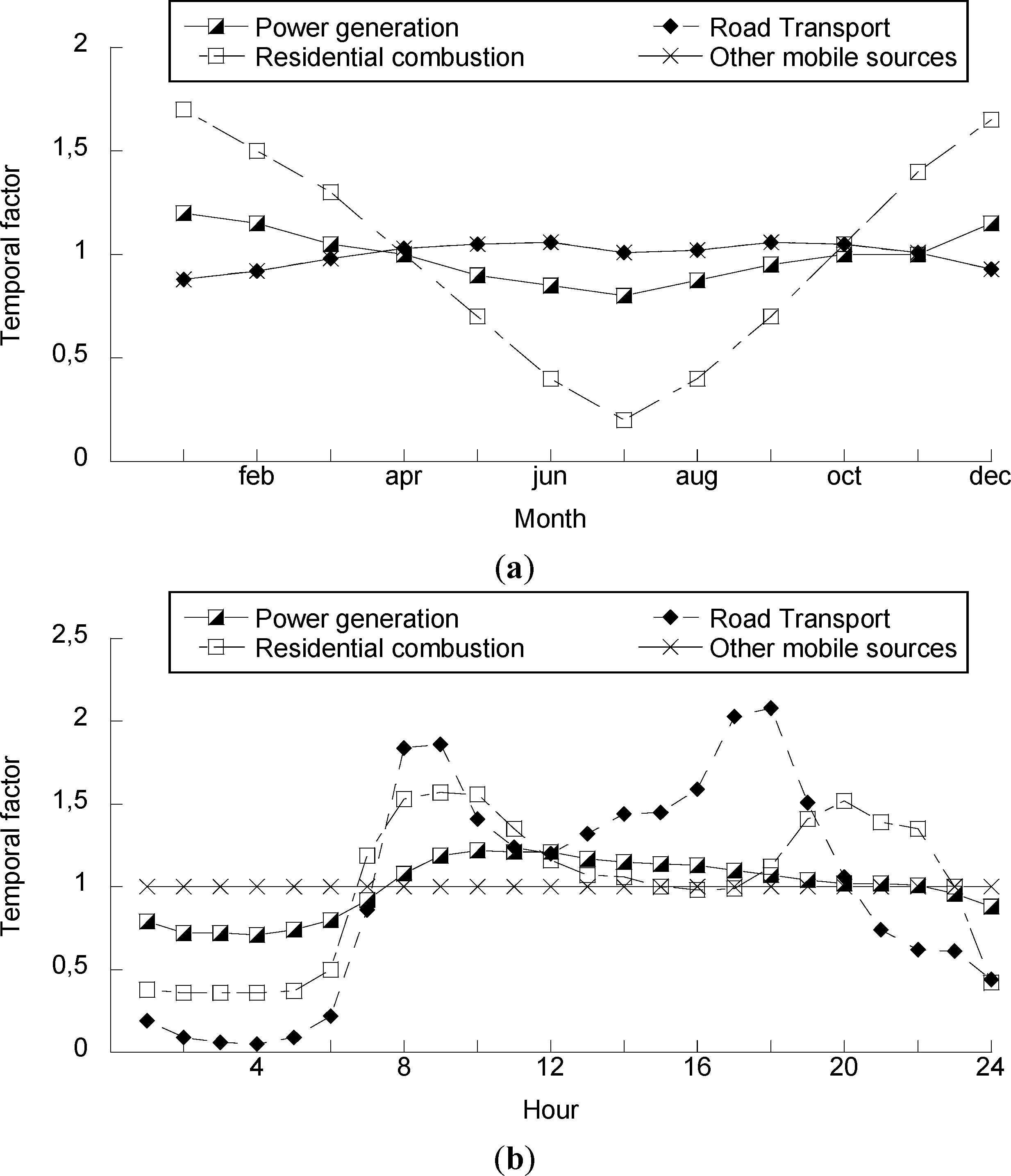
The temporal variation of the emissions is represented by monthly, daily and hourly time factors for each source category [44]. Examples for these time profiles are shown in Figure 1, showing that the emission variability during a day can be large (e.g., for traffic). The emission height distribution for all source sectors follows the EURODELTA project approach [45]. These profiles are spatially non-variant. Biogenic Volatile Organic Compound (VOC) emissions are derived from a dataset with the distributions of 115 tree species [24]. In these simulations, soil NOx emissions and forest fire are omitted in LOTOS-EUROS.
2.3. Satellite Data
The OMI instrument is a nadir viewing, space-borne spectrometer that measures the solar radiation backscattered by the Earth’s atmosphere and surface. OMI (on board the Aura satellite, launched on July 2004) measures in the spectral range from 270 to 500 nm with a spectral resolution of about 0.5 nm, from which slant columns of O3, SO2, NO2 and HCHO can be retrieved [12]. Cloud pressure and cloud fraction are derived from the O2-O2 absorption feature at 477 nm. The 114° viewing angle of the telescope corresponds to a 2,600 km-wide swath on the surface, enabling a daily global coverage of its measurements. Its spatial resolution is 24 × 13 km2 in nadir and increases to 68 × 14 km2 at the swath edges (discarding the outer 4 pixels). Overpass time is around 13:30 local time. The tropospheric NO2 columns are taken from the Royal Dutch Meteorological Institute (KNMI) DOMINO (Dutch OMI NO2) product v1.02 [46]. For each pixel, the modeled columns are compared to the OMI-NO2 column retrievals. For this purpose, all columns that fall in a single grid cell are averaged. Modeled columns are calculated, accounting for the averaging kernel. The contribution of the upper troposphere was neglected. Using v1.02 is motivated by the fact that several teams [16,17], including ours [18], have used this version to estimate emission trends across Europe. Although DOMINO v2 has brought a number of updates, the choice of version effects the model validation (with v2 having ∼10% lower NO2 columns) only.
2.4. In Situ Data
Within Europe, a dense measurement network of in situ stations is present. European countries report their monitoring data to the air quality database (AirBase) of the European Environment Agency (EEA) [47]. The spatial resolution of the LOTOS-EUROS model is coarse compared to city/street scales and cannot resolve enhanced concentrations near local sources. Therefore, only stations with a data coverage above 80% flagged as rural were considered here. Note that the classification of the AIRBASE stations is currently quite subjective and ambiguous, so that wrongly classified stations are to be expected in the rural dataset [48]. A few stations provide very high annual mean concentrations. Here, we have excluded all stations with annual mean concentrations above 30 μg/m3. The limit was chosen to be well above the rural background levels in the Netherlands and Belgium (11–23 μg/m3), which is where OMI indicates the NO2 hotspot in Europe is located. Following the selection of rural stations, a further selection was made to limit the validation dataset to stations with an altitude below 700 m. As such, stations located on mountain tops are excluded from the comparison. In total, 256 stations were used for the operational validation, mostly located in Western Europe.
The conventional methodology to monitor NO2 within a network is using molybdenum oxide converters in combination with chemiluminescence analysis. Comparison of the concentrations from these instruments to more selective techniques, such as Tunable Infrared Laser Differential Absorption Spectroscopy (TILDAS) and Differential Optical Absorption Spectroscopy (DOAS) show a significant interference in the measurements using molybdenum oxide converters [49–51]. These studies show that the ambient NO2 concentration during afternoon hours could be overestimated by a factor of 2–4. This interference correlates well with non-NOx reactive nitrogen species (NOz), as well as with ambient O3 concentrations, indicating a high impact of the interference for aged air masses. Unfortunately, the NOz conversion in molybdenum oxide converters is not complete or well determined. The interference has complications for the validation of the modeled diurnal cycles, as the molybdenum converters underestimate the diurnal cycle, as the afternoon minimum in NO2 is not represented well.
3. Model Evaluation Results
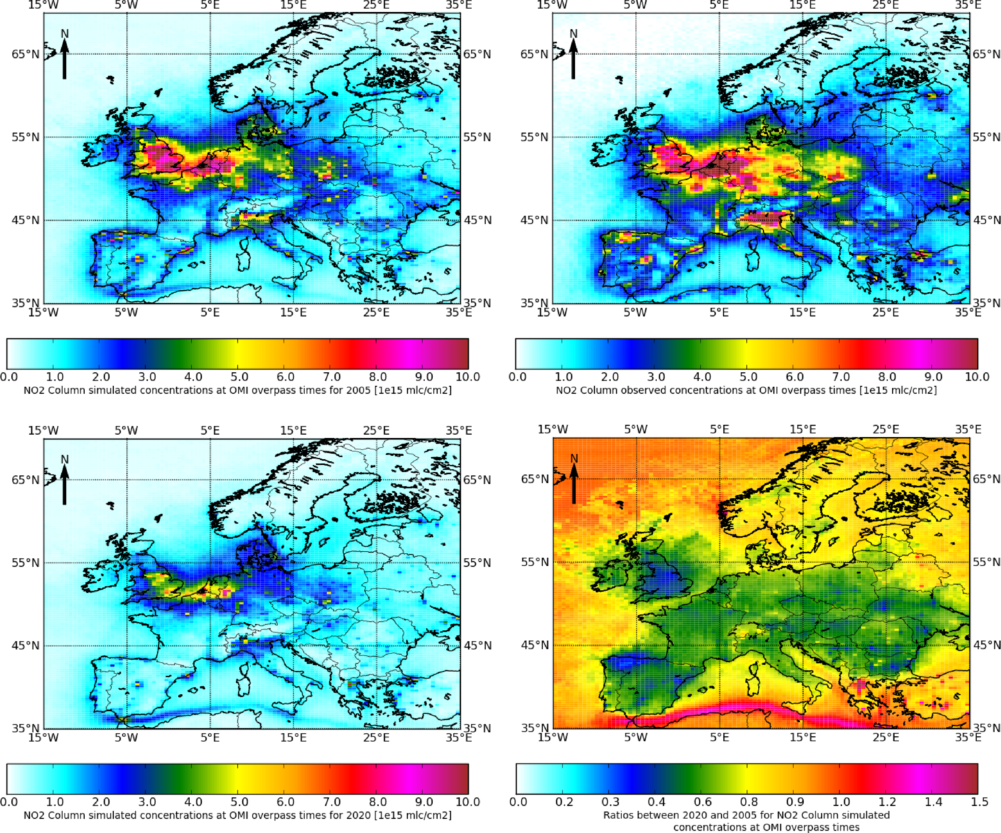
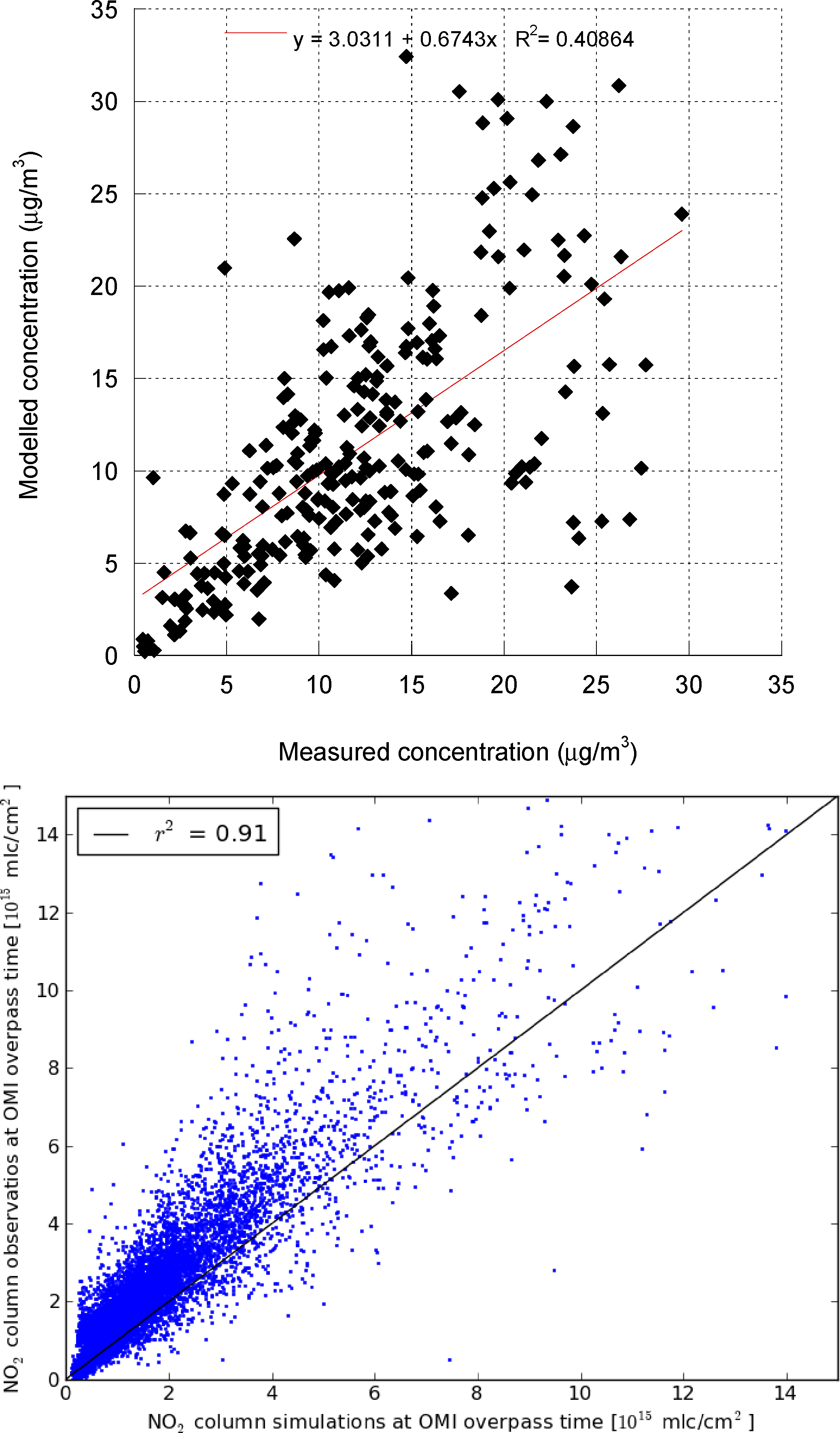
Prior to the presentation of the source apportionment results, we discuss the model performance for nitrogen dioxide. In Figure 2, the retrieved and modeled NO2 distribution are shown, respectively. Both show the highest column densities across the Benelux, Ruhr area, England, and the Po Valley. Many corresponding secondary maxima can be identified, including large cities (Paris, Barcelona and Istanbul) and industrialized areas (e.g., southern Poland, northern Spain and Marseille). In general, the modeled distributions shows many features and details that are also visible in the satellite retrievals, indicating that the model shows skill in capturing the spatial concentration distribution. The retrieved distribution is systematically higher than that modeled. Although the difference appears to be about 20% in the higher range (see Figure 3), one could also recognize a systematic difference of about 1 × 10¹⁵ mlc·cm−2 in the low range. The difference may be associated with systematic errors in the satellite retrievals, a contribution from the troposphere above 3.5 km, as well as uncertainties in the model parameterizations or emissions. All in all, the spatial correlation coefficient for the annual distribution indicated that the modeled distribution explains 91% of the variation in the OMI signal. This is very high for any air pollutant and demonstrates the skill of the LOTOS-EUROS model for this application. In Figure 4, time series for the area averaged the OMI-NO2 column across the Benelux and Poland are shown for the first half-year of 2005. The comparison shows that the model is able to reproduce the temporal behavior on a synoptic time scale. The model reproduces most features in the retrieved time series and captures the reduction in amplitude of the variability going from winter to summer. From March–April onwards, a systematic difference between retrieved and modeled columns is observed. This feature is present throughout the domain and prevails throughout the summer season. Hence, the systematic difference between retrieved and OMI annual means is derived from the summer season.
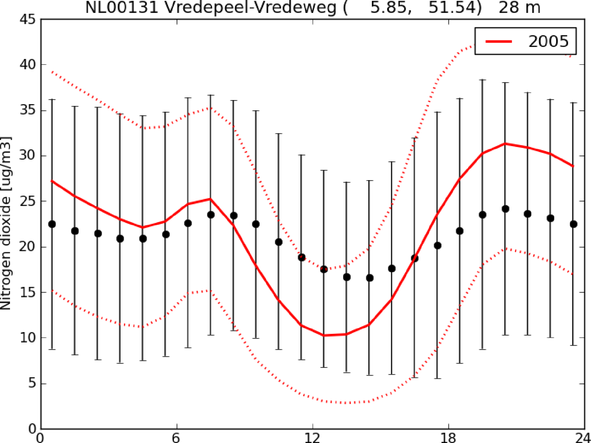
The modeled annual mean nitrogen dioxide concentrations are compared to those measured at the rural AIRBASE stations in Figure 3. Although the fit through zero has almost a slope of unity, the scatter (R2 = 0.41) for this comparison is considerably larger than for the comparison with OMI-NO2. First, the evaluation at ground level sites is more sensitive to mixing conditions than those for the column. Second, the NOz-artifact in the in situ monitors is variable in space and time with higher contributions in aged air masses and during the daytime. Finally, additional scatter is expected, due to siting issues and the impact of a variety of instruments and measurement procedures. The majority of the data points (86%) are within a factor two of the observed concentrations. Most of the stations outside this range are found on the low side, indicating observed concentrations to be underestimated. This feature was expected for stations that may be less representative for a model grid cell, such as stations in valleys or stations with impacts of local sources. However, most of the stations that are underestimated by more than a factor of two are located in Southern Europe. This may indicate that the NOz artifact of the monitoring instruments is relatively larger in Southern Europe, as NOz levels are higher, due to higher temperatures and radiation levels. Moreover, Southern Europe is characterized by more complex terrain and meteorology than Western and Central Europe. Secondary impacts may be derived from less representative emission information (e.g., time profiles). The statistical analysis also indicates a poorer model performance in Southern Europe than in Central and Western Europe (see Table 2). For instance, the average correlation coefficient at all stations is 0.6, whereas for the stations in Spain and Portugal, the values are considerably lower (<0.5). In contrast, the correlation coefficients for German, Belgian, Dutch and English stations are close to 0.7. The lower model performance for NO2 in Norway and Sweden can be explained by the low concentrations and low variability of concentrations. Figure 5 present an example of the validation of the diurnal cycle for NO2 at a regional station in the Netherlands (Vredepeel). It is observed that the model follows the cycle as seen in the measurements, albeit with a larger amplitude. This feature is observed for many sites.
The largest sink for nitrogen oxides is the chemical conversion to nitric acid and aerosol nitrate. Evaluation of the nitrate and total nitrate concentrations shows that the model underestimates their levels by about 25%–35% (not shown). Temporal correlations are generally between 0.6 and 0.7. For a detailed validation of LOTOS-EUROS for nitrate and nitric acid, we refer to Schaap et al. [52].
4. Source Apportionment
4.1. Present Day: 2005
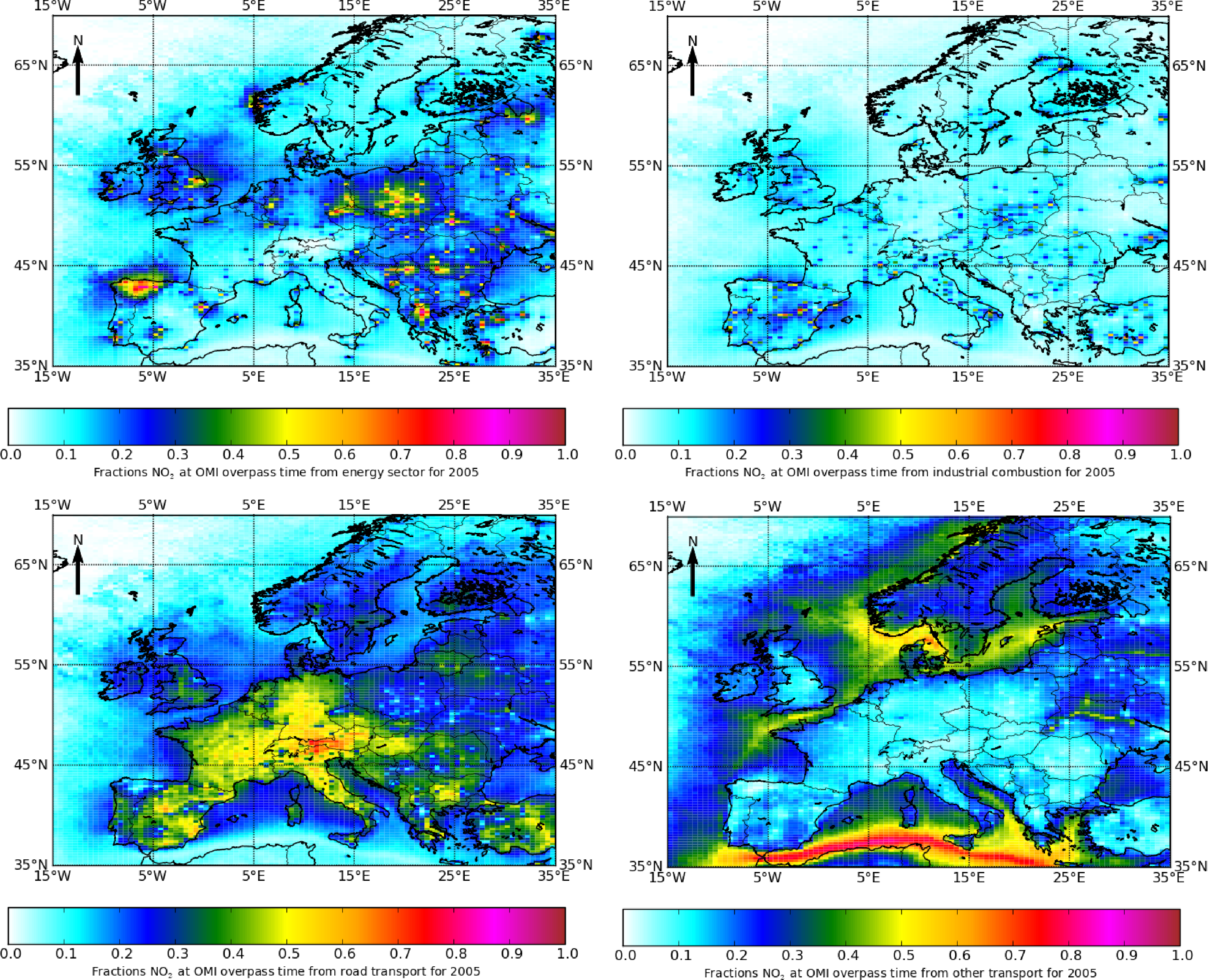
In Figure 6, we provide the sector contribution to the modeled OMI-NO2 column density. The most important contribution in Western Europe is made by road transport. On average, about 35% of the column is explained by road traffic. Across large parts of Germany and France, this percentage is around 50%, and towards southern Germany and the alpine region, higher values are found. Note that the maximum across the Alps is associated with very low modeled and observed columns. Industrial combustion contributes about 10%–15%, with local maxima around sources. Power plants are an important contributor to the modeled OMI-NO2 column in Eastern and southeastern Europe, as well as northern Spain, with contributions ranging between 30% and 70% in areas with large power plants. In most counties in Eastern Europe, e.g., Poland, Czech Republic and Slovakia, the power sector contributes equally or more to the country average modeled column than road transport. The increasing importance of the power sector is clearly visible in the decline of the share of road transport in this area. Off-road transport contributes 10%–15% across most of continental Europe. However, across the shipping tracks, the OMI signal is dominated by the local source. The importance of shipping emissions is also visible in coastal areas of, e.g., the Netherlands, Denmark and Sweden, where off-road transport contributes between 20% and 40%. All other sectors contribute about 10% to the modeled OMI signal.
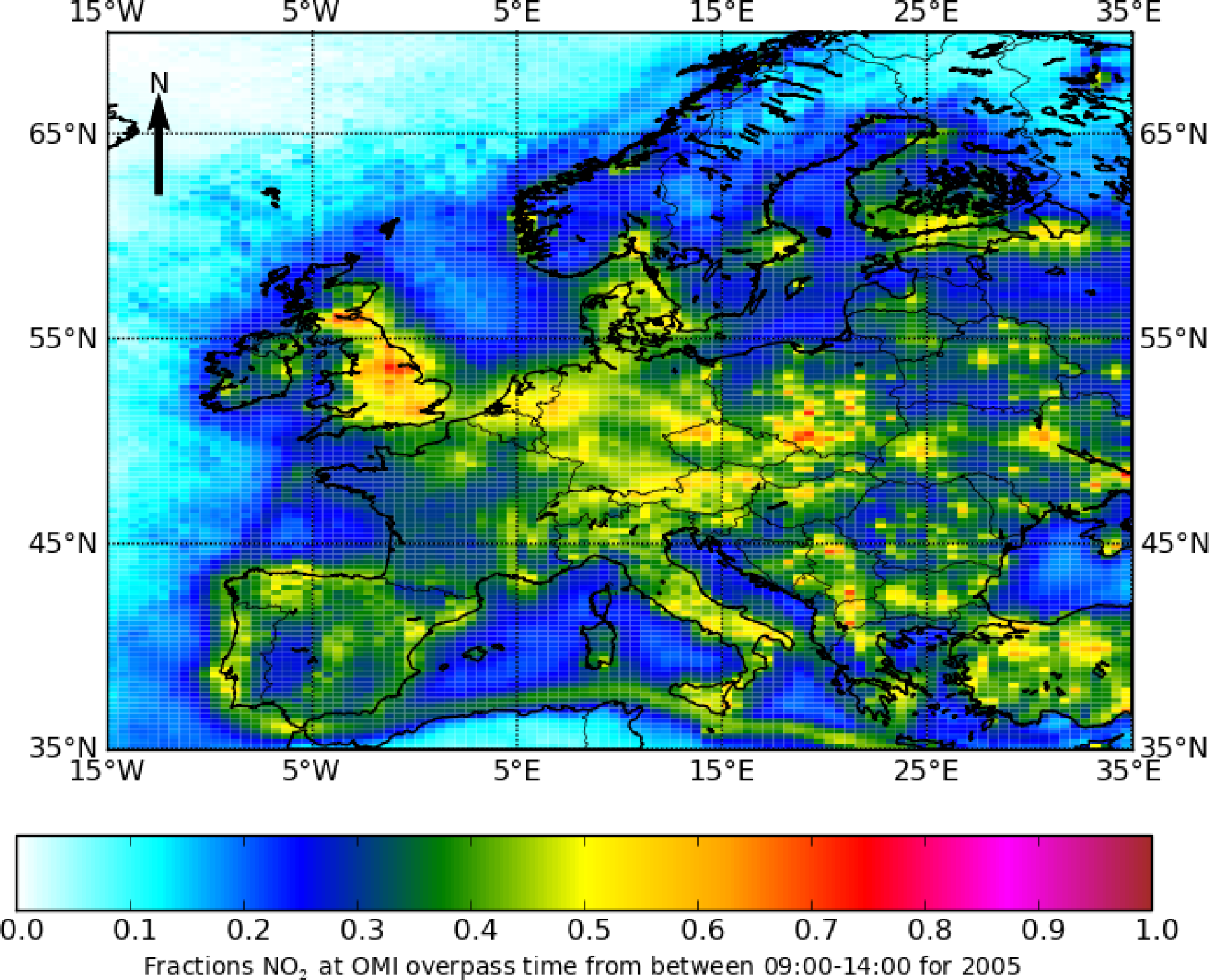
The sensitivity to the time of emission was also assessed. In Figure 7, we show the modeled OMI signal that is apportioned to the emissions from 09:00 till 14:00 local time. The distribution shows that in the source areas, this contribution is about 50%. Higher values are only observed near very large point sources. This value reduced towards 25% in rural areas of, for example, France, Spain and Eastern Europe. The only region with values below 20% is middle and northern Scandinavia. The distribution allows one to identify the regions that are more or less susceptible to long-range transport. Interestingly, the Po Valley, characterized by low ventilation, does not show up as a maximum, indicating that other factors are important, too. The exact reasons why OMI columns for some areas are more informative of recent emissions than for other regions is not easy to assess. Proximity to major sources, the height of the regional background, the dominant source sector and chemical lifetime and regime are likely to be key parameters. The source apportionment between sectors and hour of the day can be combined. For northern Spain and the Benelux, the structure of the hourly contributions is very similar in all sector contributions, indicating that the impact of different vertical emission structures does not affecting these results.
4.2. Future Situation: 2020
In Figure 2, the absolute distribution (lower left panel) and the ratio between 2020 and 2005 (lower right panel) is shown. The modeled reduction of NO2 columns across Europe in 2020 compared to 2005 is significant. Over most of continental Europe, the anticipated decline is about 30%–40%. The major emission reduction between 2020 and 2005 is expected for road transport and causes a decline in the apportioned column densities of a factor of about three. Furthermore, absolute power sector contributions are expected to decrease, but not as fast as the total, so that the relative share is expected to increase somewhat. Industrial combustion emissions and absolute contributions are forecasted to remain more or less stable. The largest expected reductions are observed over England, northern Spain and smaller areas in Eastern Europe, where local hotspots are present in 2005. These stronger than average declines, reaching 50%, are induced by reductions in the power sector on top of those in the road transport sector.
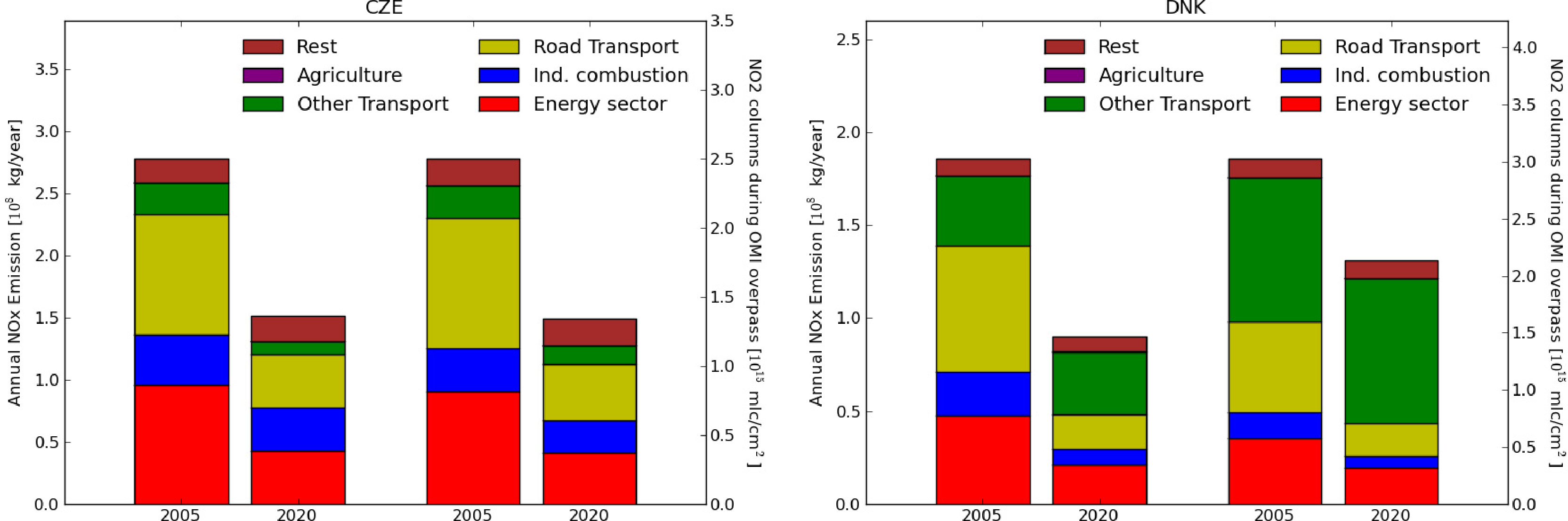
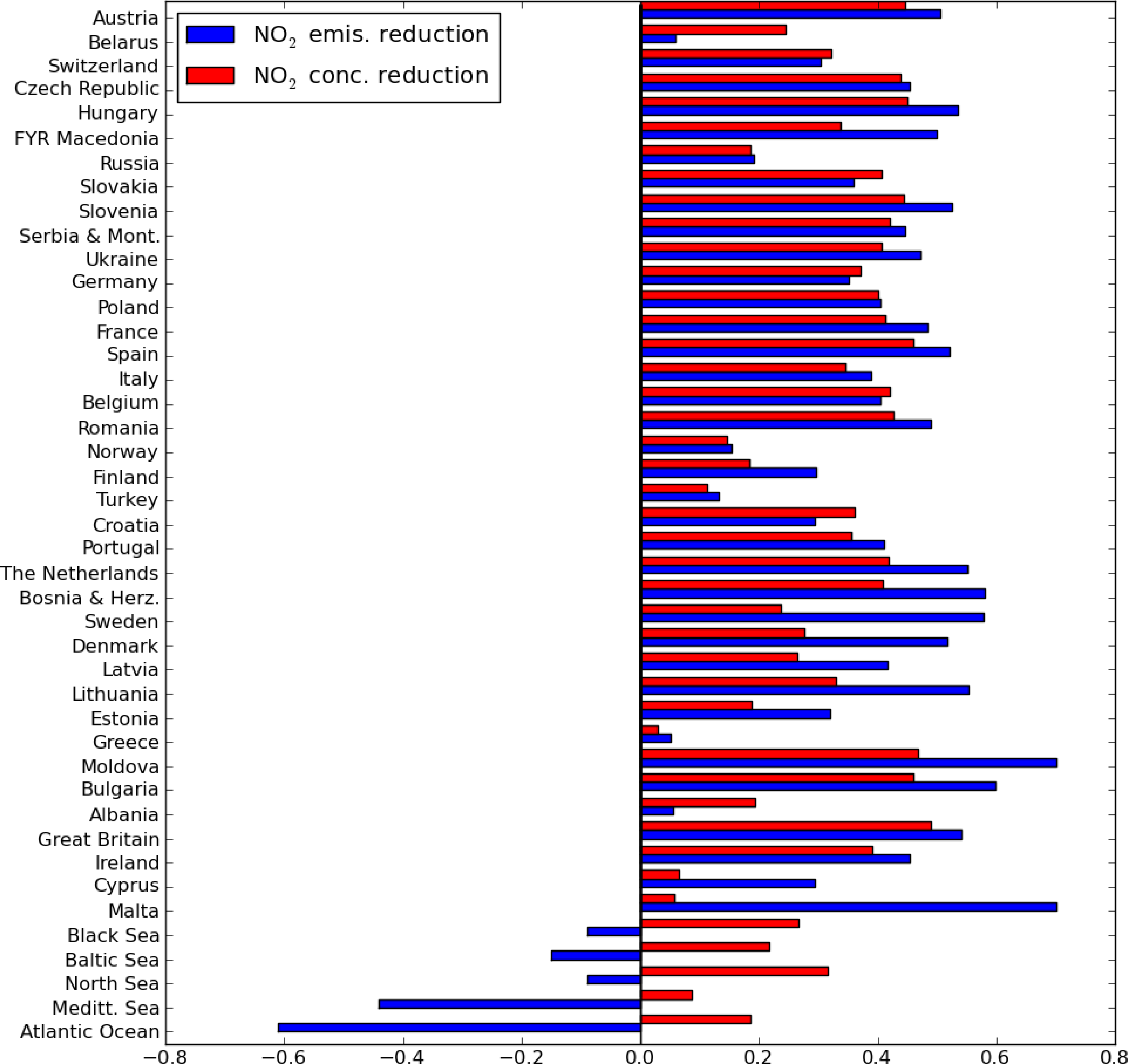
The only sector that is anticipated to grow significantly is off-road transport, more specifically shipping. This feature is visible in the shipping lanes. Shipping emissions significantly affect NOx columns above coastal areas. In these areas, the associated reduction in the NO2 columns may be on the order of 20%. In most of the coastal areas affected, the local emissions are decreased to a larger extent, but the increased transport of NOx from adjacent sea areas compensates for this partly. To illustrate this feature, we compare the expected emission change in Denmark to the modeled change in the NO2 column across the country in Figure 8(left). NOx emissions in Denmark are expected to halve in the 15 years under consideration. However, the modeled NO2 column reduces only by 25%, due to the increase of shipping emissions in the nearby seas. In contrast, the same comparison for a landlocked, continental country, like the Czech Republic, shows that the anticipated change in total emissions is reflected in the country averaged reduction in NO2 column values (see Figure 8(right)). To provide a bigger picture, we compare the expected relative change in national emission strength to that of the relative change in the modeled OMI-NO2 column across each nation in Figure 9. For large countries, as well as continental countries, the NO2 column reduction compares quite well to the emission reduction. However, for many middle-sized countries along a coast line, e.g., Sweden, Estonia and Lithuania, the same feature is observed as for Denmark, discussed above. In these countries, national efforts to reduce emissions are masked in the average reduction of the OMI-NO2 column by the impact of rising nearby shipping emissions. Cyprus is an exponent of this feature.
Furthermore, some other small countries show large deviations. This is expected, as their diameter is smaller than or comparable to the transport distance corresponding to the lifetime of NOx. Hence, they are more influenced by emissions in neighboring countries. Across the seas, the emission increases are visible in the ship tracks, but spatially averaged across their full size, the seas also show a decline in the NO2 column, as the outflow from the continent onto the sea areas declines. Note that in most countries, the emission reduction is slightly larger than the modeled change in the average NO2 column. This feature may be associated with a change in the lifetime of NO2 in the two scenarios. Indeed, the sensitivity of the satellite to emissions between 09:00 and 14:00 becomes lower in the case of the 2020 simulation, indicating a longer lifetime. The 2020 simulation shows lower ozone and oxidant levels than that for 2005, which explain this feature.
5. Discussions
In this study, we have used the LOTOS-EUROS chemistry transport model equipped with a source apportionment module to investigate the sensitivity of the modeled NO2 column, sampled at the OMI overpass time and location and weighted by the OMI averaging kernel, to emission sources. For this purpose, the contribution of the most important source sectors for NOx were labeled and tracked throughout a model simulation for 2005. The most important contribution (∼35%) in Western Europe is made by road transport. Across large parts of Germany and France, this percentage was calculated to be around 50%. Off-road transport and industrial combustion contribute 10%–15% each across most of continental Europe. In Eastern Europe, power plants are an important contributor to the modeled OMI-NO2 column and of comparable magnitude as road transport. These results may enhance the interpretation of the OMI satellite data. For instance, a number of studies [16–18] have shown large reductions (∼10%/yr) in NO2 columns across northern Spain and have argued that these reductions might be caused by technological measures in power plants. Our simulations clearly illustrate the dominant source contribution (60%–80%) of the power sector in this region, supporting the analysis that the power sector is the only sector able to cause such large reductions in NO2 columns. The emission control measures on the Spanish power plants have been implemented in 2008 and are also included in the emission estimates for 2020. In the scenario results, the impact of the change is obvious and of similar magnitude as reported. Likewise, we expect that major emission changes of power plants in Eastern Europe through modernization or fuel shifts will be visible in the OMI-NO2 column trends.
A number of studies have investigated the trends in OMI-NO2 columns using statistical techniques [16–18]. These studies interpret the trend in NO2 columns as an emission trend, neglecting the impact of transport on NO2 columns. We assessed the anticipated change in OMI-NO2 distributions between 2005 and 2020 to test if expected emission reductions could be traced by such an interpretation of the satellite data. The results indicated that for a large part of Europe, this in indeed possible. However, for medium- and small-sized coastal countries, the contribution of the expected increasing shipping emissions in adjacent sea areas may mask a significant part of the national emission reductions. Hence, for these countries, the trends of NO2 columns should be interpreted as a minimum. Note that there are also indications that secondary impacts through the change in chemical regime and, therefore, NOx lifetime may dampen the impact of an emission decrease slightly. In our simulations, almost all countries show a smaller reduction in NO2 columns than the expected reduction in emissions. This result should be taken with care, as this study did not include other impacts on oxidant levels across Europe, such as a steady increase in hemispheric background ozone concentrations [53] or potentially increased biological VOC emissions, due to climate change [54] or land use changes [24]. These issues highlight the need for a combined use of models, a priori emission estimates and satellite data to verify or falsify anticipated emission trends, e.g., [15,55,56].
The assessment of the source contributions can be further improved. The evaluation of the model results has shown that the model is capable of describing the spatial distribution of NO2 across Europe very well. We explain this feature by the relatively short lifetime of NOx in combination with the relatively well known emission distributions of NOx, including large point sources and traffic. However, the evaluation shows that the temporal behavior of the model can be improved. Important candidates for improvements are the functions to disaggregate the annual emission total into hourly emissions. These functions are overly simplified and have received little attention in the last few decades. The functions used are representative for Western European conditions and do not reflect differences in activity patterns, such as driving patterns or domestic heating in different parts of Europe. Shifts in these activity patterns on the order of 1–2 h may impact the bias between modeled and retrieved columns. Note that important factors affecting activity data, such as the impact of holidays, are not included. Combined with more complex terrain and variable meteorology, these shortcomings may explain the lower model performance for Southern Europe. Inversion studies using OMI data in combination with SCIAMACHY (SCanning Imaging Absorption spectroMeter for Atmospheric CHartographY) data may contribute to the evaluation of the diurnal emission pattern [57]. In short, an important improvement may be associated with improved representation of the emission variability. These improvements may also benefit the assessments made for secondary components, such as ozone and particulate nitrate, as well as nitrogen deposition.
Despite these shortcomings in the model and the emission description, we would argue that our modeling results are state-of-the-art. Comparison of the LOTOS-EUROS model performance for NO2 (as well as other components) shows that the model performs equally or better to comparable systems, such as EMEP, CHIMERE and RCG [28–30]. Moreover, the LOTOS-EUROS model shows a larger explained variability for OMI-NO2 columns compared to an ensemble of global and regional air quality presented in Huijnen et al. [58]. The deviations in the tropospheric NO2 columns of the individual ensemble models were on average in the range of 20–34% in the winter and up to 62% in the summer. Hence, the bias observed for LOTOS-EUROS is a general feature among current CTMs.
A potential explanation for the increased bias in NO2 columns during summer may be the lack or underestimation of soil-derived nitrogen oxide emissions. Based on an analysis of OMI data, Boersma et al. [59] suggested that the Yienger and Levy parameterization [60] for soil NOx emissions used in many models might be too low. New estimates for soil NOx emissions are considerably higher than before [61] and may help to close the gap between modeled and retrieved NO2 columns. A higher importance of soil NOx would complicate the assessment of anthropogenic emission trends from satellites further. Firstly, they would provide a background NO2 column, resulting in another cause why column trends could not be interpreted as emission trends. Moreover, due to the complex dependence on fertilizer use, this background would be dependent on agricultural practices and potential future shifts therein. It is planned to include the latest description of soil NOx emissions into LOTOS-EUROS to investigate if these emissions are realistic and to investigate how far they contribute to the OMI-signal.
In short, the OMI-NO2 columns can be a valuable data set to monitor air quality across Europe. We have shown how several sectors contribute to the OMI-NO2 signal across Europe. Furthermore, interpretation of a future trend in retrieved column densities as an emission trend needs to be addressed with care. Instead, a combination with (inverse) modeling appears to be a very strong strategy to verify or falsify anticipated trends.
6. Conclusions
We have applied a chemistry transport model to investigate the sensitivity of the modeled NO2 column, sampled at the OMI overpass time and location and weighted by the OMI averaging kernel, to emission sources across Europe. The most important contribution (∼35%) in Western Europe is made by road transport. Off-road transport and industrial combustion each contribute 10%–15% across continental Europe. In Eastern Europe, power plant contributions are of comparable magnitude as those of road transport. To answer the question if the OMI-NO2 trends can be translated directly into emission changes, we assessed the anticipated changes in OMI-NO2 between 2005 and 2020. Although the results indicated that for many countries, it is indeed possible, for medium- and small-sized coastal countries, the contribution of the increasing shipping emissions in adjacent sea areas may mask a significant part of national emission reductions. This study highlights the need for a combined use of models, a priori emission estimates and satellite data to verify emission trends.
Acknowledgments
This study was conducted under the EU-FP7 project, “Energy Observation for monitoring and assessment of the environmental impact of energy use” (EnerGEO, grant agreement no.: 226364)), and the ESA project, GLOB-EMISSION (grant number AO/1-6721/11/I-NB). The DOMINO data product was taken from the ESA TEMIS archive ( www.temis.nl) maintained at KNMI, The Netherlands.
Conflict of Interest
The authors declare no conflict of interest.
References
- Crutzen, P.J. The role of NO and NO2 in the chemistry of the Troposphere and Stratosphere. Ann. Rev. Earth Planet. Sci 1979, 7, 443–472. [Google Scholar]
- Sunyer, J.; Spix, C.; Quénel, P.; Ponce-de-León, A.; Pönka, A.; Barumandzadeh, T.; Touloumi, G.; Bacharova, L.; Wojtyniak, B.; Vonk, J.; et al. Urban air pollution and emergency admissions for Asthma in four European Cities: The APHEA Project. Thorax 1997, 52, 760–765. [Google Scholar]
- Searl, A. A Review of the Acute and Long Term Impacts of Exposure to Nitrogen Dioxide in the United Kingdom; Research Report TM/04/03; Institute of Occupational Medicine: Edinburgh, UK, 2004. [Google Scholar]
- Van Dingenen, R.; Dentener, F.J.; Raes, F.; Krol, M.C.; Emberson, L.; Cofala, J. The global impact of ozone on agricultural crop yields under current and future air quality legislation. Atmos. Environ 2009, 43, 604–618. [Google Scholar]
- Solomon, S.; Portmann, R.W.; Sanders, R.W.; Daniel, J.S.; Madsen, W.; Bartram, B.; Dutton, E.G. On the role of nitrogen dioxide in the absorption of solar radiation. J. Geophys. Res. D: Atmos 1999, 104, 12047–12058. [Google Scholar]
- Schaap, M.; Müller, K.; Ten Brink, H.M. Constructing the European aerosol nitrate concentration field from quality analysed data. Atmos. Environ 2002, 36, 1323–1335. [Google Scholar]
- Ten Brink, H.M.; Kruisz, C.; Kos, G.P.A.; Berner, A. Composition/size of the light-scattering aerosol in the Netherlands. Atmos. Environ 1997, 31, 3955–3962. [Google Scholar]
- Bobbink, R.; Hornung, M.; Roelofs, J.G.M. The effects of air-borne nitrogen pollutants on species diversity in natural and semi-natural European vegetation. J. Ecol 1998, 86, 717–738. [Google Scholar]
- Schöpp, W.; Amann, M.; Cofala, J.; Heyes, C.; Klimont, Z. Integrated assessment of European air pollution emission control strategies. Environ. Model. Softw 1999, 14, 1–9. [Google Scholar]
- Tørseth, K.; Aas, W.; Breivik, K.; Fjeraa, A.M.; Fiebig, M.; Hjellbrekke, A.G.; Lund Myhre, C.; Solberg, S.; Yttri, K.E. Introduction to the European Monitoring and Evaluation Programme (EMEP) and observed atmospheric composition change during 1972–2009. Atmos. Chem. Phys 2012, 12, 5447–5481. [Google Scholar]
- Burrows, J.P.; Weber, M.; Buchwitz, M.; Rozanov, V.; Ladstätter-Weißenmayer, A.; Richter, A.; Debeek, R.; Hoogen, R.; Bramstedt, K.; Eichmann, K.-U.; et al. The Global Ozone Monitoring Experiment (GOME): Mission concept and first scientific results. J. Atmos. Sci 1999, 56, 151–175. [Google Scholar]
- Levelt, P.F.; Van Den Oord, G.H.J.; Dobber, M.R.; Mälkki, A.; Visser, H.; de Vries, J.; Stammes, P.; Lundell, J.O.V.; Saari, H. The ozone monitoring instrument. IEEE Trans. Geosci. Remote Sens 2006, 44, 1093–1100. [Google Scholar]
- Bovensmann, H.; Burrows, J.P.; Buchwitz, M.; Frerick, J.; Noël, S.; Rozanov, V.V.; Chance, K.V.; Goede, A.P.H. SCIAMACHY: Mission objectives and measurement modes. J. Atmos. Sci 1999, 56, 127–150. [Google Scholar]
- Van der A., R.J.; Eskes, H.J.; Boersma, K.F.; van Noije, T.P.C.; van Roozendael, M.; de Smedt, I.; Peters, D.H.M.U.; Meijer, E.W. Trends, seasonal variability and dominant NOx source derived from a ten year record of NO2 measured from space. J. Geophys. Res. D: Atmos 2008, 113, D04302. [Google Scholar]
- Konovalov, I.B.; Beekmann, M.; Richter, A.; Burrows, J.P.; Hilboll, A. Multi-annual changes of NOx emissions in megacity regions: Nonlinear trend analysis of satellite measurement based estimates. Atmos. Chem. Phys 2010, 10, 8481–8498. [Google Scholar]
- Zhou, Y.; Brunner, D.; Hueglin, C.; Henne, S.; Staehelin, J. Changes in OMI Tropospheric NO2 columns over Europe from 2004 to 2009 and the influence of meteorological variability. Atmos. Environ 2012, 46, 482–495. [Google Scholar]
- Curier, R.L.; Kranenburg, R.; Segers, A.J.; Timmermans, R.M.A.; Schaap, M. Synergistic use of LOTOS-EUROS and OMI-NO2 Tropospheric Columns to evaluate the NOx emission trends across Europe. Atmos. Environ. 2013. Submitted. [Google Scholar]
- Castellanos, P.; Boersma, K.F. Reductions in Nitrogen Oxides over Europe driven by environmental policy and economic recession. Sci. Reports 2012, 2, 265. [Google Scholar]
- Russell, A.R.; Valin, L.C.; Cohen, R.C. Trends in OMI NO2 observations over the United States: Effects of emission control technology and the economic recession. Atmos. Chem. Phys 2012, 12, 12197–12209. [Google Scholar]
- Beirle, S.; Boersma, K.F.; Platt, U.; Lawrence, M.G.; Wagner, T. Megacity emissions and lifetimes of Nitrogen Oxides probed from space. Science 2011, 333, 1737–1739. [Google Scholar]
- Beirle, S.; Platt, U.; Wenig, M.; Wagner, T. Weekly cycle of NO2 by GOME measurements: A signature of anthropogenic sources. Atmos. Chem. Phys 2003, 3, 2225–2232. [Google Scholar]
- Pouliot, G.; Pierce, T.; Denier van der Gon, H.; Schaap, M.; Moran, M.; Nopmongcol, U. Comparing emission inventories and model-ready emission datasets between Europe and North America for the AQMEII Project. Atmos. Environ 2012, 53, 4–14. [Google Scholar]
- Manders, A.M.M.; Schaap, M.; Hoogerbrugge, R. Testing the capability of the chemistry transport model LOTOS-EUROS to forecast PM10 levels in the Netherlands. Atmos. Environ 2009, 43, 4050–4059. [Google Scholar]
- Beltman, J.B.; Hendriks, C.; Tum, M.; Schaap, M. The impact of large scale biomass production on ozone air pollution in Europe. Atmos. Environ 2013, 71, 352–363. [Google Scholar]
- Schaap, M.; Van Loon, M.; Ten Brink, H.; Dentener, F.J.; Builtjes, P. Secondary inorganic aerosol simulations for Europe with special attention to nitrate. Atmos. Chem. Phys 2004, 4, 857–874. [Google Scholar]
- Schaap, M.; Timmermans, R.M.A.; Roemer, M.; Boersen, G.A.C.; Builtjes, P.J.H.; Sauter, F.J.; Velders, G.J.M.; Beck, J.P. The LOTOS-EUROS Model: Description, validation and latest developments. Int. J. Environ. Pollut 2008, 32, 270–290. [Google Scholar]
- Curier, R.L.; Timmermans, R.; Calabretta-Jongen, S.; Eskes, H.; Segers, A.; Swart, D.; Schaap, M. Improving ozone forecasts over Europe by synergistic use of the LOTOS-EUROS chemical transport model and in situ measurements. Atmos. Environ 2012, 60, 217–226. [Google Scholar]
- Solazzo, E.; Bianconi, R.; Vautard, R.; Appel, K.W.; Moran, M.D.; Hogrefe, C.; Bessagnet, B.; Brandt, J.; Christensen, J.H.; Chemel, C. Model evaluation and ensemble modelling of surface-level ozone in Europe and North America in the context of AQMEII. Atmos. Environ 2012, 53, 60–74. [Google Scholar]
- Van Loon, M.; Vautard, R.; Schaap, M.; Bergström, R.; Bessagnet, B.; Brandt, J.; Builtjes, P.; Christensen, J.H.; Cuvelier, C.; Graff, A. Evaluation of long-term ozone simulations from seven Regional Air Quality Models and their ensemble. Atmos. Environ 2007, 41, 2083–2097. [Google Scholar]
- Vautard, R.; Builtjes, P.H.J.; Thunis, P.; Cuvelier, C.; Bedogni, M.; Bessagnet, B.; Honoré, C.; Moussiopoulos, N.; Pirovano, G.; Schaap, M.; et al. Evaluation and intercomparison of ozone and PM10 simulations by several Chemistry Transport Models over four European Cities within the CityDelta Project. Atmos. Environ 2007, 41, 173–188. [Google Scholar]
- Solazzo, E.; Bianconi, R.; Pirovano, G.; Matthias, V.; Vautard, R.; Moran, M.D.; Appel, K.W.; Bessagnet, B.; Brandt, J.; Christensen, J.H. Operational model evaluation for particulate matter in Europe and North America in the context of AQMEII. Atmos. Environ 2012, 53, 75–92. [Google Scholar]
- Stern, R.; Builtjes, P.; Schaap, M.; Timmermans, R.; Vautard, R.; Hodzic, A.; Memmesheimer, M.; Feldmann, H.; Renner, E.; Wolke, R. A model inter-comparison study focussing on Episodes with elevated PM10 concentrations. Atmos. Environ 2008, 42, 4567–4588. [Google Scholar]
- Thunis, P.; Rouil, L.; Cuvelier, C.; Stern, R.; Kerschbaumer, A.; Bessagnet, B.; Schaap, M.; Builtjes, P.; Tarrason, L.; Douros, J. Analysis of model responses to emission-reduction scenarios within the CityDelta Project. Atmos. Environ 2007, 41, 208–220. [Google Scholar]
- Walcek, C.J. Minor flux adjustment near mixing ratio extremes for simplified yet highly accurate monotonic calculation of tracer advection. J. Geophys. Res. D: Atmos 2000, 105, 9335–9348. [Google Scholar]
- Whitten, G.; Hogo, H.; Killus, J. The carbon bond mechanism for photochemical smog. Env. Sci. Techn 1980, 14, 14690–14700. [Google Scholar]
- Fountoukis, C.; Nenes, A. ISORROPIAII: A computationally efficient thermodynamic equilibrium model for K+-Ca2+-Mg2+-NH4+-Na+-SO42−-NO3−-Cl−-H2O aerosols. Atmos. Chem. Phys 2007, 7, 4639–4659. [Google Scholar]
- Banzhaf, S.; Schaap, M.; Kerschbaumer, A.; Reimer, E.; Stern, R.; Van Der Swaluw, E.; Builtjes, P. Implementation and evaluation of pH-dependent cloud chemistry and wetdeposition in the chemical transport model REM-Calgrid. Atmos. Environ 2012, 49, 378–390. [Google Scholar]
- Erisman, J.W.; Van Pul, A.; Wyers, P. Parametrization of surface resistance for the quantification of atmospheric deposition of acidifying pollutants and ozone. Atmos. Environ 1994, 28, 2595–2607. [Google Scholar]
- Simpson, D.; Fagerli, H.; Jonson, J.E.; Tsyro, S.; Wind, P.; Tuovinen, J.-P. Transboundary Acidification and Eutrophication and Ground Level Ozone in Europe: Unified EMEP Model Description; EMEP Status Report 1/03 Part I 2003; EMEP-MSC-West: Oslo, Norway, 2003. [Google Scholar]
- Kranenburg, R.; Segers, A.J.; Hendriks, C.; Schaap, M. Source apportionment using LOTOS-EUROS: Module description and evaluation. Geosci. Model Dev 2013, 6, 721–733. [Google Scholar]
- Wagstrom, K.M.; Pandis, S.N.; Yarwood, G.; Wilson, G.M.; Morris, R.E. Development and application of a computationally efficient particulate matter apportionment algorithm in a three-dimensional Chemical Transport Model. Atmos. Environ 2008, 42, 5650–5659. [Google Scholar]
- Kuenen, J.; Denier van der Gon, H.; Visschedijk, A.; van der Brugh, H.; van Gijlswijk, R. MACC European Emission Inventory for the Years 2003–2007; TNO Report TNO-060-UT-2011-00588; TNO: Utrecht, The Netherlands, 2011. [Google Scholar]
- Jozwicka, M.; JKuenen, J.P.; Denier van der Gon, H.A.C.; Visschedijk, A.J.H.; van Gijlswijk, R.N. Gridded Anthropogenic European Emission Data for the Base Year 2005 and Projection Years 2020, 2025 and 2030; TNO report TNO-060-UT-2012-01013; TNO: Utrecht, The Netherlands, 2012. [Google Scholar]
- Builtjes, P.J.H.; van Loon, M.; Schaap, M.; Teeuwisse, S.; Visschedijnk, A.J.H.; Bloos, J.P. Project on the Modelling and Verification of Ozone Reduction Strategies: Contribution of TNO-MEP; TNO-Report, MEP-R2003/166; TNO: Apeldoorn, The Netherlands, 2003. [Google Scholar]
- Cuvelier, C.; Thunis, P.; Vautard, R.; Amann, M.; Bessagnet, B.; Bedogni, M.; Berkowicz, R.; Brandt, J.; Brocheton, F.; Builtjes, P. CityDelta: A model intercomparison study to explore the impact of emission reductions in European cities in 2010. Atmos. Environ 2007, 41, 189–207. [Google Scholar]
- Boersma, K.F.; Eskes, H.J.; Veefkind, J.P.; Brinksma, E.J.; van der A, R.J.; Sneep, M.; van den Oord, G.H.J.; Levelt, P.F.; Stammes, P.; Gleason, J.F.; et al. Near-real time retrieval of Tropospheric NO2 from OMI. Atmos. Chem. Phys 2007, 7, 2103–2118. [Google Scholar]
- EEA. European Exchange of Monitoring Information and State of the Air Quality in 2005; ETC/ACC Technical Paper 2007/1; EEA: Copenhagen, Denmark, 2007. [Google Scholar]
- Joly, M.; Peuch, V.-H. Objective classification of air quality monitoring sites over Europe. Atmos. Environ 2012, 47, 111–123. [Google Scholar]
- Dunlea, E.J.; Herndon, S.C.; Nelson, D.D.; Volkamer, R.M.; San Martini, F.; Sheehy, P.M.; Zahniser, M.S.; Shorter, J.H.; Wormhoudt, J.C.; Lamb, B.K.; et al. Evaluation of nitrogen dioxide chemiluminescence monitors in a polluted urban environment. Atmos. Chem. Phys 2007, 7, 2691–2704. [Google Scholar]
- Steinbacher, M.; Zellweger, C.; Schwarzenbach, B.; Bugmann, S.; Buchmann, B.; Ordóñez, C.; Prevot, A.S.H.; Hueglin, C. Nitrogen oxides measurements at rural sites in Switzerland: Bias of conventional measurement techniques. J. Geophys. Res. D: Atmos 2007, 112, D11307. [Google Scholar]
- Villena, G.; Bejan, I.; Kurtenbach, R.; Wiesen, P.; Kleffmann, J. Interferences of commercial NO2 instruments in the urban atmosphere and in a smog chamber. Atmos. Meas. Tech. Discuss 2011, 4, 4269–4293. [Google Scholar]
- Schaap, M.; Otjes, R.P.; Weijers, E.P. Illustrating the benefit of using hourly monitoring data on secondary inorganic aerosol and its precursors for model evaluation. Atmos. Chem. Phys 2011, 11, 11041–11053. [Google Scholar]
- Stevenson, D.S.; Dentener, F.J.; Schultz, M.G.; Ellingsen, K.; van Noije, T.P.C.; Wild, O.; Zeng, G.; Amann, M.; Atherton, C.S.; Bell, N.; et al. Multimodel ensemble simulations of present-day and near-future tropospheric ozone. J. Geophys. Res. D: Atmos 2006, 111, D08301. [Google Scholar]
- Jacob, D.J.; Winner, D.A. Effect of climate change on air quality. Atmos. Environ 2009, 43, 51–63. [Google Scholar]
- Stavrakou, T.; Müller, J.-F.; Boersma, K.F.; De Smedt, I.; van der A, R.J. Assessing the distribution and growth rates of NOx emission sources by inverting a 10-year record of NO2 satellite columns. Geophys. Res. Lett 2008, 35, L10801. [Google Scholar]
- Konovalov, I.B.; Beekmann, M.; Richter, A.; Burrows, J.P. Inverse modelling of the spatial distribution of NOx emissions on a continental scale using satellite data. Atmos. Chem. Phys 2006, 6, 1747–1770. [Google Scholar]
- Boersma, K.F.; Jacob, D.J.; Eskes, H.J.; Pinder, R.W.; Wang, J.; van der A, R.J. Intercomparison of SCIAMACHY and OMI Tropospheric NO2 Columns: Observing the diurnal evolution of chemistry and emissions from space. J. Geophys. Res. D: Atmos 2008, 113, D16S26. [Google Scholar]
- Huijnen, V.; Eskes, H.J.; Poupkou, A.; Elbern, H.; Boersma, K.F.; Foret, G.; Sofiev, M.; Valdebenito, A.; Flemming, J.; Stein, O.; et al. Comparison of OMI-NO2 tropospheric columns with an ensemble of global and European Regional Air Quality Models. Atmos. Chem. Phys 2010, 10, 3273–3296. [Google Scholar]
- Boersma, K.F.; Jacob, D.J.; Bucsela, E.J.; Perring, A.E.; Dirksen, R.; van der A, R.J.; Yantosca, R.M.; Park, R.J.; Wenig, M.O.; Bertram, T.H.; et al. Validation of OMI Tropospheric NO2 observations during INTEX-B and application to constrain NOx emissions over the Eastern United States and Mexico. Atmos. Environ 2008, 42, 4480–4497. [Google Scholar]
- Yienger, J.J.; Levy, H., II. Empirical model of global soil-biogenic NOx emissions. J. Geophys. Res 1995, 100, 11447–11464. [Google Scholar]
- Hudman, R.C.; Moore, N.E.; Mebust, A.K.; Martin, R.V.; Russell, A.R.; Valin, L.C.; Cohen, R.C. Steps towards a mechanistic model of global soil Nitric Oxide emissions: Implementation and space based-constraints. Atmos. Chem. Phys 2012, 12, 7779–7795. [Google Scholar]


| EU-27 | Germany | Poland | Romania | Spain | Ukraine | |
|---|---|---|---|---|---|---|
| 1. Energy generation | 2.428 (22%) | 285 (19%) | 297 (41 %) | 101 (33%) | 336 (22%) | 390 (33%) |
| 2. Residential sector | 719 (6%) | 101 (7%) | 51 (7%) | 15 (5%) | 27 (2%) | 70 (6%) |
| 3. Industrial combustion | 1.593 (14%) | 68 (5%) | 99 (14%) | 42 (14%) | 345 (23%) | 152 (13%) |
| 4. Production processes | 227 (2%) | 94 (6%) | 8 (1%) | 13 (4%) | 10 (1%) | 41 (3%) |
| 5. Extraction of fossil fuels | 30 (0%) | 0 (0%) | 0 (0%) | 1 (0%) | 5 (0%) | 0 (0%) |
| 6. Solvent use | 0 (0%) | 0 (0%) | 0 (0%) | 0 (0%) | 0 (0%) | 0 (0%) |
| 7. Road transport | 4.428 (40%) | 656 (45%) | 176 (24%) | 107 (35%) | 527 (35%) | 264 (22%) |
| 8. Off-road transport | 1.547 (14%) | 178 (12%) | 88 (12%) | 27 (9%) | 228 (15%) | 263 (22%) |
| 9. Waste treatment | 31 (0%) | 0 (0%) | 0 (0%) | 0 (0%) | 3 (0%) | 0 (0%) |
| 10. Agriculture | 188 (2%) | 86 (6%) | 0 (0%) | 4 (1%) | 17 (1%) | 2 (0%) |
| Total | 11.190 | 1.469 | 721 | 309 | 1.497 | 1.183 |
| Countries | Obs | Mod | N | Bias | MAE | RMSE | Cor |
|---|---|---|---|---|---|---|---|
| Austria | 13.1 | 10.1 | 25 | □2.94 | 6.13 | 8.32 | 0.64 |
| Belgium | 18.5 | 19.7 | 10 | 1.20 | 6.98 | 8.74 | 0.67 |
| Switzerland | 18.2 | 9.9 | 7 | □8.20 | 10.71 | 13.59 | 0.60 |
| Czech Rep. | 13.4 | 11.3 | 12 | □2.17 | 4.81 | 6.51 | 0.63 |
| Germany | 12.1 | 12.3 | 56 | 0.14 | 4.87 | 6.36 | 0.68 |
| Denmark | 8.9 | 14.8 | 3 | 5.94 | 7.03 | 8.76 | 0.52 |
| Spain | 8.0 | 7.5 | 22 | □0.49 | 4.89 | 6.36 | 0.39 |
| Finland | 2.9 | 2.8 | 6 | 0.45 | 2.25 | 2.63 | 0.70 |
| France | 15.3 | 10.1 | 29 | □5.22 | 7.54 | 9.50 | 0.66 |
| Great Britain | 9.8 | 14.1 | 13 | 4.28 | 5.75 | 7.20 | 0.71 |
| Italy | 17.2 | 13.0 | 15 | □4.27 | 8.62 | 11.18 | 0.46 |
| Netherlands | 18.7 | 21.4 | 20 | 2.71 | 6.69 | 8.34 | 0.71 |
| Norway | 0.8 | 1.3 | 4 | 0.44 | 0.83 | 1.24 | 0.32 |
| Poland | 7.9 | 6.5 | 11 | □1.47 | 3.76 | 4.93 | 0.55 |
| Portugal | 5.2 | 4.7 | 6 | □0.51 | 3.21 | 4.04 | 0.17 |
| Sweden | 3.4 | 8.7 | 4 | 5.25 | 5.60 | 6.65 | 0.53 |
| All stations | 12.2 | 11.2 | 256 | □0.92 | 5.71 | 7.36 | 0.60 |
© 2013 by the authors; licensee MDPI, Basel, Switzerland This article is an open access article distributed under the terms and conditions of the Creative Commons Attribution license ( http://creativecommons.org/licenses/by/3.0/).
Share and Cite
Schaap, M.; Kranenburg, R.; Curier, L.; Jozwicka, M.; Dammers, E.; Timmermans, R. Assessing the Sensitivity of the OMI-NO2 Product to Emission Changes across Europe. Remote Sens. 2013, 5, 4187-4208. https://0-doi-org.brum.beds.ac.uk/10.3390/rs5094187
Schaap M, Kranenburg R, Curier L, Jozwicka M, Dammers E, Timmermans R. Assessing the Sensitivity of the OMI-NO2 Product to Emission Changes across Europe. Remote Sensing. 2013; 5(9):4187-4208. https://0-doi-org.brum.beds.ac.uk/10.3390/rs5094187
Chicago/Turabian StyleSchaap, Martijn, Richard Kranenburg, Lyana Curier, Magdalena Jozwicka, Enrico Dammers, and Renske Timmermans. 2013. "Assessing the Sensitivity of the OMI-NO2 Product to Emission Changes across Europe" Remote Sensing 5, no. 9: 4187-4208. https://0-doi-org.brum.beds.ac.uk/10.3390/rs5094187