3D Modeling of Coarse Fluvial Sediments Based on Mobile Laser Scanning Data

 , ,
, ,
Abstract
: High quality sedimentary measurements are required for studying fluvial geomorphology and hydrological processes e.g., flood and river dynamics. Mobile laser scanning (MLS) currently provides the opportunity to achieve high precision measurements of coarse fluvial sediments in a large survey area. Our study aims to investigate the capability of single-track MLS data for individual particle-based sediment modeling. Individual particles are firstly detected and delineated from a digital surface model (DSM) that is generated from the MLS data. 3D MLS points of each detected individual particle are then extracted from the point cloud. The grain size and the sphericity as well as the orientation of each individual particle are estimated based on the extracted MLS points. According to the evaluations conduced in the paper, it is possible to detect and to model sediment particles above 63 mm from a single-track MLS point cloud with a high reliability. The paper further discusses the strength and the challenges of individual particle-based approach for sedimentary measurement.1. Introduction
Acquisition of high precision and high-resolution topographical and sedimentary data is crucial for fluvial processes and hydraulic modeling. The sediment particle size and shapes are among the determining factors of fluvial geomorphology.
Laser scanning (LS) technology provides high-precision and high resolution three-dimensional (3D) topographical information, which allows more advanced estimation of river bed roughness and grain size distribution. The capacity of the terrestrial laser scanning (TLS) for fluvial morphology has been studied by Hodge et al. [1]. TLS is further used for studying roughness patterns [2,3]. Surface based statistical approaches have been applied to determine grain size [4] and surface sedimentology [5] by analyzing the local standard deviation of raw TLS point clouds or TLS produced digital surface models (DSM). Accurate surface roughness data derived from TLS are used as input data in computational fluid dynamics (CFD) [6]. However, data acquisition with TLS is limited to a plot scale survey range and limits a synoptic understanding of a larger study area. Furthermore, although TLS is capable of offering high precision 3D information at the single particle scale, an individual particle-based approach for sedimentary measurements from TLS data has thus far rarely been applied.
High resolution (cm-mm level) mobile laser scanning (MLS) nowadays enables studies on highly detailed terrain features in a large surveying range. MLS was first introduced to fluvial research using a boat-based mobile mapping system (BoMMS) in Alho et al. [7]. The creation of the BoMMS system intrigues the adoption of MLS in fluvial studies, but the use of MLS for measuring river bed morphology, roughness, and surface sedimentology is still in its early stages due to the lack of automated processing and analysis algorithms of the hundreds of gigabyte data generated [8]. Since the MLS technology has advanced into the cm to sub-cm resolution, it is now possible to detect and to extract individual sediment particles from the MLS point cloud. If individual particles can indeed be automatically detected and extracted from MLS point cloud data, this will open the gate to acquiring more detailed sedimentary information (e.g., size, orientation, sphericity and roundness of each particle) in large areas, which could bring the quantity and quality of particle size measurements and surface roughness estimation beyond the current state of the art.
The main objective of this paper is to conduct a baseline evaluation on the capacity of recent MLS technology for individual particle-based sediment modeling. Section 2 introduces the “Akhka” backpack MLS system that is applied to collect the single-track MLS data that is used for the individual particle detection and modeling. An automated 3D modeling process is developed to detect and to extract individual particles from the MLS raw point cloud, and to estimate the size, sphericity and orientation of each detected particle based on the extracted MLS points. The 3D modeling process is an iterative process combining three different approaches, namely: (1) the detection of individual particles from a digital surface model (DSM) generated from the MLS raw point cloud; (2) the delineation of the 2D boundary and extraction of MLS points of each detected individual particles; and (3) the estimation of the particle size, sphericity and orientation based on the extracted MLS points of each particle. The computational algorithms of the three approaches are presented in Section 3. The results of the particle size estimation from the MLS data are compared with the field measurements. The capacity of the single-track MLS data for individual particle detection and modeling as well as the advantages and challenges of the individual particle-based process for sedimentary measurements are discussed in Section 4 of the paper.
2. Data Acquisition and Preprocessing
2.1. Study Site and Data Collection
2.1.1. “Akhka” Backpack MLS System
Backpack-based platforms [9,10] are designed to meet the challenges set by the terrains and environments that are hard to access for typical MLS platforms such as vehicles, UAVs and helium-balloons. In this study, a MLS system called “Akhka” is applied to collect the sedimentary information on the gravel bar in the study site.
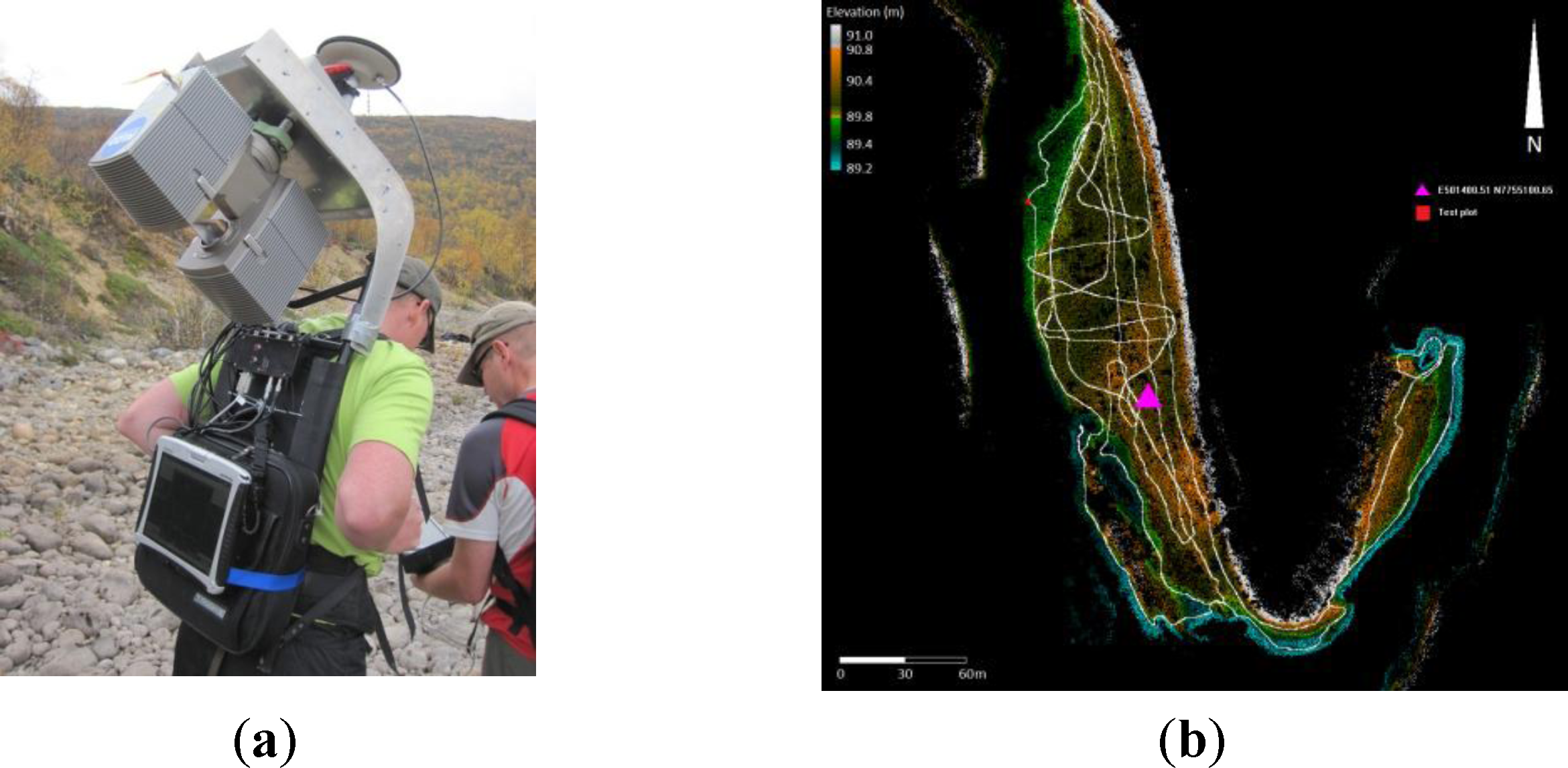
The laser scanning unit in Akhka is a FARO Photon 120 that uses a 785 nm laser with a power of 20 mW. The laser beam diameter at the scanner is 3.3 mm and the beam spreads according to a 0.16 mrad divergence angle, which results a 20 mm laser footprint at 100 m from the scanner. The highest available angular resolution with a scanning frequency of 48 Hz is 0.3 mrad (0.018°) with PRF of 976 kHz, which produces a 6 mm point spacing of adjacent points in a scan profile at the typical range of 20 m. This is sufficient for 3D modeling purposes at mm resolution level within the scan profile. The scanner head in Akhka was mounted directly under the IMU unit and when operated it pointed downwards roughly at an angle of 40 degrees to yield cross-track profiles (Figure 1a).
A NovAtel SPAN GPS-IMU set (NovAtel DL-4plus receiver and GPS-702 antenna, Honeywell HG1700 AG11 tactical-grade RLG IMU) is integrated into the platform. The Waypoint Inertial Explorer™ GPS-IMU post-processing software is applied to combine the reference station data with the GPS-IMU data collected by the SPAN equipment, and to calculate the survey track of the platform. The computed platform track (scanning track) together with the raw laser data and the system boresight calibration information are used to produce the 3D point cloud. Any noisy points were manually removed during the post processing of point cloud.
2.1.2. Study Site and Experimental Data
The study site is located in northern Finland on river Utsjoki, which is a tributary of the sub-arctic river Tana that forms part of the border between Finland and Norway. The river is usually covered by ice from November to April. The normal annual discharges on the study reach vary between 25 and 120 m3·s−1 and the water level rises several meters during the spring flood due to snow melt. Particle size on the river bed varies mostly from sand to fine gravel, and from coarse gravel to cobble and even boulders on the floodplain. The floodplain is almost entirely non-vegetated. These fluvial-geomorphological characteristics make the river Utsjoki a favorable area to undertake sediment modeling.
The MLS measurement was conducted in an area of 50 m × 100 m on a gravel bar of the Utsjoki River in September of 2011 when the water level was at its lowest and the gravel bar was accessible. The data acquisition was carried out with 49 Hz scan frequency and 244 kHz point measurement rate. The platform speed is below 4 km·h−1. Data was recorded in blocks of 1,500 profiles, with a total of 106 blocks. Eight spherical targets were located in the test area and registered with RTK-GPS in order to evaluate the geometric quality of the MLS point cloud data. According to the accuracy analysis reported in Kukko et al. [9], comparing the RTK-GPS measured and the MLS system measured locations of the eight spherical targets, the 2D RMSE (Root Mean Square Error) for all the targets was 18 mm in the horizontal plane and 29 mm in elevation, the 3D RMSE for the targets was 34 mm. The absolute accuracy of the MLS point cloud data is 17 mm–23 mm regarding both (x, y) plane and elevation. The point density over the test area varies from 1,800 pts·m−2 to 50,000 pts·m−2, with the mean point density being 9,100 pts·m−2.
During the same day as the MLS data collection, after the scan, 150 sediment particles were randomly selected from a 1.4 m × 1.4 m (2 m2) plot in the test area, the a- and b-axes of each selected particle were manually measured in the field, and the D50 in the plot is 70 mm. Since the main interest of this study is to investigate the potential of the single-track MLS data for individual particle-based sediment modeling, the MLS point cloud of the 2 m2 plot in which the manual grain size measurement was conducted is chosen as the experimental data. The entire MLS dataset of the test area and the location of the experimental data are illustrated in Figure 1b. The point cloud of the experimental data is presented in Figure 2a. There is no non-sediment object in the plot of the experimental data, and the plot is covered by a single scanning track. The total number of points in the plot is 32,907 pts, and the average point density is 1 pts·cm−2. The MLS points are heterogeneously distributed due to the influences from the platform speed, the scanning angle, the object surface orientation, and the object distance from the scanner. The maximum point spacing along the scan profile is about 3 mm and the minimum point spacing along the scan profile is about 1 mm, while the maximum profile spacing along-track is about 69 mm, and the minimum profile spacing is about 3 mm in the experimental data.
2.2. Generation of the DSM
The DSM referred to here is a raster that represents the earth’s surface and includes ground objects on it. Individual sediment particles on river point bars are recognizable in the DSM by human eyes when the resolution of the DSM reaches the cm level. We therefore assume that it should be possible to automatically detect individual particles from a high resolution DSM.
The DSM is generated from the MLS point cloud of the experimental data. Delaunay conforming triangulation [11] is applied to the MLS point cloud to create a triangulated irregular network (TIN) of the area. A natural neighbor interpolation [12] is then used to calculate a raster DSM from the TIN. Figure 2b shows the DSM generated from the MLS point cloud.
The detection of individual sediment particles requires a high resolution DSM, but the resolution of the DSM is constrained by the point density of the MLS data. Theoretically, the resolution of the DSM can reach the minimum point distance, which is 1 mm for the experimental data. However, the highest resolution is not necessarily optimal for sediment modeling due to the interpolation deformations. Since both the maximum point spacing along the scan profile and the minimum point spacing between scan profiles are about 3 mm, a resolution approximating to 3 mm is chosen to guarantee that there is at least one MLS point per pixel along the scan profiles, while one MLS point per pixel can also be expected along the direction of scanning track at the locations where the scan profiles are dense. According to the size of the experimental data and the requirement of a resolution of approximately 3-mm, a resolution of 3.2 mm is used for the final DSM calculation.
3. Methods
The process of individual particle-based sediment modeling from MLS data is divided into three different approaches: first, the individual particles must be detected and separated from each other, which is achieved by a segmentation of the DSM; secondly, the 2D boundary of each individual particle has to be delineated from the DSM segment, and the MLS points of the particle need to be extracted from the point cloud according to its 2D boundary; finally, the particle size, sphericity and orientation are estimated based on an ellipsoid model that is calculated using the extracted MLS points. Figure 3 illustrates the work flow of the process, which begins with larger particles, and iterates through the three approaches to extract smaller particles until most of the plot has been covered by the extracted individual particles. Computational algorithms applied for the above mentioned approaches are introduced in Sections 3.1, 3.2 and 3.4. Section 3.3 provides more details on the iterative process.
3.1. Detection of Individual Particles from the DSM Segmentation
The general concept of the DSM-based ground object detection is to segment the DSM according to the textural and morphological characteristics of the objects contained in the DSM. Considering the nature of the morphological features present by the sediment particles in the DSM, the classic digital image segmentation algorithm called Pouring is applied in order to isolate the individual particles. The DSM is smoothed and denoised before the segmentation to improve the outcome of the algorithm.
3.1.1. Morphological Smoothing and Denoising of the DSM
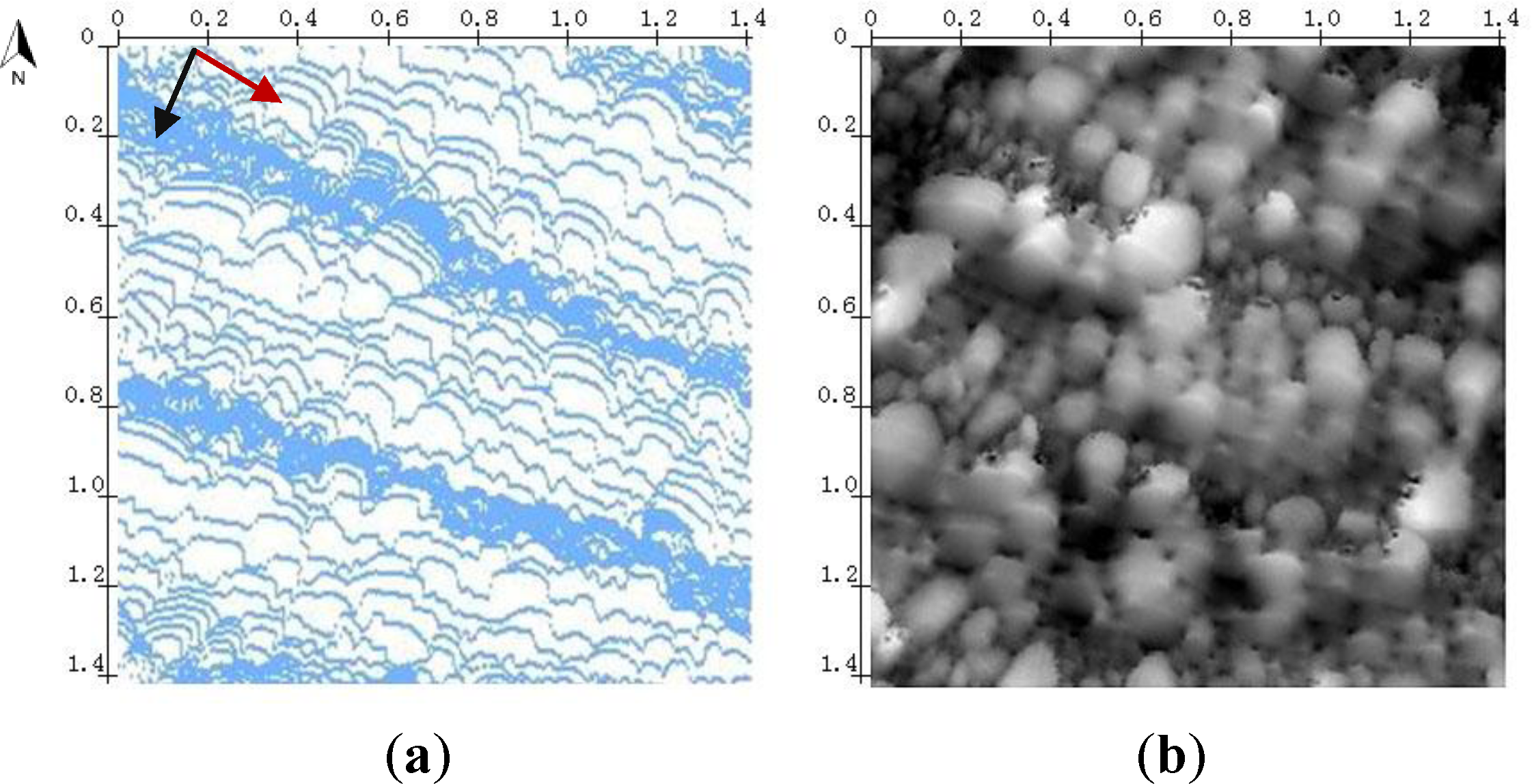
As shown in Figure 4a, due to the interpolations during the DSM generation, the sediment particles tend to present smooth boundaries in the DSM, while the heterogeneous distribution of MLS points produces bright undulations along the direction of the scan profile and dark holes along the scanning track direction, which requires smoothing and denoising of the DSM before segmentation. The challenge here is to find a good algorithm to clean the undulation and noises in the DSM, while keeping the boundaries of the particles intact. Instead of traditional isotropic diffusion algorithms such as Gaussian smoothing, morphological smoothing and denoising are chosen to fulfill the task.
The basic concept of morphological smoothing and denoising is to suppress the bright details smaller than a specified structuring element (SE) by Opening, and to suppress the dark details smaller than an SE by Closing [13]. The operation of Opening and Closing are different combinations of the basic morphological operations of Erosion and Dilation. The Erosion of a gray-scale image I with a gray-scale SE, noted as [I ⊕ SE], is defined as:
Erosion “darkens” the image in a general sense, namely, the bright features are reduced, dark features are thickened, and the background is darker, while Dilation presents the opposite effects. Erosion and Dilation by themselves are not very useful in terms of image processing, but these two basic operations become powerful when used in combination with higher-level processes such as Opening and Closing. The Opening of image I by SE is an Erosion followed by a Dilation, which can be noted as I ˚ SE = (I ⊖ SE) ⊕ SE, and the Closing of image I by SE is a Dilation followed by an Erosion, i.e., I • SE = (I ⊕ SE) ⊖ SE. A simple interpretation of Opening is that the operation smoothens the image at its peak regions (neighborhood of local maxima) with the structure element SE; peak regions smaller than SE will be smoothed, the remaining parts of the image remain intact. A similar interpretation for Closing is that it smoothens the basin regions (neighborhood of local minima) of an image, basins, or gaps smaller than SE will be filled up.
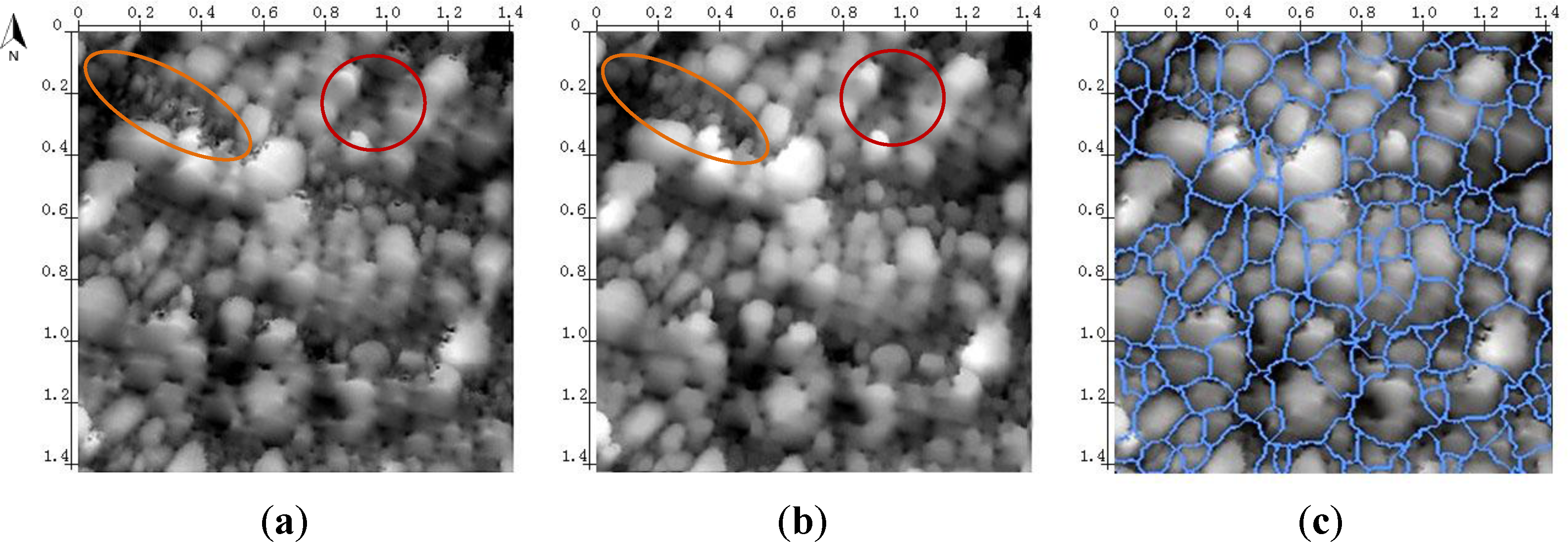
For the purpose of sediment particle segmentation, the bright undulations on the peaks of the DSM need to be smoothed and the dark holes at the basins should be eliminated. We use flat structure elements that are symmetrical, of unified intensity value and with the origin at the center for both Opening and Closing. An equilateral octagonal shape is applied to the structure elements to derive a suitable approximation for a circular structure. Since the average undulation width in the DSM is about 3 cm (10 pixels) and the average hole radius is about 1 cm (3 pixels), the structure element for Opening is larger (9 pixels in width and height) and the structure element for Closing is smaller (3 pixels in width and height). Figure 4b illustrates the results of the morphological Opening and Closing, in which, compared to the original DSM in Figure 4a, both undulations and holes are effectively smoothed, and the boundaries of sediment particles remain mostly untouched.
3.1.2. Morphological Pouring
Pouring regards the DSM as a “mountain range”. Larger intensity values correspond to mountain peaks, while smaller intensity values correspond to valley basins. Pouring segments the DSM in several steps. First, the local maxima are extracted, i.e., pixels that have larger intensity values than their immediate neighbors (in a 4-neighborhood). In the next step, a region expansion is simultaneously started from all the local maxima until “valley basins” are reached. The expansion is continued as long as there are chains of pixels in which the intensity value becomes smaller, just like water running downhill from the maxima in all directions. Points at valley basins are split amongst all neighboring segments in the last step. The Pouring is done by a uniform expansion of all the involved local maxima, until all ambiguous pixels are assigned. Pouring delivers a preliminary segmentation of individual particles. It can be assumed that there is at least one sediment particle inside each DSM segment. However, the boundaries of Pouring segments do not represent the boundaries of the sediment particles (Figure 4c). The boundary of the individual particles must be delineated more precisely so that the MLS points of the particles can be accurately extracted from the point cloud.
3.2. Delineation of Boundary of Individual Particles
Because the Pouring algorithm tends to firstly find the locally dominant regions (mountain), and to assign the pixels of the subordinate regions (valley basins) to the dominant regions, a DSM segment of the Pouring results usually consists of a dominant particle (the largest or highest particle in its local neighborhood) and several subordinate particles (smaller and lower particles in the neighborhood). The exact 2D boundary of the detected particle needs to be delineated from the DSM segment so that the MLS points of the detected particle can be extracted from the point cloud accordingly. The active contour model is used to delineate the boundary of the dominant sediment particle in a DSM segment of the Pouring result.
3.2.1. Active Contour and Curve Evolution
The active contour models, also called “Snakes”, are first described in Kass et al. [14] as a controlled continuity spline curve under the influence of image forces and external constraint forces. Since the original work of Kass et al. [14], the active contour has become one of the most powerful instruments for boundary detection. The basic concept of Snakes is to find salient image features such as edges, lines, and subjective contours through the motion of a spline curve (like a snake) that minimizes certain energy functionals of the curve. For a Snake, an energy functional describing the total energy of a curve in an image system is defined so that the total energy of the curve is reduced while the curve moves toward the desired features in the image. The curve is locked to the features once it touches them because the total energy of the curve is then minimized and there is no further force to move the curve anymore. The classic energy functional of a curve C is:
Since the energy functional depends on the parameterization of the curve and is not directly related to objects’ geometry, the classic model is non-intrinsic, and it is also not capable of handling change in the topology of the curve during its motion [15]. To improve the active contour models, Caselles et al. [15] proposed a geodesic approach of active contours that connects the classical energy based deformable spline curves to the geometric curve evolution, thereby leading to a great simplification of the formulation and the implementation of the active contour models.
For a curve C denoted as: C (p), p ∈ (0, 1), with C(0) = C(1) to close the curve, the evolution of the curve C is to deform C in time t by adding a velocity V to each point C (p) along C in the direction of the normal vector N⃗ of C (p):
As shown in Figure 5, if V equals the curvature k of the curve C, the evolution Ct = k · N⃗ is according to the “curvature flow” and it will smooth and compress the curve until it shrinks to a small circle. If an external constraint functional gI (C) is added, thus:
With a given image I, gI (C) can be considered as an energy functional of curve C in the image system I, the total energy of C can be describes as:
The task of the boundary detection by curve evolution can be interpreted as a gradient descent process of the energy functional gI (C), i.e., to deform the curve C until the total energy of C in the system of image I is reduced to the minima. The minimization of the functional gI (C) can be solved by deriving the Euler-Lagrange equation using calculus of variations. The Euler-Lagrange equation of gI (C) is described as the following:
The active contour models present their power especially when the desired feature presents noisy, segmented, or incomplete information in the image. The art of using active contours lies in the design of the gI function that is adapted to the different problems of feature delineation in 2D or even surface fitting in 3D spaces.
3.2.2. Delineation of Particle Boundary Using Active Contour without Edges
Most of the classical models of active contours rely on the edge-detectors depending on the image gradient ∇I to stop the curve evolution and, therefore, work well with those objects presenting high gradients at the boundaries. However, this is not the case for the sediment particles in the DSM. Because of the point density limitation of the single-track MLS data and the interpolation of the DSM generation, sediment particles tend to present very smooth features in the DSM, and the gradient at the grain boundaries can sometimes be even smaller than at other locations of the grain surface.
In this paper, we use an energy function that is not based on the gradient of the image, and the active contour model is called “Active Contour without Edges”. The energy function gI is according the Mumford-Shah functional [16] and the curve evolution is implemented using the level sets as described in [17].
A parametric spline curve C (p), p ∈ (0,1) can be represented implicitly via a function ϕ, by C = {(x,y)|ϕ (x,y) = 0}, i.e., ϕ = 0 at the location of curve C. The function ϕ is called a level set and it can be further formulated so that ϕ > 0 inside the region closed by curve C and ϕ < 0 outside the curve C (Figure 6).
Using the geometrical definition of the normal vector N⃗ and the curvature of k a curve, it can be proved that:
Using the level set ϕ, an energy function g in an image system I is designed based on the variance of the image values I (x,y) inside the curve Varin and the variance of I (x,y) outside the curve Varout. Taking a binary image as an example, the values inside the boundary of an object are 1 while the value outside the object are 0, Varin + Varout of a curve in the image is equal to 0 only when the curve is located at the boundary of the object. For any other image, Varin + Varout ≈ 0 when the curve locates at the boundary of the object. The energy functional g is:
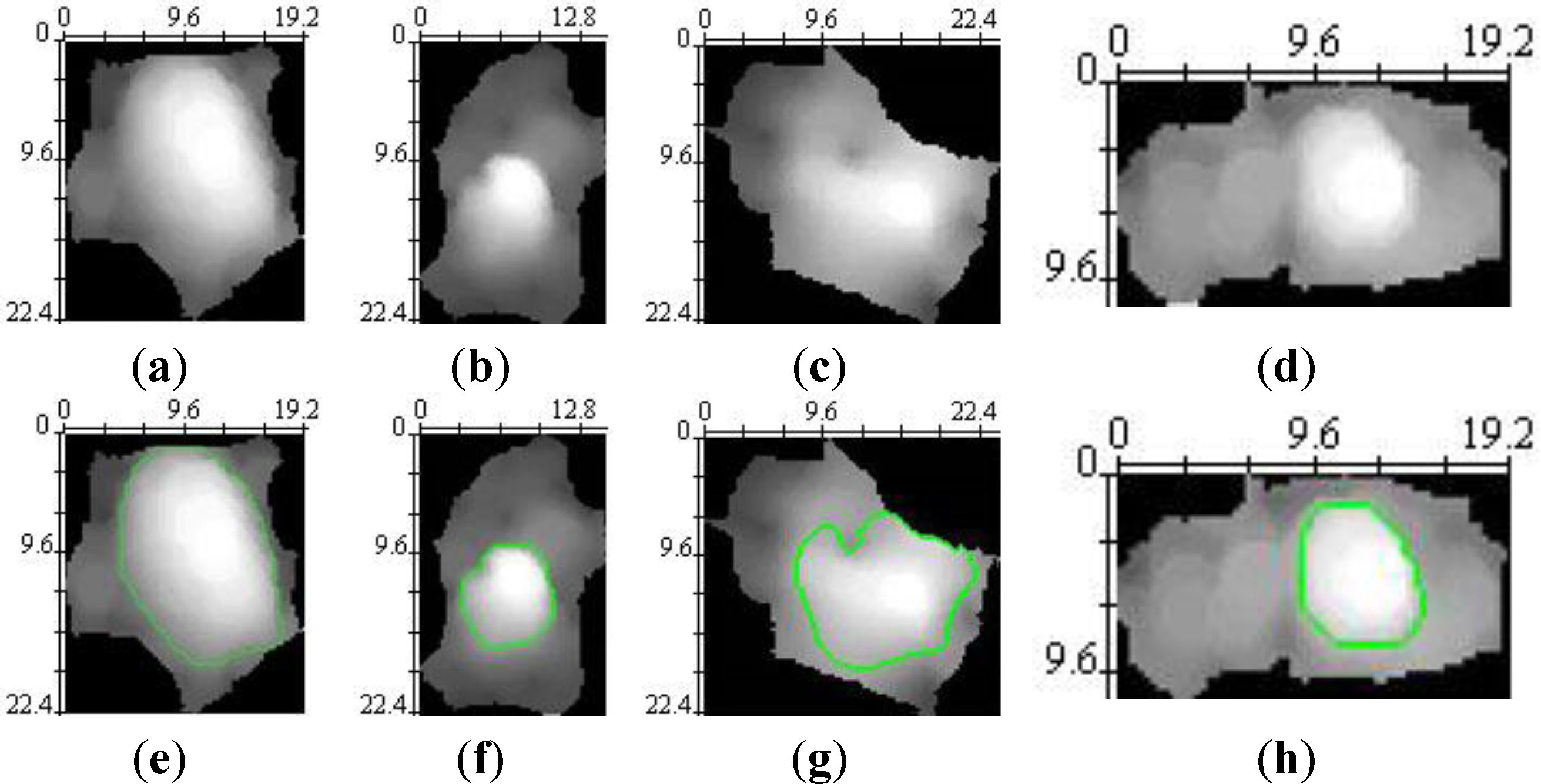
We follow the algorithm of Chan et al. [17] for the implementation with the restriction that at most only one particle can be delineated in one DSM segment at one time. We therefore restrict the curve evolution by initializing the curve ϕ0(x,y) at the region of maximum in the DSM segment, and using the parameter setting as μ = 0.05•2552, λ1 = λ2 = 1. The parameter setting is to guarantee the continuity of the first derivative without requiring the continuity of the second derivative in order to allow concave bends and to prevent sharp corners on the curve, as well as to ensure only one object boundary can be delineated (to find the dominant particle in the segment) in the calculation. The curve evolution stops when CΔt is smaller than a 0.001 tolerance, which means the solution of the functional reaches to a stationary stage. Figure 7 shows some examples of the particle boundary delineation.
3.3. Iterative Approach
As mentioned in Section 3.2, the DSM segments derived by the Pouring algorithm usually contain more than one sediment particle. This fact can be easily recognized from the examples in Figure 7. The reason is that the Pouring algorithm only considers the most “competitive” single or group of local maxima as the starting points of its uniform expansion, which means that the algorithm selects the most dominant particle in a local neighborhood during the implementation in order to avoid an over-split of the DSM. It can be assumed that new local maxima will be found once the most “competitive” maxima, namely, the dominant particle are removed from the DSM.
According to the characteristics of the Pouring algorithm, it can be deduced that, (1) there is complete information of at least one dominant (larger or higher) sediment particle in a DSM segment of Pouring; (2) there can be complete and/or incomplete information of other neighboring subordinate (smaller or lower) sediment particles in a DSM segment; (3) once the information of the dominant sediment particles are removed from the DSM, it is possible to find other sediment particles by re-iterating the Pouring and the active contour algorithms on the updated DSM. During the boundary delineation, we use the initial curve and the parameter settings to restrict the active contour algorithm so that only the boundary of the dominant sediment particle can be delineated from one DSM segment. Once the exact boundaries of the dominant sediment particles are delineated, the information of those particles is removed from the DSM by replacing the intensity of the corresponding regions with a background intensity (e.g., 0). The Pouring algorithm is then re-iterated based on the updated DSM and the new segmentation results provide the information of other sediment particles that were subordinate in the previous calculation.
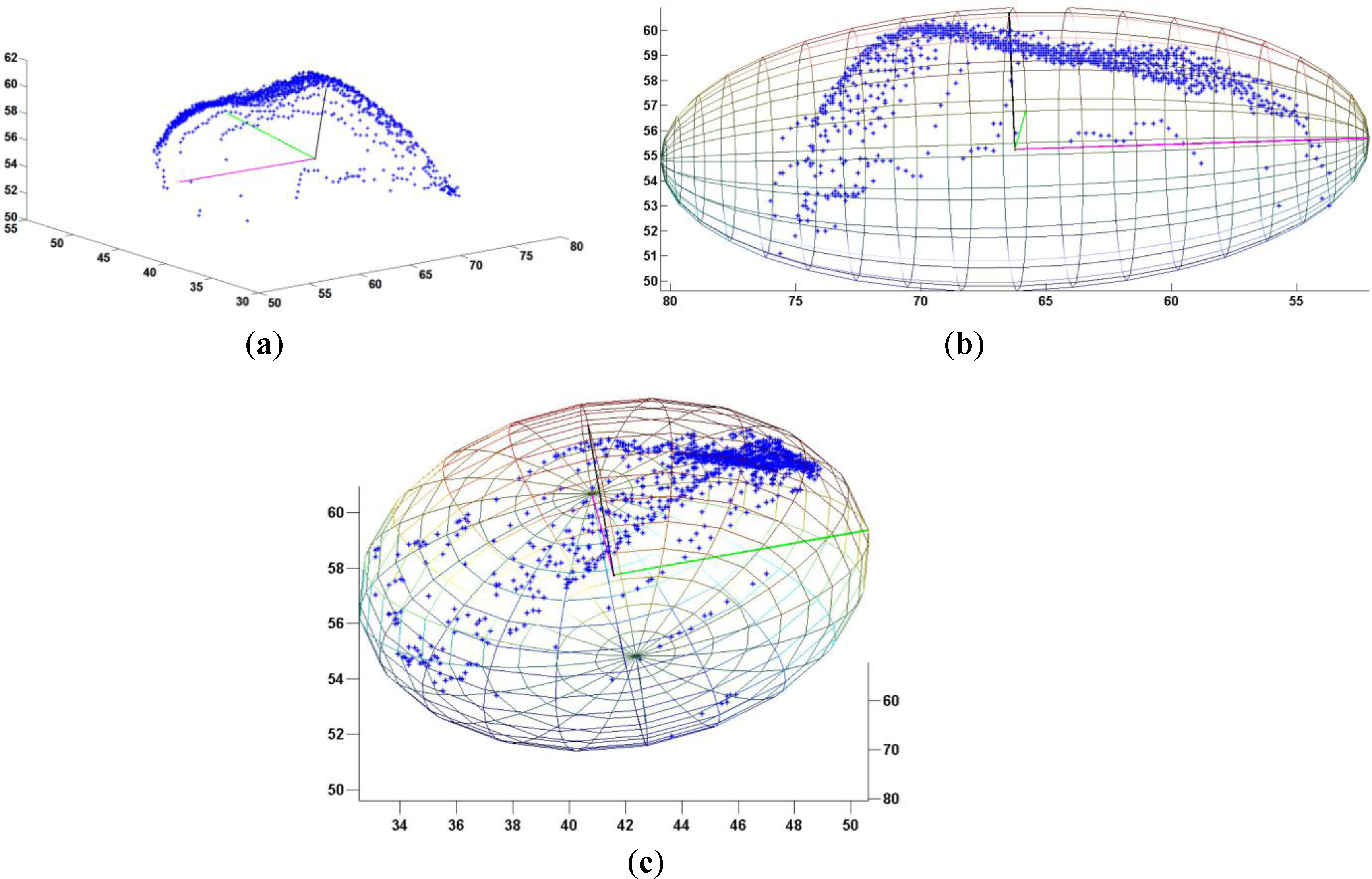
Following the workflow demonstrated in Figure 3, the process iterates through the particle detection (DSM segmentation with Pouring algorithm) and the particle extraction (boundary delineation with active contour algorithm), until a termination criterion is satisfied (e.g., 95% of the DSM area has been covered by the delineated particle contours). MLS points of each individual particle are extracted according to the 2D boundary of the particle. A minimum volume enclosing ellipsoid (MVE) is then fitted for each particle based on the extracted MLS points. The location of the center, the directions and length of the three axes, are calculated, and the sphericity of the particle is considered as the same as the sphericity of the ellipsoid.
3.4. Estimation of Particle Size, Sphericity and Orientation Based on Ellipsoid Model of MLS Points
MLS points of an individual particle can be extracted from the point cloud according to the x, y coordinates of the MLS points and the 2D boundary of the particle delineated from the DSM. The MLS points present the 3D shape information of an individual particle or at least the protrusion part of an individual particle. In the study at this stage, we use ellipsoid model to fit the MLS points in order to estimate the size (a-, b- and c-axes), the sphericity and the orientation of an individual particle or the part of an individual particle captured by the MLS system. The concept of the covariance matrix is employed for the ellipsoid fitting.
In statistics, for any given point set P in an assigned neighborhood, similarities between the points in the neighborhood can be found by means of the neighborhood’s covariance matrix M:
However, this theory only stands for an ideal setting that requires the points to be normally distributed in the neighborhood, which is hardly the case with real life MLS data. Due to the obvious non-normality and nonlinearity of the MLS points, the induced covariance matrix becomes unreliable. To optimize the ellipsoid fitting, a minimum volume enclosing ellipsoid (MVE) is calculated. The computing algorithm is described in Khachiyan et al. [18], which is an iterative solver to minimize log (det (A)) subjected to an arbitrarily oriented ellipsoid defined by the equation:
4. Results and Discussions
4.1. Results
The experiment data was processed by the algorithm with three iterations. Altogether 750 particles were found within the 2 m2 plot, beside two boulders, 22.8% of the found particles were cobbles, 63.87% were coarse gravels and 13.06% were medium gravels (Table 1).
A 2D sediment map is generated combining the 2D contours and the 3D geometric characteristics. Figure 9 shows the 2D map of the detected sediment particles. Since we stopped the iteration when 95% of the DSM had been delineated with individual particles, there is about 5% of non-segmented area (black regions in Figure 9d) in the DSM. These non-segmented areas consist of the un-delineated particles, gaps between particles and some errors (part of mistakenly delineated particles). After three iterations of the particle detection, it can be assumed that the particle size of the remaining un-delineated particles in the area will not surpass 63 mm. Technically the un-delineated particles in these areas can still be processed by another iteration, but we stopped the process because the reliability of the DSM segmentation and boundary delineation decreases as the number of iterations increases.
4.2. Discussion
4.2.1. Comparison with Field Measurement Results
At the time when the field work was conducted in September 2011, the most pressing issue was to test the operability of the Akhka backpack MLS system in fluvial environments where other platforms cannot be used due to mobility limitations, and to analyze the capacity (resolution and accuracy) of the 3D point cloud produced by the system under different scanning setting, terrain and object surface situations. The data collection was designed to meet the target of general performance evaluation of the MLS system rather than focusing on sedimentary measurements. A 1.4 m × 1.4 m (2 m2) plot was randomly chosen from the test area in the field and the a- and b-axes of 150 randomly selected particles in the plot were manually measured. The MLS data of the 2 m2 plot was selected as the experimental data for this study because it is the only place in the test area where valid field reference data is available. The field measured grain size distribution of the plot is listed in Table 2. Figure 10 illustrates the comparison of the grain size distribution measured based on single-track MLS data and in the field.
The comparison shows that the coarse gravel population of the MLS-based measurement (63.87%) is much higher than of the field measurement (33.41%), whereas the presence of cobble population in the MLS-based measurement (22.8%) is lower than in the field measurements (58.45%). The MLS-based measurement also provides a large population of medium gravel (13.06%), which disagrees markedly with the field measured result (0.48%).
However, as shown in Figure 10, the population distribution of the four grain sizes in the field measured data presents a high correlation to the area distribution of the four grain sizes in the MLS-based measurement. Although the areal coverage of coarse gravel from MLS measurement (33.41%) seems to be smaller than the population rate from the field (42%), it should be noticed that there is 4.75% of un-segmented area left in the MLS-based measurement, and as mentioned in Section 4.1, the particle size of the un-segmented area will not surpass 63 mm, thus, it can only belong to coarse, medium or even finer particles.
The presence of this kind of correlation is probably due to the result of the field measurements, which should ideally represent a random selection of sediment particles, but actually reflects the probability of a particle of a sediment class been selected from the plot rather than the population rate of the sediment class in the plot. However, the probability of a particle of a sediment class being selected is more likely determined by the areal coverage (e.g., the visibility to human eyes) of the sediment class in the plot. For example, despite the high population rate of the medium gravel (13.06%) in the MLS-based measurement, the actual areal coverage of medium gravel in the plot is only about 0.48%, and the visibility of the medium gravels is fairly low as shown in green in Figure 9d. Hence the chance for a medium gravel to be selected during the field measurement is limited by its low visibility in the plot. Therefore, we would assume that the grain size distribution according to population based on the MLS-based measurement is more relevant to the grain size distribution than the one measured in the field.
Since there is lack of one-to-one measurement records for the particles from the field reference data, the evaluation of the MLS-based results at this stage can only rely on the distribution of the grain size. According to the comparison between the MLS-based measurements and the field measurements, there is a high correlation between the field measured grain size distribution and the MLS-based grain size distribution when considering the areal coverage of different sediment classes. With the current valid reference information, it is impossible to evaluate whether an individual particle is correctly extracted or how precise the size, sphericity and orientation estimation of a specific particle is.
For a more rigorous validation of the individual particle-based sediment modeling process, we would propose a more sophisticated field measurement campaign that could provide one-to-one measurement records of the particles inside a test plot. Measured particles in the plot should be labeled. A photo of the whole scene would be needed to record the labels and locations of the measured particles. In order to reduce the impact of perspective distortion, the camera should be placed on a leveled stand and located in the center of the plot with the lens facing downwards to the ground, parallel to the surface. The particles should be labeled before the MLS data collection and measured after the MLS data collection so that the particle movements caused by the sediment measurements would not influence the results. If possible, TLS data should also be collected for the same test plot to serve as additional reference information for the evaluation of the performance conducted by the MLS system.
4.2.2. Impact Factors of the Performance
The most influential factor of the individual particle-based sediment modeling process is the density and the distribution of the MLS points.
The minimum detectable particle size is determined by the point density. The highest point density in the experimental data is 7 pts·cm−2, which means a 10 mm-size medium gravel can be described by more than five MLS points. With such a point density, there is almost 1 MLS point per pixel for the calculation of a DSM with 3.2 mm resolution. A 10 mm-size medium gravel will take at least 9 pixels on the DSM with little interpolation deformation, and therefore, could be detected by the algorithm. The lowest point density in the experimental data is 0.23 pts·cm−2, thus the calculation of the high resolution DSM (e.g., 3.2 mm) at those locations relied on interpolation, which leads to a strong smoothness of particle shapes in the DSM. Larger particles such as cobbles and boulders can be detected from the DSM, but the reliability of the estimation of the size and the orientation of particles at those locations is reduced because the point density controls the validity of the 3D shape of the particles. With an average 1 pts·cm−2 point density and a heterogeneous point distribution, the recent single-track MLS data can hardly capture sufficient surface details of a particle to support an analysis on the particle roundness. However, with the individual particle-based approach, it is possible to retrieve the 3D surface of a particle if the point density is high enough, and the particle roundness can be evaluated with surface-area measurement [20].
The point density of the MLS data is non-uniform due to the heterogeneous point distribution. The point distribution along the scan profile is determined by the scanning frequency of the laser equipment and the object distance from the scanner, while the point distribution along the scanning track is controlled by the platform speed. The experimental data of this study has 1–3 mm point spacing along the scan profile, and 3–69 mm profile spacing along the scanning track, which means that the plot is located within a 10 m range beside the scanning track, but not directly below the scanner. In order to derive a point density that is satisfactory for the detection of sediment particles above 20 mm (at least 1 pts·cm−2), we suggest that the target area should be within a 10 m range either side of the scanning track, and the platform speed (walking speed of the backpack carrier) should be kept as slow and even as possible.
Another potential impact factor on the MLS data is the noise points introduced by non-sediment objects such as vegetation. The experimental data only contains information of sediment particles, thus there was no need to filter out any undesired points (e.g., vegetation points) in this study. However, a point classification and filtering approach might be necessary to produce a pure sediment point cloud from the MLS data for other studies. The classification and filtering of point clouds has long been studied within the field of LS technologies [21], and there are several approaches designed to work specifically with complex natural scenes [22].
The distribution of the sediment particles in the real world is also influential on the process. Sediment particles come in various sizes and shapes and they are usually touching or even overlapping each other. When captured by an MLS scanner, particles might cast shadows on one another, thereby leading to incomplete information being collected of some particles. The individual particle-based sediment modeling can only rely on the existing information in the MLS data, therefore, the modeling results might only represent the protrusion part of some sediment particle, and the estimated particle size can be smaller than it is in reality. It can be assumed that multiple scanning tracks from different directions over the study area will improve the detection and shape modeling of individual sediment particles, for the problem of shadowing and obstruction can be reduced by using multiple scanning directions and the point density can be increased by multiple scanning tracks. The challenge of multiple scanning tracks might be in the calibration and precise registration of the point clouds from the different scanning angles and tracks.
The automated algorithms can produce errors during data processing. When the undulations on the DSM cannot be overcome by smoothing, boulders and large cobbles can be over-split by Pouring and such an error is inherited by contour delineation. Omissions can happen when two sediment particles smoothly touch each other and active contour fails to detect the boundaries between them. The active contour without edge also faces difficulty finding the correct boundary of any sediment particle that is lying on the ground tilted and enclosed by other particles (Figure 11). Such an error leads to an underestimation of the particle size, and might produce an over split (a fake new particle) in the next iteration or leave a non-segmented area when the process terminates. Due to the errors propagating along different approaches, the reliability of the sediment particle extraction reduces as the number of iterations increases. For the estimation of particle size, sphericity and orientation, the MVE fitting considers the existing MLS points as complete information of a particle; hence the fitting result might be biased when the MLS points only capture fractional information of the particle.
The performance of the process toward angular grains is affected by the DSM segmentation and the 2D boundary delineation. The segmentation can tolerate the un-even particle surface of angular particles when the height variance on the particle surface dose not present long sharp break lines on the DSM. It is possible that an angular particle would be split to different segments at sharp concave basin of the particle surface by an extreme case. During the 2D boundary delineation, the sensitivity on angles of boundary is constrained by the continuity of the first and second derivative of the curve, which is a controllable parameter of the active contour models. In this study, the curve is constrained with the continuity of the first derivative, but the continuity of the second derivative is not required. This means the curve will bend at angular locations (no matter the angle is concave or convex), but will keep smooth at corners of an angular particle. The restriction of the first derivative continuity can be eliminated if very sharp corners along particle boundary are required. But the curve will then be very sensitive to any change along the boundary and is easily to be attracted to any other stronger edges, which might cause deformations at the locations where strong impacts from DSM noise or neighboring sediments exiting. However, it should be noticed that the size, sphericity and orientation (and roundness when point density is high enough) is estimated based on the 3D MLS points. The 2D boundary is used to extract the MLS points but not for further analysis, so the influence of a slight smoothness bias on the 2D boundary to the final particle size, sphericity and orientation estimation is limited.
5. Conclusions
This paper conducts an evaluation of the fundamental capacity of mobile laser scanning (MLS) technology for individual particle-based sedimentary measurements. Despite the heterogeneous point distribution and the varying point density, the result proves the capability of the single-track MLS data in individual particle detection and modeling. One-by-one automated measurement of particle size, sphericity and orientation for coarse sediments can be achieved using single-track MLS data with an average point density of 1 pts·cm−2. Since single-track MLS collection is highly applicable for a larger area (e.g., the whole floodplain) in practice, the individual particle-based sediment modeling approach to MLS data provides the possibility for a quantitative, detailed investigation of particle size and surface roughness in a large area.
The automated individual particle extraction and modeling process developed in this paper is a point cloud based procedure that has a high flexibility to be used on point clouds produced by other technologies such as terrestrial laser scanning (TLS). Based on the single-track MLS data, the process conducts credible modeling for boulders and cobbles (i.e., particle size above 63 mm). At locations with a high point density (5–7 pts·cm−2), the modeling of individual sediment particles can reach to medium gravels (i.e., particle size in 10–20 mm range). The process also provides a solution to measure particle size at mm-level local accuracy for larger sediment particles such as boulder and cobble. Sediment particles at the border of the experimental data are processed as the normal particles. A moving window approach is needed when the algorithm is applied to process a large area.
The performance of the individual particle-based sediment detection and modeling is mainly impacted by the point density and distribution of the point cloud. The single-track MLS is limited by the single scanning direction and the heterogeneous point distribution. With a single scanning direction, neighboring particles may produce shadows to each other, and the heterogeneous point distribution causes low point density at some locations. The shadowing and the low point density reduce the completeness of information on individual particles, which might lead to an underestimation of the particle size. Over-split and omissions of individual particles are both possible due to the heterogeneous point distribution of the single-track MLS data. However, the results presented in the paper can be considered as a baseline evaluation for the individual particle detection and modeling using MLS technology, and the comparison shows a high correlation between the field measured and MLS-measured grain size distribution in the experimental data. The application of multiple scanning tracks from different directions over the study area might improve the result of individual particle detection and modeling by increasing the point density and reducing the particle shadows. With enhanced data collection, multi-track MLS may also enable further study on the classification of finer sediments such as gravel, sand, and silt.
The automated individual particle-based approach to MLS data has opened the access to detailed sedimentary measurement (on size, orientation, sphericity) of massive amount of sediment particles in large area. It is also possible to retrieve the 3D surface of a particle if the point density is high enough, and the particle roundness can be evaluated using surface-area measurement. The detection and modeling of individual particles actually provides a census of sediment particles in the study area, and the location of each detected particle can be registered. With a reference information of constantly fixed targets (this could consist of manually placed objects), multi-temporal data can be correspondently registered and be comparable, it would then be possible to track the change or the movement of individual particles in a certain location over the course of a timespan or an event, which is impossible with conventional measurement methods and the surface-based statistical approaches to laser scanning data. The utilization of such information in computational fluid dynamics has great potential for improving the simulation of flow characteristics and river dynamics.
Acknowledgments
This paper is the outcome of multidisciplinary research undertaken by researchers from the Department of Geography and Geology, University of Turku; the Department of Remote Sensing and Photogrammetry, Finnish Geodetic Institute and the Department of Real Estate, Planning and Geoinformatics, School of Engineering, Aalto University at the river Utsjoki, Northern Finland. Financial support was offered by TEKES (GIFLOOD research project); Academy of Finland (RivCHANGE research projects), Maj and Tor Nessling Foundation (FLOODAWARE research project) and the Ministry of Agriculture and Forestry (LUHAGeoIT).
Conflicts of Interest
The authors declare no conflict of interest.
References
- Hodge, R.; Brasington, J.; Richards, K. In situ characterization of grain-scale fluvial morphology using Terrestrial Laser Scanning. Earth Surf. Process. Landf 2009, 34, 954–968. [Google Scholar]
- Heritage, G.L.; Milan, D.J. Terrestrial laser scanning of grain roughness in a gravel-bed river. Geomorphology 2009, 113, 4–11. [Google Scholar]
- Manners, R.; Schmidt, J.; Wheaton, J.M. Multiscalar model for the determination of spatially explicit riparian vegetation roughness. J. Geophys. Res.-Earth Surf. 2013. [Google Scholar] [CrossRef]
- Snyder, N.P.; Nesheim, A.O.; Wilkins, B.C.; Edmonds, D.A. Predicting grain size in gravel-bedded rivers using digital elevation models: Application to three Maine watersheds. Geol. Soc. Am. Bull 2013, 125, 148–163. [Google Scholar]
- Brasington, J.; Vericat, D.; Rychkov, I. Modeling river bed morphology, roughness, and surface sedimentology using high resolution terrestrial laser scanning. Water Resour. Res. 2012. [Google Scholar] [CrossRef]
- Milan, D.J. Terrestrial Laser Scan-Derived Topographic and Roughness Data for Hydraulic Modelling of Gravel-Bed Rivers. In Laser Scanning for the Environmental Sciences; Heritage, G.L., Large, A.R.G., Eds.; Wiley-Blackwell: Oxford, UK, 2009. [Google Scholar] [CrossRef]
- Alho, P.; Kukko, A.; Hyyppä, H.; Kaartinen, H.; Hyyppä, J.; Jaakkola, A. Application of boat-based laser scanning for river survey. Earth Surf. Process. Landf 2009, 34, 1831–1838. [Google Scholar]
- Hohenthal, J.; Alho, P.; Hyyppä, J.; Hyyppä, H. Laser scanning applications in fluvial studies. Prog. Phys. Geogr 2011, 35, 782–809. [Google Scholar]
- Kukko, A.; Kaartinen, H.; Hyyppä, J.; Chen, Y. Multiplatform Mobile laser scanning: Usability and performance. Sensors 2012, 12, 11712–11733. [Google Scholar]
- Glennie, C.; Brooks, B.; Ericksen, T.; Hauser, D.; Hudnut, K.; Foster, J.; Avery, J. Compact multipurpose mobile laser scanning system—Initial tests and results. Remote Sens 2013, 5, 521–538. [Google Scholar]
- Ruppert, J. A Delaunay refinement algorithm for quality 2-dimensional mesh generation. J. Algorithms 1995, 18, 548–585. [Google Scholar]
- Sibson, R. A brief description of natural neighbour interpolation. Interpret. Multivar. Data 1981, 21, 21–36. [Google Scholar]
- Gonzalez, R.C.; Woods, R.E.; Eddins, S.L. Digital Image Processing Using MATLAB, 2nd ed; Tata McGraw Hill Education: Delhi, India, 2010. [Google Scholar]
- Kass, M.; Witkin, A.; Terzopoulos, D. Snakes: Active contour models. Int. J. Comput. Vis 1988, 1, 321–331. [Google Scholar]
- Caselles, V.; Kimmel, R.; Sapiro, G. Geodesic active contours. Int. J. Comput. Vis 1997, 22, 61–79. [Google Scholar]
- Mumford, D.; Shah, J. Optimal approximations by piecewise smooth functions and associated variational problems. Commun. Pure Appl. Math 1989, 42, 577–685. [Google Scholar]
- Chan, T.F.; Vese, L.A. Active contours without edges. IEEE Trans. Image Process 2001, 10, 266–277. [Google Scholar]
- Khachiyan, L.G. Rounding of polytopes in the real number model of computation. Math. Oper. Res 1996, 21, 307–320. [Google Scholar]
- Moshtagh, N. Minimum Volume Enclosing Ellipsoid. Matlab Central, Available online: http://www.mathworks.com/matlabcentral/fileexchange/9542-minimum-volume-enclosing-ellipsoid (accessed on 1 September 2013).
- Hayakawa, Y.; Oguchi, T. Evaluation of gravel sphericity and roundness based on surface-area measurement with a laser scanner. Comput. Geosci 2005, 31, 735–741. [Google Scholar]
- Sithole, G.; Vosselman, G. Experimental comparison of filter algorithms for bare-Earth extraction from airborne laser scanning point clouds. ISPRS J. Photogramm. Remote Sens 2004, 59, 85–101. [Google Scholar]
- Brodu, N.; Lague, D. 3D terrestrial lidar data classification of complex natural scenes using a multi-scale dimensionality criterion: Applications in geomorphology. ISPRS J. Photogramm. Remote Sens 2012, 68, 121–134. [Google Scholar]


| Name | Size Range | Number of Individual Particles Delineated by Iteration No. | Total Number | Distribution (Number) | Distribution (Area) | ||
|---|---|---|---|---|---|---|---|
| 1st | 2nd | 3rd | |||||
| Boulder | 200–630 mm | 2 | 0 | 0 | 2 | 0.27% | 2.91% |
| Cobble | 63–200 mm | 116 | 45 | 10 | 171 | 22.80% | 58.45% |
| Coarse gravel | 20–63 mm | 12 | 269 | 198 | 479 | 63.87% | 33.41% |
| Medium gravel | 6.3–20 mm | 0 | 53 | 45 | 98 | 13.06% | 0.48% |
| Sum | 130 | 367 | 253 | 750 | 100% | 95.25% | |
| Name | Size Range | Total Number | Distribution (Number) |
|---|---|---|---|
| Boulder | 200–630 mm | 6 | 2% |
| Cobble | 63–200 mm | 82 | 54.67% |
| Coarse gravel | 20–63 mm | 60 | 42% |
| Medium gravel | 6.3–20 mm | 2 | 1.33% |
| Sum | 150 | 100% | |
© 2013 by the authors; licensee MDPI, Basel, Switzerland This article is an open access article distributed under the terms and conditions of the Creative Commons Attribution license ( http://creativecommons.org/licenses/by/3.0/).
Share and Cite
Wang, Y.; Liang, X.; Flener, C.; Kukko, A.; Kaartinen, H.; Kurkela, M.; Vaaja, M.; Hyyppä, H.; Alho, P. 3D Modeling of Coarse Fluvial Sediments Based on Mobile Laser Scanning Data. Remote Sens. 2013, 5, 4571-4592. https://0-doi-org.brum.beds.ac.uk/10.3390/rs5094571
Wang Y, Liang X, Flener C, Kukko A, Kaartinen H, Kurkela M, Vaaja M, Hyyppä H, Alho P. 3D Modeling of Coarse Fluvial Sediments Based on Mobile Laser Scanning Data. Remote Sensing. 2013; 5(9):4571-4592. https://0-doi-org.brum.beds.ac.uk/10.3390/rs5094571
Chicago/Turabian StyleWang, Yunsheng, Xinlian Liang, Claude Flener, Antero Kukko, Harri Kaartinen, Matti Kurkela, Matti Vaaja, Hannu Hyyppä, and Petteri Alho. 2013. "3D Modeling of Coarse Fluvial Sediments Based on Mobile Laser Scanning Data" Remote Sensing 5, no. 9: 4571-4592. https://0-doi-org.brum.beds.ac.uk/10.3390/rs5094571