Irrigated Grassland Monitoring Using a Time Series of TerraSAR-X and COSMO-SkyMed X-Band SAR Data

 , ,
, ,
Abstract
: The objective of this study was to analyze the sensitivity of radar signals in the X-band in irrigated grassland conditions. The backscattered radar signals were analyzed according to soil moisture and vegetation parameters using linear regression models. A time series of radar (TerraSAR-X and COSMO-SkyMed) and optical (SPOT and LANDSAT) images was acquired at a high temporal frequency in 2013 over a small agricultural region in southeastern France. Ground measurements were conducted simultaneously with the satellite data acquisitions during several grassland growing cycles to monitor the evolution of the soil and vegetation characteristics. The comparison between the Normalized Difference Vegetation Index (NDVI) computed from optical images and the in situ Leaf Area Index (LAI) showed a logarithmic relationship with a greater scattering for the dates corresponding to vegetation well developed before the harvest. The correlation between the NDVI and the vegetation parameters (LAI, vegetation height, biomass, and vegetation water content) was high at the beginning of the growth cycle. This correlation became insensitive at a certain threshold corresponding to high vegetation (LAI ∼2.5 m2/m2). Results showed that the radar signal depends on variations in soil moisture, with a higher sensitivity to soil moisture for biomass lower than 1 kg/m2. HH and HV polarizations had approximately similar sensitivities to soil moisture. The penetration depth of the radar wave in the X-band was high, even for dense and high vegetation; flooded areas were visible in the images with higher detection potential in HH polarization than in HV polarization, even for vegetation heights reaching 1 m. Lower sensitivity was observed at the X-band between the radar signal and the vegetation parameters with very limited potential of the X-band to monitor grassland growth. These results showed that it is possible to track gravity irrigation and soil moisture variations from SAR X-band images acquired at high spatial resolution (an incidence angle near 30°).1. Introduction
In agriculture areas, information on soil and vegetation conditions is key for water and crop management. The use of in situ sensors to measure soil and vegetation parameters is not effective, especially over large areas, due to the punctual information provided by these measurements. Space-borne remote sensing is a useful tool for mapping vegetation and soil parameters due to its capacity to provide continuous coverage over large areas at various spatial and temporal resolutions. The information extracted from optical data is sometimes incomplete due to clouds. Sensors with spectral bands in the microwave range allow for the acquisition of images in all types of weather. Thus, SAR (Synthetic Aperture Radar) sensors are useful additional remote sensing data sources for applications such as crop and water management.
Over the last decade, SAR sensors have been launched to meet the increasing spatial data needs of the scientific and user communities. These SAR sensors have very high spatial resolution (1 m) and short revisit intervals (daily). Given their high spatial and temporal resolutions, TerraSAR-X (TSX) and COSMO-SkyMed (CSK) provided new opportunities for the operational monitoring of biophysical soil and vegetation parameters. The German radar satellite TerraSAR-X (TSX) was launched in June 2007 for commercial and scientific applications. It carries a high frequency X-band SAR sensor (9.65 GHz) that can be operated in different imaging modes [1]. In Spotlight imaging mode, a spatial resolution of up to 1 m can be achieved. The Stripmap mode (SM) allows for acquisitions with up to 3 m resolution. In the ScanSAR mode, a spatial resolution of up to 18 m is achieved. Imaging is possible in single polarization, dual-polarization (HH, VV, HH/VV, HH/HV, or VV/VH), or quad-polarization (HH, VV, HV, VH), and the nominal revisit period is 11 days. The absolute and relative radiometric accuracies, determined during the commissioning phase of TerraSAR-X and confirmed by the recalibration campaigns, are 0.6 dB and 0.3 dB, respectively [1,2]. The second X-band SAR system is the COSMOSkyMed (CSK) constellation (9.6 GHz), developed in cooperation between the Italian Space Agency (ASI) and the Italian Defense Ministry. It is composed of four radar satellites (CSK1, CSK2, CSK3, CSK4). The first satellite in the constellation was launched in June 2007; the fourth satellite was launched in November 2010. The CSK SAR has the following three imaging modes [3]: Spotlight, Stripmap, and Scansar. Spotlight mode allows for images with spatial resolutions equal to 1 m (HH or VV). The Stripmap Himage (HI) and Pingpong (PP) modes provide spatial resolutions between 3 m (HH, HV, VH or VV) and 15 m (HH/VV, HH/HV, or VV/VH). Finally, the Scansar modes achieve medium (30 m) to coarse (100 m) spatial resolution (one polarization is selectable among HH, HV, VH and VV). The CSK can operate with right- and left-looking imaging capabilities and a revisit time of few hours (less than 12 h). For CSK, a radiometric accuracy better than 1 dB and a radiometric stability better than 0.5 dB are expected [4].
Monitoring the spatio-temporal variations in vegetation biophysical parameters and soil moisture is key information for irrigation and crop management at both the farm level and the irrigation network level. Optical data in the visible and infrared spectral range have shown great potential for the mapping and characterization of vegetation biophysical parameters such as the Leaf Area Index (LAI) [5–11], biomass, height, and the Vegetation Water Content (VWC) [12]. Several studies used the Normalized Difference Vegetation Index (NDVI) to estimate the LAI of different crop types (such as wheat, grassland, rice, orchard, corn, and maize) or more complex models based on radiative transfer models combined with neural networks [13–15]. In addition, several studies have used the NDVI to estimate grassland biomass and height [16–19]. Schino et al. [18] and Payero et al. [20] compared different vegetation indices over two different sites in central Italy and northwestern USA and found that NDVI provides the most accurate estimation of grass biomass and height. Some studies have used another index known as the Normalized Difference Water Index (NDWI), which is computed using the NIR (near infra-red) and the SWIR (short wave infrared), to estimate vegetation water content [21–25]. Chen et al. [21] showed that the NDVI and the NDWI allow for similar precision in soybean and corn VWC estimates. Gu et al. [24] found that the NDWI is more sensitive to grassland drought conditions than the NDVI. The use of the NDVI and the NDWI for estimating vegetation biophysical parameters is limited due to the saturation of values when vegetation is high or very dense with high values of LAI. Payero et al. [20] reported that the NDVI saturated when the height of alfalfa exceeded 40 cm. Anderson et al. [26] showed that the NDVI and the NDWI saturate when the LAI of corn and soybean surpassed 3.5 m2/m2 and 4.5 m2/m2, respectively.
Synthetic aperture radars (SAR) have shown potential in the estimation of soil surface characteristics, especially surface roughness and soil moisture [27–33]. Moreover, many studies also assessed the sensitivity of SAR signals at different radar wavelengths (mainly the L-, C- and X-bands) to vegetation conditions [34–39]. SAR data at L, C and X bands are the configurations most widely used for estimating soil moisture [27,30,32,33,40–51]. Over bare soil and surfaces with little vegetation, the reflected radar signal depends on soil moisture, roughness, and radar configuration (incidence angle, polarization, and wavelength). The radar signal at C-band is more sensitive to soil moisture at low incidences than at higher incidences (approximately 20 dB/[cm3/cm3] for incidences between 20° and 35°: radar signal increases of 2 dB when the soil moisture increases of 0.1 cm3/cm3 and 10 dB/[cm3/cm3] for incidences higher than 35°) [45,52–54]. The X-band signal at low and high incidences is more sensitive to soil moisture than C-band signals at low incidence angles (approximately 41 dB/[cm3/cm3] for HH polarization and an incidence of 25°, and approximately 32 dB/[cm3/cm3] for HH polarization and an incidence of 50°) [27]. In general, a mean accuracy between 0.03 and 0.06 cm3/cm3 on soil moisture estimates over bare soils can be achieved from the C and X band signals from SAR data [27,29,30,32,45,52].
Over vegetated surfaces, radar signals depend on the soil surface characteristics, vegetation, and radar configuration. The penetration depth of the radar wave depends on whether the biophysical parameters of the scatterers within a vegetation layer (e.g., the water content, size and geometry of the scatterers) can enhance or attenuate the interaction between the radar wave and the scatterers. Different theoretical or semi-empirical approaches have been developed to account for the effects of vegetation cover [55–58]. The most commonly used technique is referred to as the “water cloud model” [55]. This model describes the dependence between the radar signal and the vegetated surface parameters. In water-cloud models, the total backscattering signal (σtotal) from the surface is the sum of the following signals: (a) the backscattered signal from the soil (σsoil) multiplied by the two-way attenuation (T2); and (b) the direct reflected signal from the vegetation (σveg). In most studies, the contribution from vegetation has been expressed in terms of one of the physical parameters attached to it (biomass, leaf area index, vegetation water content, vegetation height). The contribution of the soil is generally modeled as a function of soil moisture and surface roughness (defined by the root mean square surface height and the correlation length).
The possibility of retrieving soil parameters in vegetated surfaces was widely investigated using C-band Synthetic Aperture Radar [59–66]. Many studies showed that it is possible with SAR imagery to estimate the soil moisture with accuracy from 0.02 to 0.10 cm3/cm3 (RMSE). Prévot et al. [59] showed the potential of data in the C and X bands to estimate both soil moisture and the LAI on winter wheat plots using the water cloud model. Accuracies of 0.065 cm3/cm3 and 0.64 m2/m2 for soil moisture and the LAI, respectively, were obtained. De Roo et al. [60] coupled a canopy scattering model (the Michigan Microwave Canopy Scattering model) with a soil scattering model (the Oh model) to estimate soil moisture and vegetation water content for a soybean canopy (VWC between 0.02 and 0.97 kg/m2) from fully polarimetric data at both L and C bands. The root mean square error of the soil moisture estimate was approximately 0.02 cm3/cm3. Zribi et al. [65] estimated soil moisture using ASAR images (C-band) of wheat plots (LAI between 0.01 and 3.7 m2/m2 and VWC between 0.15 and 0.93 kg/m2) using the water cloud model with an accuracy of approximately 0.06 cm3/cm3. Gherboudj et al. [62] combined the Oh model and the water cloud model to estimate the soil moisture over an agriculture vegetation area (wheat, peas, lentil, fallow, pasture and canola) using Radarsat-2 images in polarimetric mode (C-band). The soil moisture was estimated with an accuracy of 0.06 cm3/cm3 for plots with a canopy height between 11 and 97 cm and a water content range between 0.54 kg/m2 and 5.10 kg/m2. Kweon et al. [67] estimated the soil moisture over soybean plots using SAR X-band data with an accuracy of 0.03 cm3/cm3 (VWC and LAI reach 1.8 kg/m2 and 4.5 m2/m2, respectively). Fieuzal et al. [68] estimated from ASAR images the soil moisture of irrigated wheat plots with an accuracy of approximately 0.09 cm3/cm3 (VWC between 0.45 and 3.41 kg/m2).
To monitor water stress in irrigated systems and support irrigation scheduling decisions, the limited accuracy of individual soil moisture estimates may be compensated for by the amount of available SAR images. For example, Merot [69] demonstrated the benefit of soil moisture monitoring by improving irrigation schedules in gravity-irrigated plots of hay. While the benefit of having highly resolved information is obvious in water balance monitoring, the relevance of SAR products for this purpose needs to be better characterized.
The main objective of this paper is to analyze whether the X-band SAR data currently accessible by the four CSK and two TSX satellites is sensitive enough to provide useful information for the monitoring of irrigated grasslands in southeastern France. This study will focus on the following questions: (i) Is the X-band radar signal sensitive to soil moisture in dense grassland? (ii) Can the X-band detect the beginning of irrigation and monitor the duration of irrigation for each plot, even when the vegetation is well developed? (iii) Is it possible to derive useful parameters related to vegetation characteristics (vegetation height, biomass, vegetation water content, and leaf area index) from the X-band radar signal for this type of irrigated grassland?
These questions are investigated using a time series of TSX and CSK images acquired in HH and HV polarizations and a radar incidence angle near 30° over an agricultural region in southeastern France between April and October 2013. The study site and the database of satellite images and experimental measurements are described in Section 2. The results concerning the correlation between the X-band SAR signals and the soil and vegetation characteristics are presented and discussed in Section 3. In Section 3, the discussion will focus on analyzing (a) the correlation between the X-band radar signal and soil moisture; (b) the potential of the radar data to track irrigation; and (c) the correlation between the X-band radar signal and the biophysical parameters of the vegetation. Finally, conclusions and perspectives are presented in Section 4.
2. Dataset Description
2.1. Study Site
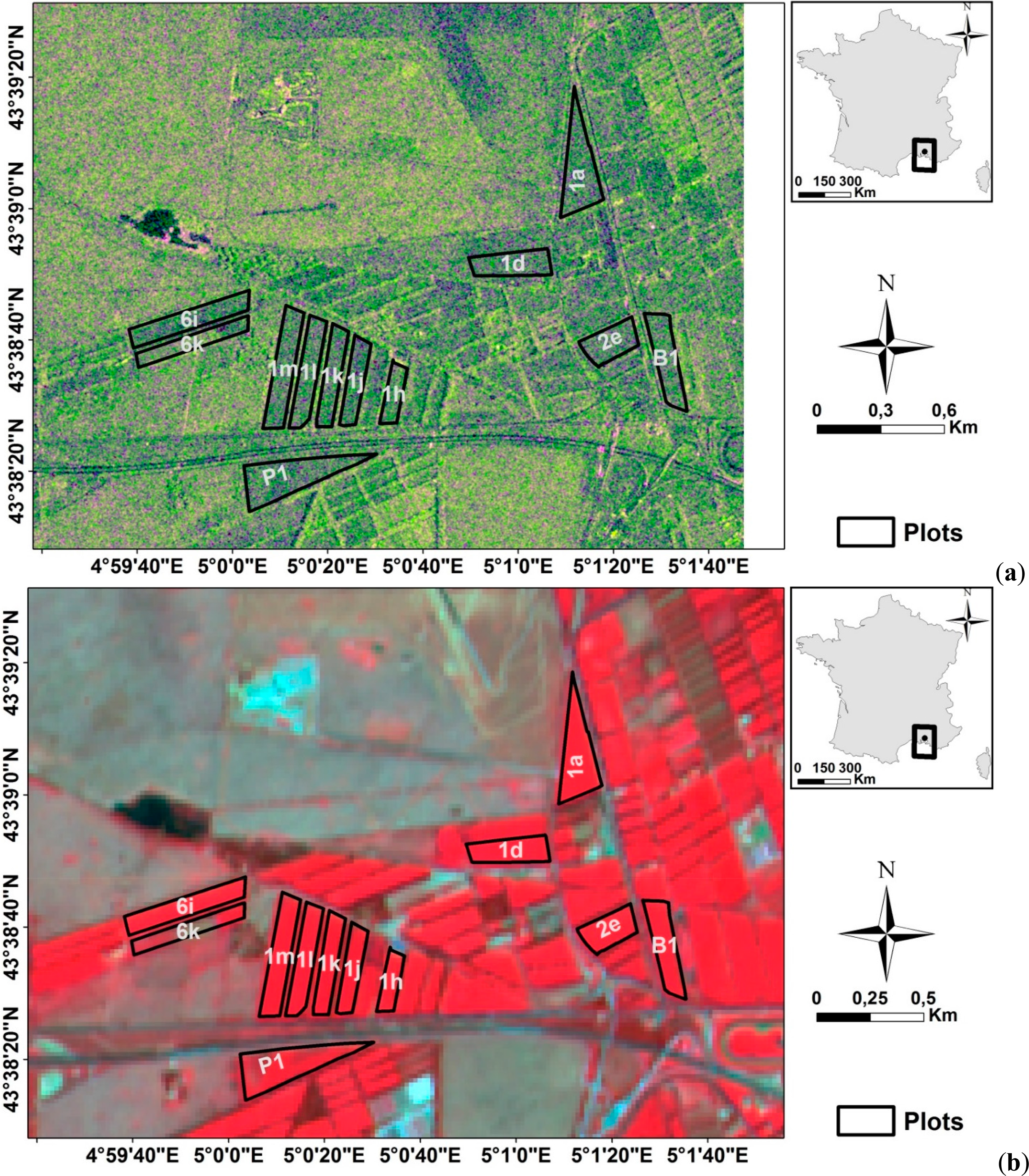
Our study site is the “Domaine du Merle”, an experimental farm of 450 hectares located in southeastern France (center: 43.64°N, 5.01°E, Figure 1). Within this farm, 150 hectares (52 parcels) are irrigated grasslands for hay production. The produced hay is certified (with the French label “AOP”) due to specific environmental factors and irrigation practices that ensure a high-quality floristic composition [69].
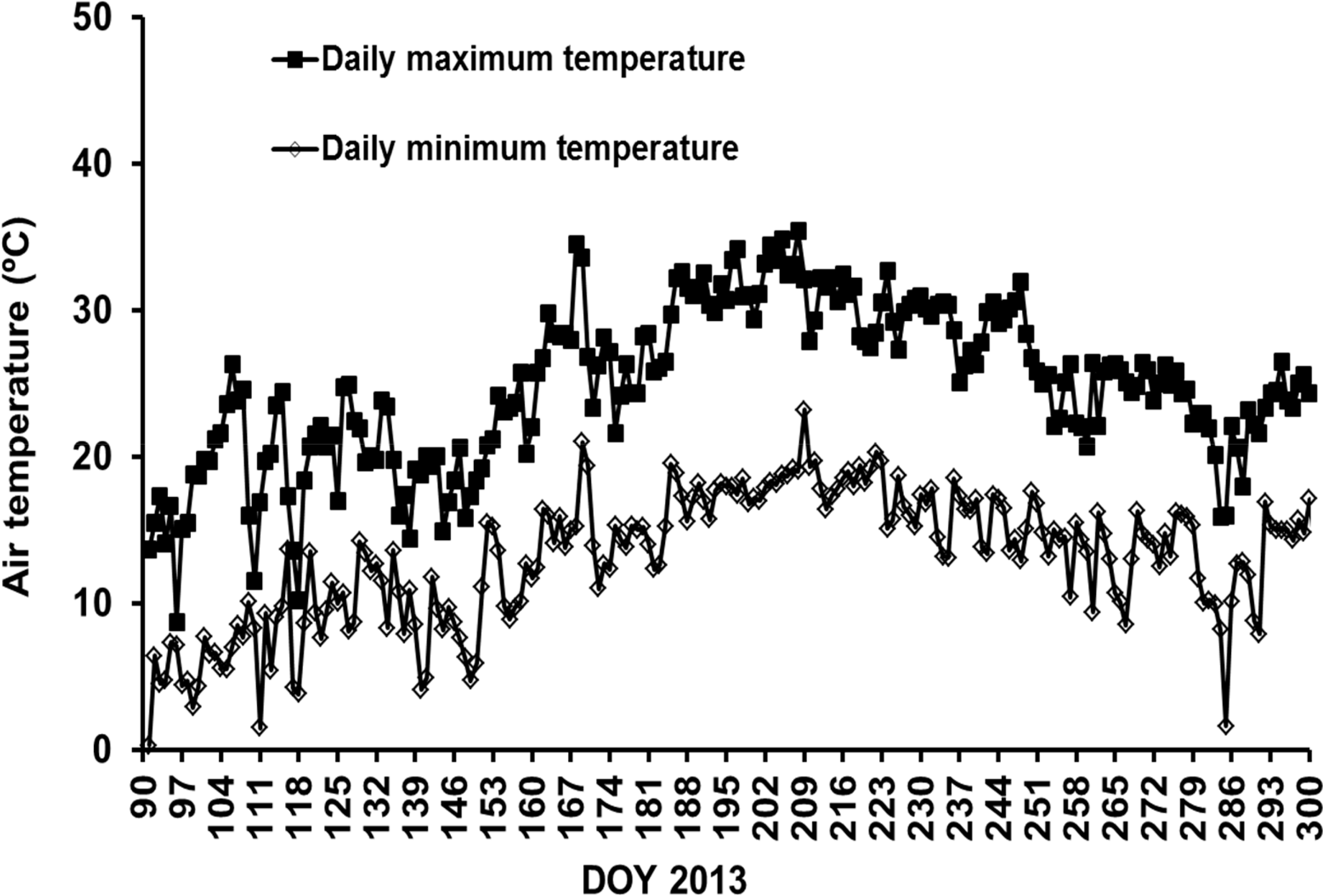
The study site is characterized by a Mediterranean climate, with a rainy season between September and November and an average cumulative rainfall between 350 mm and 800 mm [15]. The evaporation rate can reach 10 mm/day during the summer season due to high temperatures associated with dry and windy conditions. Hourly temperature and precipitation data acquired by a meteorological station installed at the study area were available. Figure 2 shows the mean daily air temperature recorded in 2013 during the remote sensing acquisitions (Tmean = 14.4 °C, and Tmax = 35.4 °C).
The soil has a mean retention capacity with concentrated vegetation roots in the upper 30 cm [70]. Moreover, the top soil is characterized by an absence or low presence of pebble (15%–20% of pebble stone at most) [69]. The top soil texture of the irrigated plots is a loam with a depth varying between 30 cm and 80 cm, depending on the plot age (between 10 years and three centuries) [69,71].
The plots were leveled with a very gentle slope that allows for surface irrigation by gravity (border irrigation). The total flow rate available for the farm (between 150 and 300 L/s) allows for the irrigation of one or two parcels simultaneously, the largest parcels being split into two or more subplots. Water is applied between March and September via canals, which bring water at the highest extremity of the subplots over a few hours. Water flows by gravity down to the lowest extremity of the plots. When the waterfront reaches 90% of the plot length, the water supply is stopped. The waterfront continues to flow and infiltrate until the tail end of the plot is reached. At the lowest side, excess water is evacuated through a drainage channel.
A rotation is applied so that all the parcels can be irrigated when necessary, approximately every 10 days on average. The plots are harvested three times a year, in May, June and September.
2.2. Satellite Data and in situ Measurements
2.2.1. SAR Images
Twenty-five X-band SAR images were acquired by COSMO-SkyMed (CSK) and TerraSAR-X (TSX) sensors between April and October 2013, with incidence angles between 28.3° and 32.5°; both the HH and HV polarizations were analyzed (Tables 1 and 2). The nine TSX images were acquired in “Stripmap mode”, with a ground pixel spacing of 3 m. Sixteen CSK images were obtained from the four satellites in the CSK constellation (six images from CSK1, four images from CSK2, one image from CSK3, and five images from CSK4) in “Stripmap Pingpong mode”, with a pixel size of 15 m.
Radiometric calibration of the SAR images was carried out using algorithms developed by the German Aerospace Center (DLR) and the Italian Space Agency (ASI). For TSX MGD (Multi Look Ground Range Detected) products, radiometric calibration was carried out using the following Equation (1):
This equation transforms the digital number of each pixel DN (the amplitude of the backscattered signal) into a backscattering coefficient (σ°) corrected for background sensor noise known as NESZ (Noise Equivalent Sigma Zero) on a linear scale. This calibration takes into account the radar incidence angle (θ) and the calibration constant (Ks) provided in the image data. The NESZ must be lower than the term Ks × DN2 × sin(θ) to ensure a high signal-to-noise ratio. For our TSX images, the NESZ varies from −25.2 dB to −22.6 dB for both HH and HV polarizations [1].
The calibration of the CSK images is given by the following formula:
The backscattering coefficients are then calculated in decibels using the following formula:
2.2.2. Optical Images
Thirty cloud-free optical images were also acquired by SPOT-4, SPOT-5, LANDSAT-7 and LANDSAT-8 sensors over the study area (Table 1). SPOT-4 images were acquired within the framework of the Take 5 experiment ( http://www.cesbio.ups-tlse.fr/). In most cases, the optical and radar images were not separated by more than four days.
Optical data processing includes orthorectification and correction for atmospheric effects. The atmospheric correction of SPOT-4 images was performed by CESBIO (Centre d’Etudes Spatiales de la BIOsphère) according to the method described by Hagolle et al. [73]. The atmospheric correction of SPOT-5 and LANDSAT-8 images was carried out using the simplified method of atmospheric correction (SMAC) [74]. Aerosol optical thickness at 550 nm and the water vapor content (g/m2), input variables in the SMAC model, were obtained from the AERONET (AErosol Robotic NETwork) website ( http://aeronet.gsfc.nasa.gov/). Finally, LANDSAT-7 surface reflectance images were downloaded directly from the USGS website ( http://earthexplorer.usgs.gov/). Atmospheric correction of LANDSAT-7 images was directly performed by the NASA (National Aeronautics and Space Administration) using specialized software called Landsat Ecosystem Disturbance Adaptive Processing System (LEDAPS). This software applies the 6S (Second Simulation of a Satellite Signal in the Solar Spectrum) radiative transfer model to produce surface reflectance data as described in [75]. The NDVI was computed from the optical images. Then, NDVI pixel values were averaged for each plot and compared to vegetation in situ measurements.
2.2.3. Experimental Measurements
In general, the in situ measurements were collected simultaneously with the SAR acquisitions to characterize the soil and vegetation variability (Table 1). Seven to ten training plots were sampled (see the locations in Figure 1). The dimension of sampled plot ranges between 2.13 ha and 7.23 ha.
Soil Measurements
Volumetric soil moisture measurements were conducted only in the first top 5 cm using calibrated TDR (Time Domain Reflectometry) probes; this was because the radar signal penetration depth in the soil surface is only a few centimetres at X-band [76]. Due to high evaporation rates, the soil moisture measurements were collected within a time window of 2 h around the satellite overpass time. Between 25 and 30 soil moisture measurements were performed for each training plot along regular transects. The volumetric soil moisture was then calculated for each training plot using the mean of all soil moisture measurements collected on the training plot, except for training plots where high spatial heterogeneity of the soil moisture was observed. This heterogeneity is frequent when the plot is under irrigation or when irrigation was finished a few hours before measurements were taken. In this case, several homogenous areas within the training plot were defined. The soil moisture content of each plot (or part of a plot) ranged from 0.10 cm3/cm3 to 0.47 cm3/cm3 (Table 2), with standard deviations between 0.01 and 0.05 cm3/cm3.
Measurements of soil roughness were carried out only once for each training plot using a needle profilometer 1 m in length with 2 cm sampling intervals. Ten roughness profiles were established in each training plot during the period where the vegetation was the lowest (in April). The following two surface roughness parameters were then calculated from these measurements: the average root mean square surface height (Hrms), which specifies the vertical scale of the roughness, and the correlation length (L), representing the horizontal scale [76]. The Hrms values varied between 0.35 and 0.55 cm. The correlation length (L) ranged from 2.00 to 4.60 cm. In general, the precision on the roughness measurements is influenced mainly by the length of the roughness profiles, the number of profiles, and the sampling interval of the profiles. It was demonstrated that significant errors are observed when short profiles with a low sampling interval are used [77,78]. For our smooth soils and X-band SAR data, roughness measurements with a sampling interval better than 1 cm would have been more precise. Given the homogeneous surface roughness in our study site, roughness parameters will not be considered in the sensitivity analysis of the X-band radar signal to soil moisture and vegetation parameters. However, these will be used in an upcoming work dedicated to model the radar signal according to soil and vegetation parameters.
Vegetation Measurements
Additional in situ measurements of vegetation were performed to estimate the following: the Leaf Area Index (LAI), the vegetation water content (VWC), biomass (BIO) and vegetation height (HVE). For each plot, 20–25 hemispherical digital photos were acquired at nadir using a fisheye lens. These photos were then processed using CAN-EYE imaging software to obtain the LAI ( http://www6.paca.inra.fr/can-eye). Moreover, two grass samples over a 50 cm × 50 cm square were collected to determine the fresh grassland biomass (wet weight per unit area). The fresh biomass was then driest to determine the vegetation water content (wet weight–dry weight). Finally, 20 vegetation height measurements were carried out for each training plot. All vegetation measurements within each plot were averaged to provide a mean value for each plot.
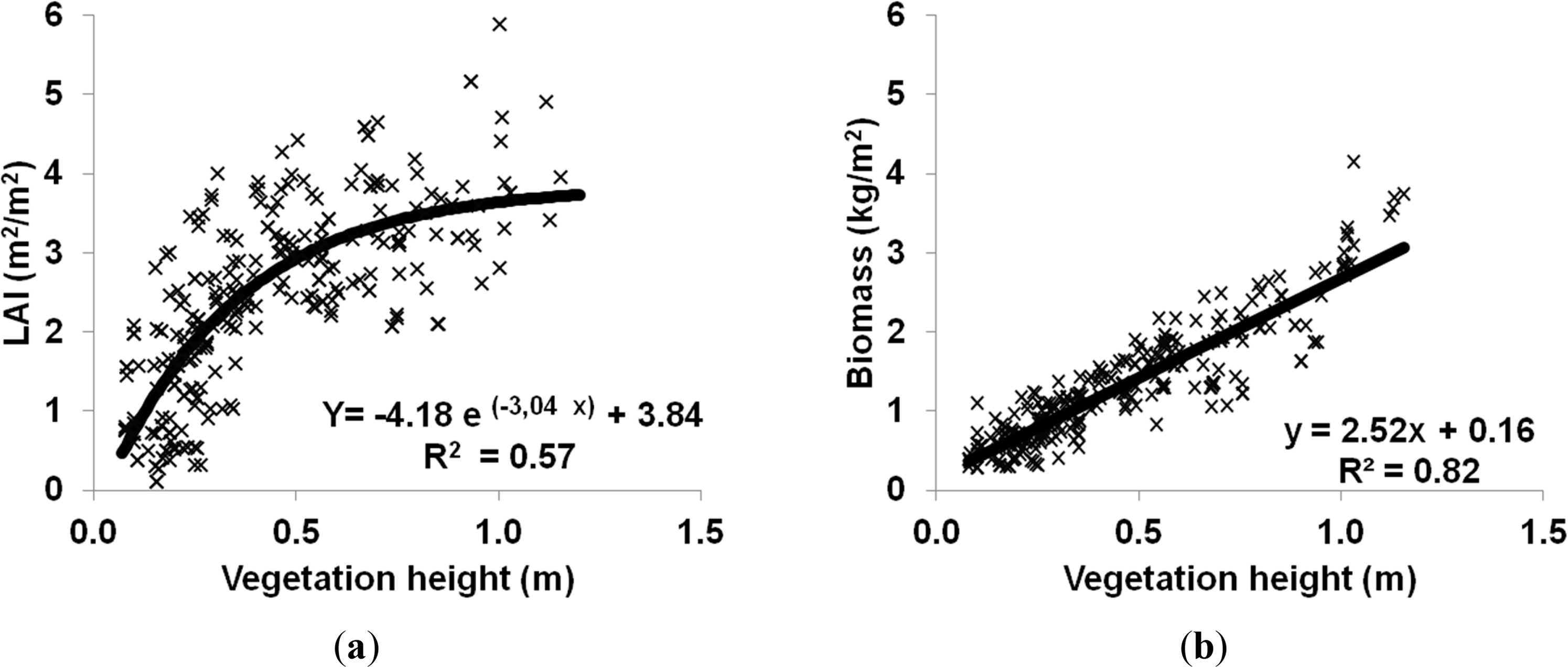
LAI measurements show a high variability due to very quick growth in the irrigated grasslands. For example, the LAI rises rapidly from 0.1 to 2 m2/m2 while the vegetation height increases from 10 to 50 cm (the biomass ranges between 0.3 and 1 kg/m2) (Figure 3a). A poor correlation (R2 = 0.49) is observed between the LAI and the grassland height when it is less than 50 cm. When the grassland height is greater than 50 cm, the LAI derived from optical photography tends to give saturated values (Figure 3a). The grassland biomass increases linearly with the vegetation height (Figure 3b).
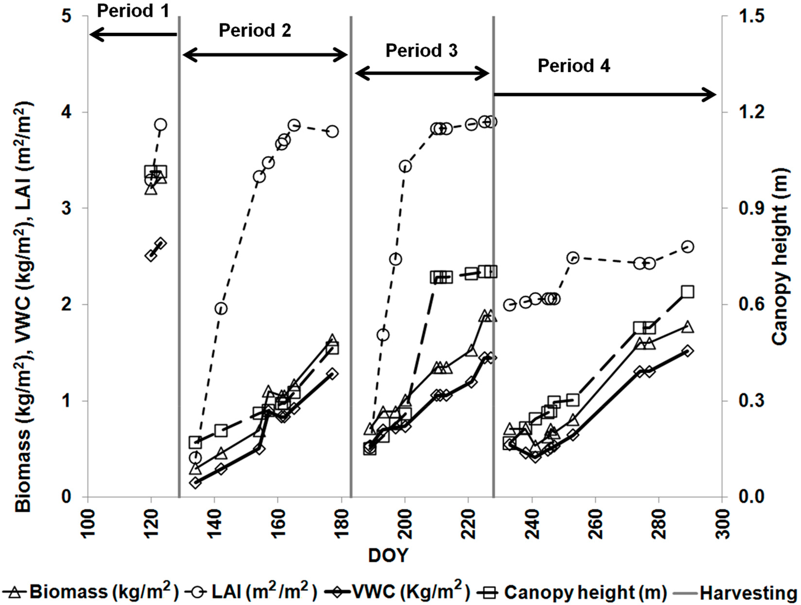
Figure 4 shows the temporal variations in the main vegetation parameters measured at the plot level. The three cuts of grassland are clearly identified on the graph in May (on approximately DOY 120) in June–July (on DOY 185) and in July–August (on DOY 230). Before the first cut, the vegetation parameters VWC, BIO and HVE are greater values in comparison to values measured during the other growth periods [69]. In general, the first yield always has greater hay production and is devoted to horses; the second and the third harvests are lower. The LAI usually reaches similar maximum values (approximately 3–4 m2/m2) during the first three growth periods (Figure 4). In the fourth period, the LAI values are lower (approximately 2–3 m2/m2). A strong correlation between the different vegetation parameters was observed (Figures 3 and 4). All vegetation parameters increase with time after harvesting, and this increase is very high during the first month of growth.
3. Results and Discussion
3.1. Relationships between NDVI and Vegetation Parameters
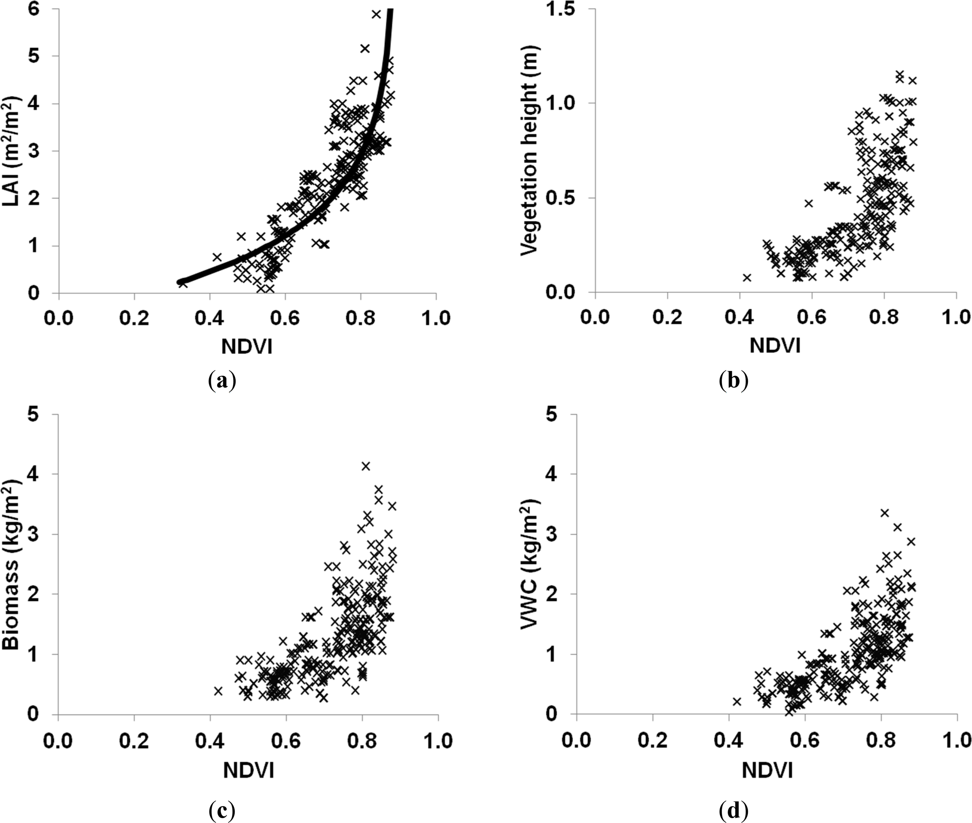
Figure 5a shows the relationship between the LAI estimated from ground measurements and the NDVI computed from different optical images. A classical logarithmic relationship is clearly observed, in accordance with similar results observed by Asrar et al. [5] and Bsaibes et al. [13], and is described by the following equation:
Courault et al. [15] found a kLAI of 0.71 from Formosat-2 images acquired on a larger area in the same region, including wheat, rice and irrigated grassland. For wheat plots on the Kairouan plain (Tunisia), Zribi et al. [46] found a kLAI of 1.24.
The correlations between the NDVI and the vegetation parameters HVE, BIO and VWC are displayed in Figure 5b–d. For these graphs, a linear relationship is observed between NDVI and the vegetation variables when the NDVI is less than 0.8. Above this, the NDVI saturates and does not vary with increases in the different vegetation parameters (the threshold value for the estimation of HVE from the NDVI is 30 cm, and the threshold is approximately 1 kg/m2 for BIO and VWC).
3.2. The Radar Response According to Soil Moisture Variations
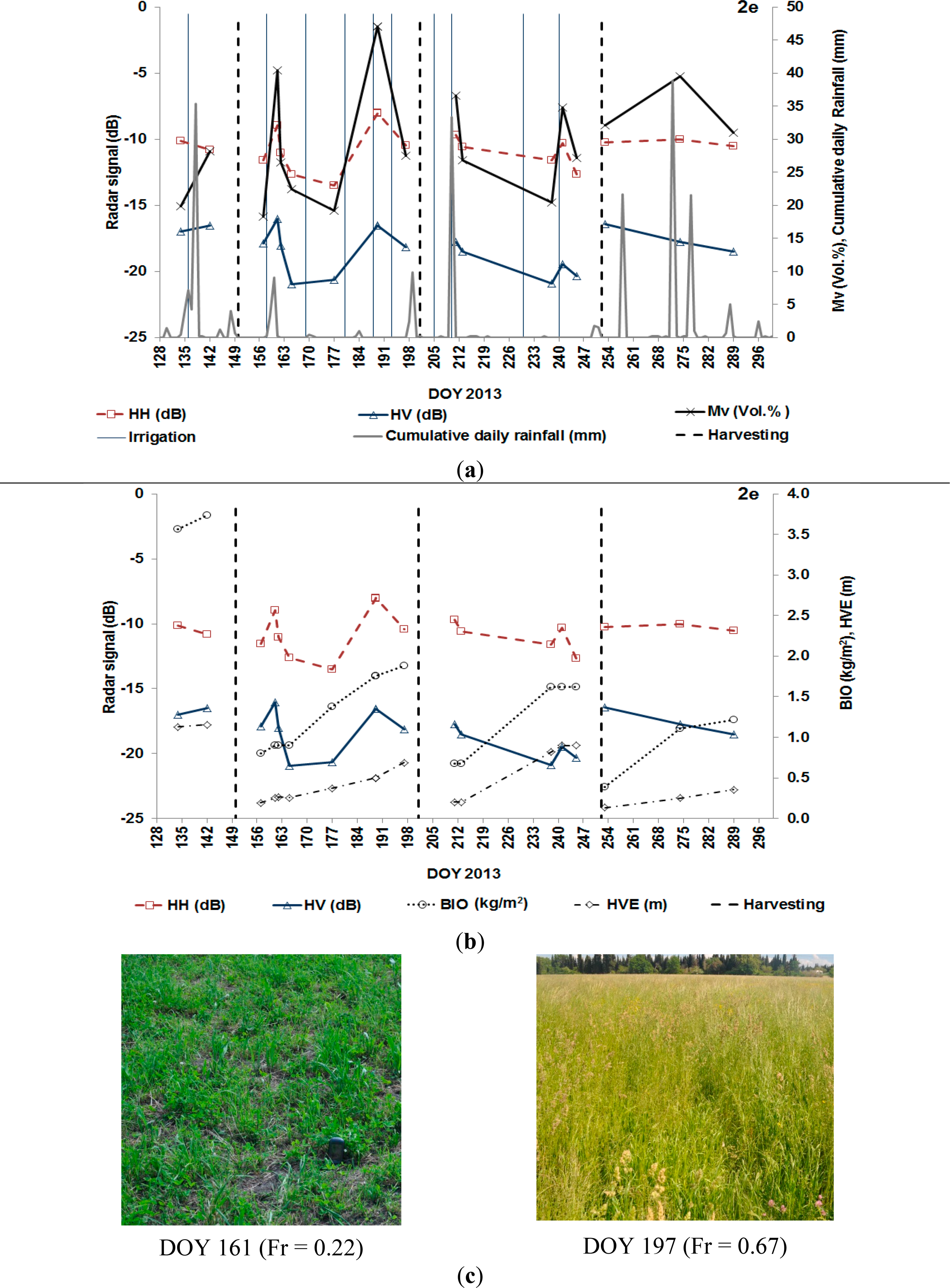
Figure 6 shows the temporal variations in the radar signal for HH and HV polarizations according to the soil moisture measurements (plot 2e). It shows that the behavior of the radar signal follows the evolution of soil moisture throughout the entire vegetation stage. Similar results were observed for all sampled plots.
The first cut occurred in early June (on DOY 150), and the first irrigation that followed was on DOY 158. Before the first irrigation, the soil moisture was approximately 0.18 cm3/cm3 (on DOY 157). After the first irrigation (on DOY 158) two rainfall events occurred (on DOY 159 and DOY 160, with 3.2 and 9.2 mm precipitation, respectively). Following these events, the soil moisture considerably increased (to approximately 0.40 cm3/cm3 on DOY 161). As a result, the radar signal increased between DOY 157 and DOY 161 in both the HH and HV polarizations of approximately 2.6 dB and 1.9 dB, respectively (the Mv increased to approximately 0.22 cm3/cm3; the HVE was approximately 25 cm). On the SAR image acquired on DOY 162 (4 days after irrigation), HH and HV decreased approximately 2.1 dB due to a decrease in moisture from 0.40 to 0.26 cm3/cm3. On the SAR image acquired on DOY 165, the radar signal continued to decrease due to a decrease in soil moisture (approximately 0.22 cm3/cm3).
Following irrigation on DOY 189, the in situ soil moisture was approximately 0.47 cm3/cm3 on DOY 189; the radar signal was high (σ°HH = −8.0 dB and σ°HV = −16.5 dB) and the HVE was approximately 47 cm. Following a large rainfall on DOY 210 (33 mm) and irrigation on DOY 211, the radar signal on DOY 211 showed high HH and HV values (σ°HH = −9.7 dB and σ°HV = −17.7 dB). After two days (on DOY 213), the soil moisture decreased from 0.37 to 0.27 cm3/cm3; the associated radar signal also decreased.
On DOY 241, one day after irrigation on DOY 240, the soil contribution was high on the total backscattered signal despite a HVE high value (HVE approximately 90 cm). Indeed, the radar signal increased approximately 1.4 dB in both HH and HV between DOY 238 and DOY 241 (the Mv increased from 0.20 to 0.35 cm3/cm3).
In conclusion, the results show that the radar signal could be used to identify three-day-old irrigated plots.
3.3. Sensitivity of Radar Signal to Soil Moisture
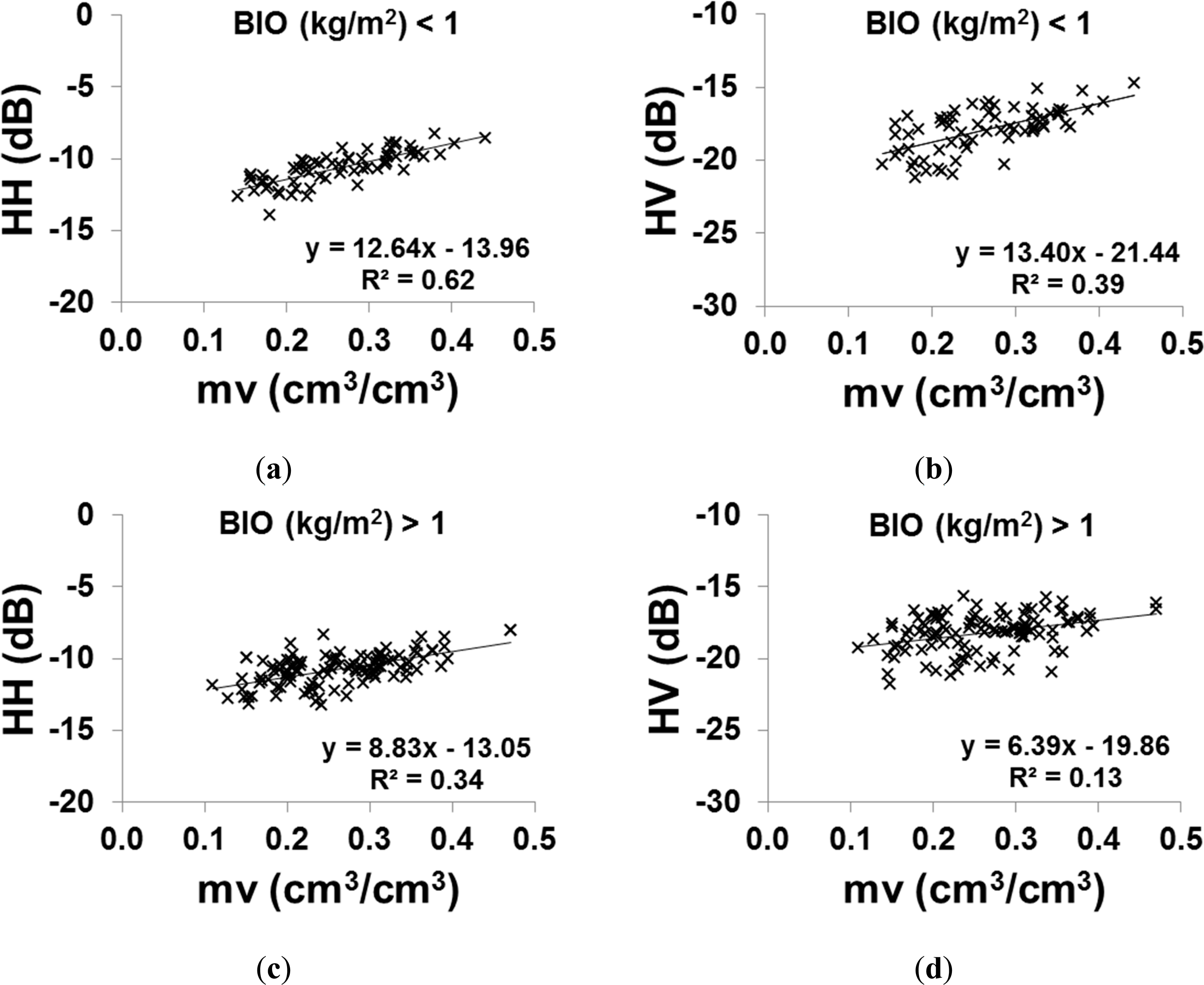
The sensitivity of X-band SAR signal to soil moisture was studied for two biomass classes: BIO < 1 kg/m2 and BIO > 1 kg/m2. The BIO = 1 kg/m2 limit corresponds to a vegetation height of approximately 30 cm, a vegetation water content of 0.8 kg/m2, and a LAI of approximately 2 m2/m2. First, the mean backscattering coefficients were calculated from calibrated TSX and CSK images over all sampled plots by averaging the linear σ° values of all pixels within the non-flooded training plots or within the non-flooded portions of irrigated plots.
Figure 7 shows that the radar signal for HH and HV polarizations is clearly dependent on soil moisture, with sensitivity to soil moisture for BIO lower than 1 kg/m2 of approximately 12.64 and 13.40 dB/[cm3/cm3] at HH and HV, respectively. Baghdadi et al. [79] showed that when TerraSAR-X data are used after strong rains, the soil contribution (influenced by soil moisture) to the backscattering of sugarcane plots is important when the cane height is less than 30 cm. For BIO higher than 1 kg/m2, the sensitivity of the radar signal to soil moisture decreases to 8.83 and 6.39 dB/[cm3/cm3] at HH and HV, respectively. These results demonstrated that the soil contribution to the X-band SAR signal could be high for grassland biomass lower than 1 kg/m2 in both the HH and HV polarizations; the soil contribution also decreases more quickly in HV than in HH for BIO higher than 1 kg/m2. These results show that the SAR X-band signal, mainly in HH polarization, can penetrate the canopy and interact with the soil even for vegetation with biomass (when BIO>1 kg/m2). When biomass is both lower and higher than 1 kg/m2, the radar response showed more variability for the same soil moisture range in HV than in HH; this is due to the sensitivity of HV polarization to vegetation cover, which has already been observed by Balenzano et al. [80], Brown et al. [81], and Picard et al. [82].
In conclusion, these results show that the X-band radar signal at a medium incidence angle (30°) depends on the soil moisture, regardless of the vegetation conditions. This dependence could be improved with SAR data at lower incidence angles. Indeed, the penetration depth of the radar signal into the vegetation cover is higher at low incidence angles.
3.4. Detection of Flooded Plots
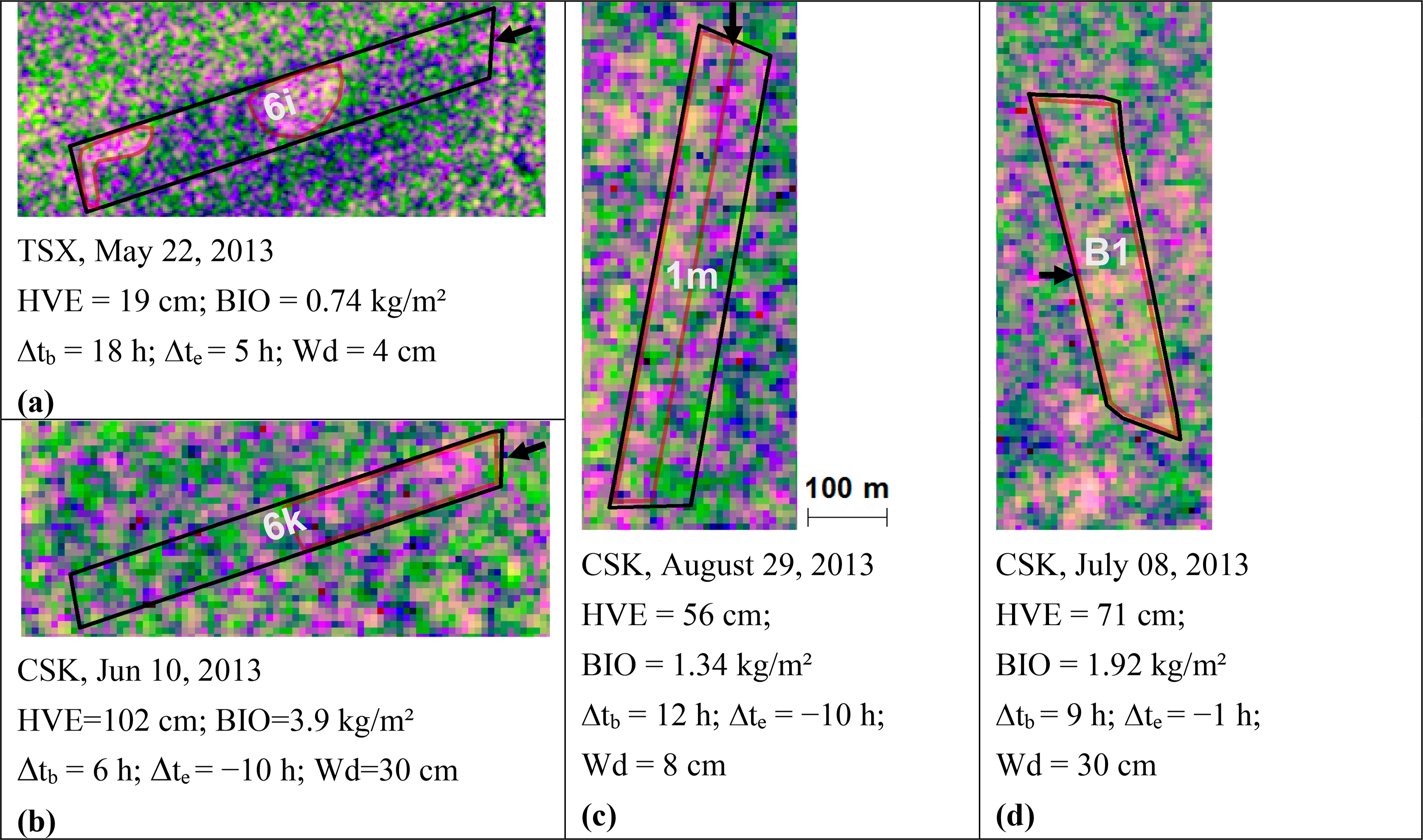
Thanks to the high spatial resolution of the selected radar images (3 m × 3 m for TSX, and 8 m × 8 m for CSK), photo interpretation makes it possible to detect which parts of the plots are flooded by gravity irrigation. The “Domaine du Merle” grassland plots are irrigated every 10 days on average, for between 10 and 30 h. The interpretation of SAR X-band images shows that the X-band allows for the tracking of irrigation practices. An analysis of the radar signal was conducted on plots under irrigation at the time of the SAR acquisitions (Figure 8b–d) and on plots where irrigation was completed a few hours earlier (Figure 8a) In situ observations showed that water bodies present on irrigated plots in some locations varied from a few centimeters to thirty centimeters. In plot 6i, in situ observations showed that the plot was entirely irrigated during the SAR overpass (the SAR image was acquired 5 h after irrigation) with the presence of two water bodies (Figure 8a). The presence of water could be explained by a leveling defect in some areas and low hydraulic conductivity preventing the quick infiltration of water.
The analysis showed a higher radar signal at locations with water bodies than at locations without water bodies. The brightest radar returns were caused by double-bounce scattering between the water surface and the vertical stems and leaves of the vegetation. The difference in the radar signal level (∆) between the flooded areas and the unflooded areas is generally two times greater in HH compared to HV (∆HH∼5.5 dB and ∆HV∼3.5 dB). This is due to the attenuation of the backscattered radar signal by the vegetation, which is more significant at HV polarization than at HH polarization. Baghdadi et al. [83] found also that the potential of HH polarization is higher than HV and VV polarizations in a study mapping wetlands from C-band SAR data. Our results also showed that the penetration depth of the radar wave in the X-band is high, even for dense and tall vegetation. For HVE between 20 and 55 cm and water bodies with depths between 4 and 10 cm, flooded areas are clearly visible on the images (Figure 8a,c). A strong penetration was also observed in other training grassland plots with HVE between 71 and 102 cm and water bodies with depths of approximately 30 cm (Figure 8b,d). These plots corresponded to wet biomass (BIO) values up to 3.9 kg/m2.
3.5. Relationships between Radar Signals and Vegetation Parameters
In this section, the backscattered signal was analyzed as a function of vegetation parameters (LAI, HVE, BIO, and VWC). Grassland plots contain approximately 20 different species of vegetation. The main vegetation species are grasses (Dactylis glomerata L., Lolium perenne L., Poa pratensis L., Holcus lanatus L., Arrhenatherum elatius L., Festuca pratensis L., Setaria glaucus L., and Paspalum dilatatum Poir), legumes (Medicago lupulina L., Trifolium repens L., Trifolium pretense L., Lotus corniculatus L., and Viccia cracca L.), and diverse dicotyledons (Plantago lanceolata L., Taraxacum officinaleWeber., Tragopogon pratensis L., Galium mollugo L., Galium verum L., Daucus carota L., Achellea millefolium L., Pastanica silvestris L., and Rumex acetosa L.) [84]. At plot scale, the vegetation structure geometry is homogeneous. The biomass levels of these species vary during the growth season. In the first growth period, grass species are dominant (60%–65%). Grass biomass levels decrease in the second and third growth periods. However, legume and diverse dicotyledon biomass levels increase from 35%–40% in the first period to 55% in the third period [69]. An important change in morphology is observed, especially in grass species, when vegetation exceeds approximately 50 cm (LAI about 2 m2/m2, BIO about 1.5 kg/m2 and VWC about 1.2 kg/m2); inclined elements (panicle, small leave, etc.) randomly oriented at the top of the plant begin to appear. The VWC and plant morphology are the main vegetation variables that affect the radar response [85]. It was therefore essential to study the relationship between the radar signal and vegetation parameters (LAI, HVE, BIO and VWC) separately according to two vegetation classes (LAI, HVE, BIO and VWC lower and higher than 2 m2/m2, 50 cm, 1.5 kg/m2, and 1.2 kg/m2, respectively). To reduce the effect of soil moisture on the analysis of the backscattered radar signal, relationships between radar signals and vegetation parameters were traced according to three classes of soil moisture (Mv < 0.2, 0.2 < Mv < 0.3 and Mv > 0.3 cm3/cm3).
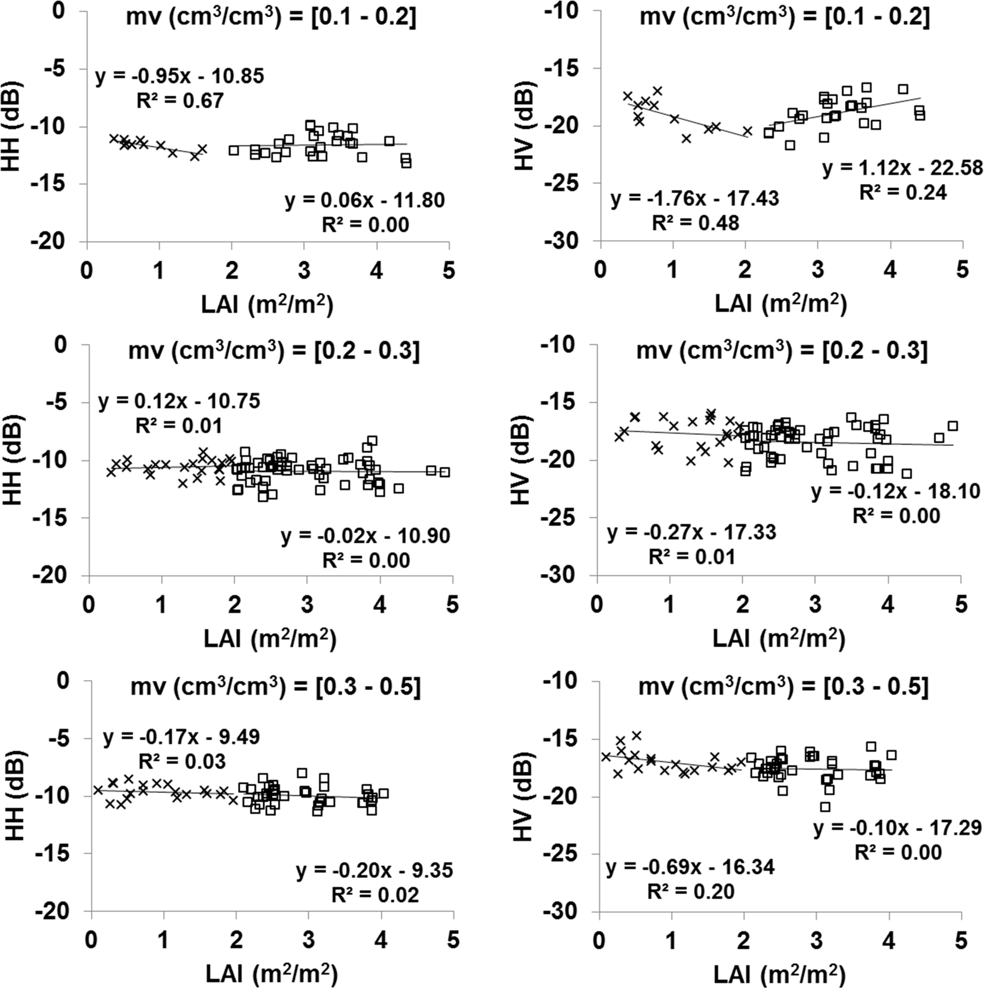
Figure 9 shows the behavior of the SAR X-band signal according to LAI. The results showed that for soil moisture between 0.10 and 0.20 cm3/cm3, the radar signal in HH and HV decreases with LAI for LAI lower than 2 m2/m2, and increases as the LAI increases from 2 m2/m2 to 5 m2/m2. These variations in the radar signal (decrease and increase) are higher in HV polarization than in HH polarization (Figure 9 first row). The decrease in radar signal for LAI lower than 2 m2/m2 is related to an increase in the attenuation of the soil contribution; this is more important than the enhanced contribution from the vegetation canopy [80,81,86]. In addition, the increase in the vegetation contribution as a function of the LAI, combined with the decrease in the soil moisture contribution (Mv between 0.10 and 0.20 cm3/cm3), results in a slight increase in the radar backscatter with LAI for values greater than 2 m2/m2. For Mv between 0.20 and 0.50 cm3/cm3, the radar signal slightly decreases in HH and HV polarization for LAI between about 0.1 and 5.0 m2/m2 (Figure 9 second row and third row). Indeed, for Mv between 0.20 and 0.50 cm3/cm3, the decrease of the soil contribution when LAI increases between 0.1 and 5.0 m2/m2 is of the same order than the increase of the vegetation contribution. Many studies have analyzed the behavior of radar signals (Ku, X, C and L bands) as a function of LAI [87–93]. Previous results have shown that the radar signal decreases with an increase in the LAI for narrow leaf crops (wheat, alfalfa, and barley), and increases for board leaf crops (sunflower, corn, sorghum, and sugarcane) [91,93]. For example, Champion [87] studied the sensitivity of radar signals in C and X bands to the LAI of wheat crops (soil moisture values between 0.05 and 0.20 cm3/cm3) in using HH and VV polarizations (20° for the C band and 40° for the X band). In this study, the signal decreased approximately 8 dB in the X-band for LAI values between 0.1 and 3 m2/m2, and the signal decreased approximately 12 dB in the C-band for LAI between 0.1 and 4 m2/m2. The signals at C and X bands increase approximately 7 dB with LAI for LAI values up to 8 m2/m2. Similar results on the behavior of X-VV radar signal according to LAI of wheat were found by Prevot et al. [59] for soil moisture values between 0.05 cm3/cm3 and 0.20 cm3/cm3. Fieuzal et al. [88] analyzed wheat crops with LAI values between 1 and 4 m2/m2 in wet soil conditions (soil moistures between 0.20 and 0.40 cm3/cm3); the radar signals in the X and C bands decreased with the LAI by approximately −2.6 dB by 1 m2/m2 for X-HH and −2.4 dB by 1 m2/m2 for C-VV. The C-HH and C-HV signals have lower sensitivity, with about −1 dB by 1 m2/m2. Ulaby et al. [92] demonstrated that the radar signal at Ku-VV (50°) increases with the LAI of corn and sorghum, up to LAI of approximately 2 m2/m2; beyond this, the radar signal saturates. Lin et al. [89] observed increasing radar responses in sugarcane plots when the sugarcane LAI increased (with the C-band and incidence between 31° and 39°). This increase is greater in HV than in HH due to higher volume scattering in HV compared to HH. In a study by Liu et al. [90], the radar signal in the C band (24° and 47°) increased with the LAI in soybean and corn crops.
Figure 10 shows the behavior of the SAR X-band signal according to HVE using different soil moisture classes. The results showed that for vegetation heights lower than 50 cm, the radar signal decreases with HVE. This decrease in the radar signal for vegetation heights lower than 50 cm is higher in HV polarization than in HH polarization (approximately −0.5 dB and −1.1 dB by 10 cm in HH and HV, respectively). The attenuation is stronger for HV than for HH due to the vertical plant stems, and the attenuation increases with stem height [81,82,86,94]. Consequently, the soil contribution to the total backscatter is lower at HV than at HH polarization. Fieuzal et al. [88] showed that for wheat height is between approximately 3 cm and 65 cm, the radar signal at X-HH decreases by 1.3 dB as the HVE of wheat increases by 10 cm. Beyond 50 cm, the radar signal slightly increases at both HH and HV when head element flowers begin to appear at the top layer of grassland vegetation (Figure 9). When plants are higher than 50 cm, the backscattered signal is mainly due to the leaves, stems and the head element flowers [94]. According to Figures 6 and 7, the soil also contributes slightly to HVE higher than 50 cm. The increase in the radar signal from HVE above 50 cm is greater in HV than in HH due to the greater contribution of vegetation in HV than in HH.
Figures 11 and 12 show the behavior of the SAR X-band signal according to BIO and VWC using different soil moisture classes. Result shows that the HH polarization appears to be insensitive to fresh biomass and vegetation water content. The results also showed that HV slightly decreases with BIO and VWC (BIO and VWC are well correlated) to a threshold about 1.5 kg/m2, then increases slightly.
Overall, the use of X-band radar signal with medium incidence angle (∼30°) for the retrieval of LAI, HVE, BIO, and VWC of our grassland is very limited. Only the canopy height could be retrieved for heights lower than 50 cm and in using HV polarization. Results show that the opportunity to estimate the soil moisture even with dense vegetation covers (vegetation height up to 1 m). Indeed, the X-band radar signal penetrates vegetation cover and always follows the evolution of soil moisture. In the future, the opportunity to estimate soil water content using semi-empirical backscattering models (such as water cloud model) will be investigated.
4. Conclusions and Perspectives
This study analyzed the temporal signature of SAR X-band signals acquired over irrigated grassland plots over several growing cycles. The objective of this work was to investigate the sensitivity of radar signals to soil moisture and vegetation parameters (LAI, vegetation height, biomass, and vegetation water content).
Our results show that the radar signal in the X-band at both HH and HV polarizations is always sensitive to soil moisture variations, even with dense vegetation cover (HVE up to 1 m). This sensitivity decreases as vegetation density increases (higher sensitivity for biomass lower than 1 kg/m2). This result proves that the X-band radar signal penetrates the grassland cover (with vegetation height up to 1 m) and allows for the tracking of irrigation practices. In addition, the X-band at HV polarization is more sensitive to grassland parameters than at HH polarization; however, the potential use of the X-band for the monitoring of vegetation parameters is very limited. The X-band radar signal at HV polarization is useful for the monitoring of HVE up to 50 cm.
The X-band radar signal is sensitive enough to variations in soil moisture to monitor soil moisture over grasslands. An inversion method based on backscattering models should be developed to analyze the precision of soil moisture estimates using X-band radar images over grassland. The objective of our future work is to develop methodologies based on the coupling of X-band SAR and optical data to estimate soil moisture. The arrival of Sentinel-1 and Sentinel-2 constellations, which have the ability to provide images with high repetition, will allow scientists to combine optical and radar images to estimate soil moisture in agricultural environments.
Acknowledgments
This research was supported by the French Space Study Center (CNES, DAR 2013 TOSCA) and the Islamic development bank (PhD Scholarship of M. Mohammad El Hajj). Field experiments were carried out within the SicMed-Crau program. The CSK images used in this analysis were supported by public funds received in the GEOSUD framework, a project (ANR-10-EQPX-20) of the “Investissements d’Avenir” program managed by the French National Research Agency. The authors wish to thank the German Space Agency (DLR) for kindly providing the TSX images under proposal HYD0007. We also wish to thank the EMMAH unit (INRA) for providing meteorological data and the technical teams of ASI and DLR for providing answers regarding the performances of CSK and TSX. Finally, we would like to thank the CNES-CESBIO (Centre d'Etudes Spatiales de la BIOsphère) for providing calibrated SPOT-4 images in the framework of Take 5 experiments.
Author Contributions
EL Hajj M. and Baghdadi N. conceived and designed the experiments; EL Hajj M. performed the experiments; EL Hajj M. and Baghdadi N. analyzed the data; Belaud G., Zribi M., Cheviron B., Courault D., Hagolle O., and Charron F. revised the manuscript; EL-Hajj wrote the article.
Conflicts of Interest
The authors declare no conflict of interest.
References
- Eineder, M.; Fritz, T.; Mittermayer, J.; Roth, A.; Boerner, E.; Breit, H. TerraSAR-X Ground Segment, Basic Product Specification Document; DTIC Document; Cluster Applied Remote Sensing: Munich, Germany, 2008. [Google Scholar]
- Schwerdt, M.; Bräutigam, B.; Bachmann, M.; Döring, B. TerraSAR-X calibration results. Proceedings of the 2008 7th European Conference on Synthetic Aperture Radar (EUSAR), Friedrichshafen, Germany, 2–5 June 2008; pp. 1–4.
- Agenzia Spaziale Italiana. COSMO-SkyMed System Description & User Guide; Agenzia Spaziale Italiana: Roma, Italy, 2007. Available online: http://www.cosmo-skymed.it/docs/ASI-CSM-ENGRS-093-A-CSKSysDescriptionAndUserGuide.pdf (accessed on 15 October 2014).
- Iorio, M.; Mecozzi, R.; Torre, A. Cosmo SkyMed: Antenna elevation pattern data evaluation. Ital. J. Remote Sens 2010, 42, 69–77. [Google Scholar]
- Asrar, G.; Fuchs, M.; Kanemasu, E.T.; Hatfield, J.L. Estimating absorbed photosynthetic radiation and leaf area index from spectral reflectance in wheat. Agron. J 1984, 76, 300–306. [Google Scholar]
- Baret, F.; Guyot, G. Potentials and limits of vegetation indices for LAI and APAR assessment. Remote Sens. Environ 1991, 35, 161–173. [Google Scholar]
- Baret, F.; Hagolle, O.; Geiger, B.; Bicheron, P.; Miras, B.; Huc, M.; Berthelot, B.; Niño, F.; Weiss, M.; Samain, O. LAI, fAPAR and fCover CYCLOPES global products derived from VEGETATION: Part 1: Principles of the algorithm. Remote Sens. Environ 2007, 110, 275–286. [Google Scholar]
- Carlson, T.N.; Ripley, D.A. On the relation between NDVI, fractional vegetation cover, and leaf area index. Remote Sens. Environ 1997, 62, 241–252. [Google Scholar]
- Duchemin, B.; Hadria, R.; Erraki, S.; Boulet, G.; Maisongrande, P.; Chehbouni, A.; Escadafal, R.; Ezzahar, J.; Hoedjes, J.C.B.; Kharrou, M.H. Monitoring wheat phenology and irrigation in Central Morocco: On the use of relationships between evapotranspiration, crops coefficients, leaf area index and remotely-sensed vegetation indices. Agric. Water Manag 2006, 79, 1–27. [Google Scholar]
- Weiss, M.; Baret, F. Evaluation of canopy biophysical variable retrieval performances from the accumulation of large swath satellite data. Remote Sens. Environ 1999, 70, 293–306. [Google Scholar]
- Weiss, M.; Baret, F.; Smith, G.J.; Jonckheere, I.; Coppin, P. Review of methods for in situ leaf area index (LAI) determination: Part II. Estimation of LAI, errors and sampling. Agric. For. Meteorol 2004, 121, 37–53. [Google Scholar]
- Baret, F.; Guerif, M. Remote detection and quantification of plant stress: Opportunities remote sensing observations. Comp. Biochem. Physiol. Mol. Integr. Physiol 2006, 143, S148–S148. [Google Scholar]
- Bsaibes, A.; Courault, D.; Baret, F.; Weiss, M.; Olioso, A.; Jacob, F.; Hagolle, O.; Marloie, O.; Bertrand, N.; Desfond, V. Albedo and LAI estimates from FORMOSAT-2 data for crop monitoring. Remote Sens. Environ 2009, 113, 716–729. [Google Scholar]
- Courault, D.; Bsaibes, A.; Kpemlie, E.; Hadria, R.; Hagolle, O.; Marloie, O.; Hanocq, J.-F.; Olioso, A.; Bertrand, N.; Desfonds, V. Assessing the potentialities of FORMOSAT-2 data for water and crop monitoring at small regional scale in South-Eastern France. Sensors 2008, 8, 3460–3481. [Google Scholar]
- Courault, D.; Hadria, R.; Ruget, F.; Olioso, A.; Duchemin, B.; Hagolle, O.; Dedieu, G. Combined use of FORMOSAT-2 images with a crop model for biomass and water monitoring of permanent grassland in Mediterranean region. Hydrol. Earth Syst. Sci. Discuss 2010, 7, 1731–1744. [Google Scholar]
- Edirisinghe, A.; Hill, M.J.; Donald, G.E.; Hyder, M. Quantitative mapping of pasture biomass using satellite imagery. Int. J. Remote Sens 2011, 32, 2699–2724. [Google Scholar]
- Ferreira, L.G.; Fernandez, L.E.; Sano, E.E.; Field, C.; Sousa, S.B.; Arantes, A.E.; Araújo, F.M. Biophysical properties of cultivated pastures in the Brazilian savanna biome: An analysis in the spatial-temporal domains based on ground and satellite data. Remote Sens 2013, 5, 307–326. [Google Scholar]
- Schino, G.; Borfecchia, F.; de Cecco, L.; Dibari, C.; Iannetta, M.; Martini, S.; Pedrotti, F. Satellite estimate of grass biomass in a mountainous range in central Italy. Agrofor. Syst 2003, 59, 157–162. [Google Scholar]
- Todd, S.W.; Hoffer, R.M.; Milchunas, D.G. Biomass estimation on grazed and ungrazed rangelands using spectral indices. Int. J. Remote Sens 1998, 19, 427–438. [Google Scholar]
- Payero, J.O.; Neale, C.M.U.; Wright, J.L. Comparison of eleven vegetation indices for estimating plant height of alfalfa and grass. Appl. Eng. Agric 2004, 20, 385–393. [Google Scholar]
- Chen, D.; Huang, J.; Jackson, T.J. Vegetation water content estimation for corn and soybeans using spectral indices derived from MODIS near-and short-wave infrared bands. Remote Sens. Environ 2005, 98, 225–236. [Google Scholar]
- Jackson, T.J.; Chen, D.; Cosh, M.; Li, F.; Anderson, M.; Walthall, C.; Doriaswamy, P.; Hunt, E. Vegetation water content mapping using Landsat data derived normalized difference water index for corn and soybeans. Remote Sens. Environ 2004, 92, 475–482. [Google Scholar]
- Serrano, L.; Ustin, S.L.; Roberts, D.A.; Gamon, J.A.; Penuelas, J. Deriving water content of chaparral vegetation from AVIRIS data. Remote Sens. Environ 2000, 74, 570–581. [Google Scholar]
- Gu, Y.; Brown, J.F.; Verdin, J.P.; Wardlow, B. A five - year analysis of MODIS NDVI and NDWI for grassland drought assessment over the central Great Plains of the United States. Geophys. Res. Lett 2007, 34. [Google Scholar] [CrossRef]
- Gao, B.-C. NDWI—A normalized difference water index for remote sensing of vegetation liquid water from space. Remote Sens. Environ 1996, 58, 257–266. [Google Scholar]
- Anderson, M.C.; Neale, C.M.U.; Li, F.; Norman, J.M.; Kustas, W.P.; Jayanthi, H.; Chavez, J. Upscaling ground observations of vegetation water content, canopy height, and leaf area index during SMEX02 using aircraft and Landsat imagery. Remote Sens. Environ 2004, 92, 447–464. [Google Scholar]
- Aubert, M.; Baghdadi, N.; Zribi, M.; Douaoui, A.; Loumagne, C.; Baup, F.; El Hajj, M.; Garrigues, S. Analysis of TerraSAR-X data sensitivity to bare soil moisture, roughness, composition and soil crust. Remote Sens. Environ 2011, 115, 1801–1810. [Google Scholar]
- Baghdadi, N.; Gaultier, S.; King, C. Retrieving surface roughness and soil moisture from SAR data using neural networks. In Retrieval of Bio-and Geo-Physical Parameters from SAR Data for Land Applications; ESTEC Publishing Division: Sheffield UK, 2002; Volume 475, pp. 315–319. [Google Scholar]
- Baghdadi, N.; Cresson, R.; El Hajj, M.; Ludwig, R.; la Jeunesse, I. Estimation of soil parameters over bare agriculture areas from C-band polarimetric SAR data using neural networks. Hydrol. Earth Syst. Sci 2012, 16, 1607–1621. [Google Scholar]
- Srivastava, H.S.; Patel, P.; Sharma, Y.; Navalgund, R.R. Large-area soil moisture estimation using multi-incidence-angle RADARSAT-1 SAR data. IEEE Trans. Geosci. Remote Sens 2009, 47, 2528–2535. [Google Scholar]
- Zribi, M.; Saux-Picart, S.; André, C.; Descroix, L.; Ottle, C.; Kallel, A. Soil moisture mapping based on ASAR/ENVISAT radar data over a Sahelian region. Int. J. Remote Sens 2007, 28, 3547–3565. [Google Scholar]
- Zribi, M.; Baghdadi, N.; Holah, N.; Fafin, O. New methodology for soil surface moisture estimation and its application to ENVISAT-ASAR multi-incidence data inversion. Remote Sens. Environ 2005, 96, 485–496. [Google Scholar]
- Zribi, M.; Dechambre, M. A new empirical model to retrieve soil moisture and roughness from C-band radar data. Remote Sens. Environ 2003, 84, 42–52. [Google Scholar]
- Inoue, Y.; Kurosu, T.; Maeno, H.; Uratsuka, S.; Kozu, T.; Dabrowska-Zielinska, K.; Qi, J. Season-long daily measurements of multifrequency (Ka, Ku, X, C, and L) and full-polarization backscatter signatures over paddy rice field and their relationship with biological variables. Remote Sens. Environ 2002, 81, 194–204. [Google Scholar]
- Ferrazzoli, P.; Paloscia, S.; Pampaloni, P.; Schiavon, G.; Sigismondi, S.; Solimini, D. The potential of multifrequency polarimetric SAR in assessing agricultural and arboreous biomass. IEEE Trans. Geosci. Remote Sens 1997, 35, 5–17. [Google Scholar]
- Kim, S.; Kim, B.; Kong, Y.; Kim, Y.-S. Radar backscattering measurements of rice crop using X-band scatterometer. IEEE Trans. Geosci. Remote Sens 2000, 38, 1467–1471. [Google Scholar]
- Wigneron, J.-P.; Ferrazzoli, P.; Olioso, A.; Bertuzzi, P.; Chanzy, A. A simple approach to monitor crop biomass from C-band radar data. Remote Sens. Environ 1999, 69, 179–188. [Google Scholar]
- Wigneron, J.-P.; Fouilhoux, M.; Prévot, L.; Chanzy, A.; Olioso, A.; Baghdadi, N.; King, C. Monitoring sunflower crop development from C-band radar observations. Agron.-Sci. Prod. Veg. Environ 2002, 22, 587–596. [Google Scholar]
- Gao, S.; Niu, Z.; Huang, N.; Hou, X. Estimating the Leaf Area Index, height and biomass of maize using HJ-1 and RADARSAT-2. Int. J. Appl. Earth Obs. Geoinf 2013, 24, 1–8. [Google Scholar]
- Aubert, M.; Baghdadi, N.N.; Zribi, M.; Ose, K.; El Hajj, M.; Vaudour, E.; Gonzalez-Sosa, E. Toward an operational bare soil moisture mapping using TerraSAR-X data acquired over agricultural areas. IEEE J. Sel. Top. Appl. Earth Obs. Remote Sens 2013, 6, 900–916. [Google Scholar]
- Baghdadi, N.; Saba, E.; Aubert, M.; Zribi, M.; Baup, F. Evaluation of radar backscattering models IEM, Oh, and Dubois for SAR data in X-band over bare soils. IEEE Geosci. Remote Sens. Lett 2011, 8, 1160–1164. [Google Scholar]
- Baghdadi, N.; Cresson, R.; Pottier, E.; Aubert, M.; Zribi, M.; Jacome, A.; Benabdallah, S. A potential use for the C-band polarimetric SAR parameters to characterize the soil surface over bare agriculture fields. IEEE Trans. Geosci. Remote Sens 2012, 50, 3844–3858. [Google Scholar]
- Baghdadi, N.; Aubert, M.; Zribi, M. Use of TerraSAR-X data to retrieve soil moisture over bare soil agricultural fields. IEEE Geosci. Remote Sens. Lett 2012, 9, 512–516. [Google Scholar]
- Hegarat-Mascle, L.; Zribi, M.; Alem, F.; Weisse, A.; Loumagne, C. Soil moisture estimation from ERS/SAR data: Toward an operational methodology. IEEE Trans. Geosci. Remote Sens 2002, 40, 2647–2658. [Google Scholar]
- Srivastava, H.S.; Patel, P.; Manchanda, M.L.; Adiga, S. Use of multiincidence angle RADARSAT-1 SAR data to incorporate the effect of surface roughness in soil moisture estimation. IEEE Trans. Geosci. Remote Sens 2003, 41, 1638–1640. [Google Scholar]
- Zribi, M.; André, C.; Decharme, B. A method for soil moisture estimation in Western Africa based on the ERS scatterometer. IEEE Trans. Geosci. Remote Sens 2008, 46, 438–448. [Google Scholar]
- Singh, D. A simplistic incidence angle approach to retrieve the soil moisture and surface roughness at X-band. IEEE Trans. Geosci. Remote Sens 2005, 43, 2606–2611. [Google Scholar]
- Anguela, T.P.; Zribi, M.; Baghdadi, N.; Loumagne, C. Analysis of local variation of soil surface parameters with TerraSAR-X radar data over bare agricultural fields. IEEE Trans. Geosci. Remote Sens 2010, 48, 874–881. [Google Scholar]
- Shi, J.; Wang, J.; Hsu, A.Y.; O’Neill, P.E.; Engman, E.T. Estimation of bare surface soil moisture and surface roughness parameter using L-band SAR image data. IEEE Trans. Geosci. Remote Sens 1997, 35, 1254–1266. [Google Scholar]
- Ponnurangam, G.G.; Rao, Y.S. Soil moisture mapping using ALOS PALSAR and ENVISAT ASAR data over India. Proceedings of the 2011 3rd International Asia-Pacific Conference on Synthetic Aperture Radar (APSAR 2011), Seoul, South Korea, 26–30 September 2011; pp. 1–4.
- Sonobe, R.; Tani, H.; Wang, X.; Fukuda, M. Estimation of soil moisture for bare soil fields using ALOS/PALSAR HH polarization data. Agric. Inf. Res 2008, 17, 171–177. [Google Scholar]
- Baghdadi, N.; Holah, N.; Zribi, M. Soil moisture estimation using multi -incidence and multi - polarization ASAR data. Int. J. Remote Sens 2006, 27, 1907–1920. [Google Scholar]
- Baghdadi, N.; Cerdan, O.; Zribi, M.; Auzet, V.; Darboux, F.; El Hajj, M.; Kheir, R.B. Operational performance of current synthetic aperture radar sensors in mapping soil surface characteristics in agricultural environments: Application to hydrological and erosion modelling. Hydrol. Process 2008, 22, 9–20. [Google Scholar]
- Quesney, A.; le Hégarat-Mascle, S.; Taconet, O.; Vidal-Madjar, D.; Wigneron, J.P.; Loumagne, C.; Normand, M. Estimation of watershed soil moisture index from ERS/SAR data. Remote Sens. Environ 2000, 72, 290–303. [Google Scholar]
- Attema, E.P.W.; Ulaby, F.T. Vegetation modeled as a water cloud. Radio Sci 1978, 13, 357–364. [Google Scholar]
- Paris, J.F. The effect of leaf size on the microwave backscattering by corn. Remote Sens. Environ 1986, 19, 81–95. [Google Scholar]
- Ulaby, F.T.; Sarabandi, K.; McDonald, K.; Whitt, M.; Dobson, M.C. Michigan microwave canopy scattering model. Int. J. Remote Sens 1990, 11, 1223–1253. [Google Scholar]
- Bindlish, R.; Barros, A.P. Parameterization of vegetation backscatter in radar-based, soil moisture estimation. Remote Sens. Environ 2001, 76, 130–137. [Google Scholar]
- Prevot, L.; Champion, I.; Guyot, G. Estimating surface soil moisture and leaf area index of a wheat canopy using a dual-frequency (C and X bands) scatterometer. Remote Sens. Environ 1993, 46, 331–339. [Google Scholar]
- De Roo, R.D.; Du, Y.; Ulaby, F.T.; Dobson, M.C. A semi-empirical backscattering model at L-band and C-band for a soybean canopy with soil moisture inversion. IEEE Trans. Geosci. Remote Sens 2001, 39, 864–872. [Google Scholar]
- Sikdar, M.; Cumming, I. A modified empirical model for soil moisture estimation in vegetated areas using SAR data. Proceedings of the 2004 IEEE International Geoscience and Remote Sensing Symposium, Anchorage, AK, USA, 20–24 September 2004; 2, pp. 803–806.
- Gherboudj, I.; Magagi, R.; Berg, A.A.; Toth, B. Soil moisture retrieval over agricultural fields from multi-polarized and multi-angular RADARSAT-2 SAR data. Remote Sens. Environ 2011, 115, 33–43. [Google Scholar]
- Wang, S.G.; Li, X.; Han, X.J.; Jin, R. Estimation of surface soil moisture and roughness from multi-angular ASAR imagery in the Watershed Allied Telemetry Experimental Research (WATER). Hydrol. Earth Syst. Sci 2011, 15, 1415–1426. [Google Scholar]
- Yu, F.; Zhao, Y. A new semi-empirical model for soil moisture content retrieval by ASAR and TM data in vegetation-covered areas. Sci. China Earth Sci 2011, 54, 1955–1964. [Google Scholar]
- Zribi, M.; Chahbi, A.; Shabou, M.; Lili-Chabaane, Z.; Duchemin, B.; Baghdadi, N.; Amri, R.; Chehbouni, A. Soil surface moisture estimation over a semi-arid region using ENVISAT ASAR radar data for soil evaporation evaluation. Hydrol. Earth Syst. Sci 2011, 15, 345–358. [Google Scholar]
- Yang, G.; Shi, Y.; Zhao, C.; Wang, J. Estimation of soil moisture from multi-polarized SAR data over wheat coverage areas. Proceedings of the 2012 First International Conference on Agro-Geoinformatics (Agro-Geoinformatics), Shanghai, China, 2–4 August 2012; pp. 1–5.
- Kweon, S.-K.; Hwang, J.-H.; Yisok, O. COSMO SkyMed AO projects -soil moisture detection for vegetation fields based on a modified water-cloud model using COSMO-SkyMed SAR data. Proceedings of the 2012 IEEE International Geoscience and Remote Sensing Symposium (IGARSS), Munich, Germany, 22–27 July 2012; pp. 1204–1207.
- Fieuzal, R.; Duchemin, B.; Jarlan, L.; Zribi, M.; Baup, F.; Merlin, O.; Hagolle, O.; Garatuza-Payan, J. Combined use of optical and radar satellite data for the monitoring of irrigation and soil moisture of wheat crops. Hydrol. Earth Syst. Sci 2011, 15, 1117–1129. [Google Scholar]
- Mérot, A. Analyse et modélisation du fonctionnement biophysique et décisionnel d’un système prairial irrigué-Application aux prairies plurispécifiques de Crau en vue de l’élaboration d’un Outil d’Aide à la Décision. Thèse de Doctorat, Ecole Nationale Superieure Agronomique de Montpellier-AGRO, Montpellier, France. 2007. [Google Scholar]
- Merot, A.; Wery, J.; Isberie, C.; Charron, F. Response of a plurispecific permanent grassland to border irrigation regulated by tensiometers. Eur. J. Agron 2008, 28, 8–18. [Google Scholar]
- Bottraud, J.C.; Bornand, M.; Servat, E. Mesures de résistivité appliquées à la cartographie en pédologie. Sci. Sol 1984, 4, 279–294. [Google Scholar]
- Torre, A.; Calabrese, D.; Porfilio, M. COSMO-SkyMed: Image quality achievements. Proceedings of the 2011 5th International Conference on Recent Advances in Space Technologies (RAST), Istanbul, Turkey, 9–11 June 2011; pp. 861–864.
- Hagolle, O.; Dedieu, G.; Mougenot, B.; Debaecker, V.; Duchemin, B.; Meygret, A. Correction of aerosol effects on multi-temporal images acquired with constant viewing angles: Application to Formosat-2 images. Remote Sens. Environ 2008, 112, 1689–1701. [Google Scholar]
- Rahman, H.; Dedieu, G. SMAC: A simplified method for the atmospheric correction of satellite measurements in the solar spectrum. Int. J. Remote Sens 1994, 15, 123–143. [Google Scholar]
- Masek, J.G.; Vermote, E.F.; Saleous, N.; Wolfe, R.; Hall, F.G.; Huemmrich, F.; Gao, F.; Kutler, J.; Lim, T.K. LEDAPS Calibration, Reflectance, Atmospheric Correction Preprocessing Code, Version 2. Available online: http://daac.ornl.gov/cgi-bin/dsviewer.pl?ds_id=1146 (accessed on 15 October 2014).
- Ulaby, F.T.; Moore, R.K.; Fung, A.K. Volume scattering and emission theory. In Microwave Remote Sensing: Active and Passive, Vol. III, From Theory to Applications; Inc Dedham Mass: Dedham, MA, USA, 1986; pp. 1797–1848. [Google Scholar]
- Lievens, H.; Vernieuwe, H.; Alvarez-Mozos, J.; de Baets, B.; Verhoest, N.E. Error in radar-derived soil moisture due to roughness parameterization: An analysis based on synthetical surface profiles. Sensors 2009, 9, 1067–1093. [Google Scholar]
- Oh, Y.; Kay, Y.C. Condition for precise measurement of soil surface roughness. IEEE Trans. Geosci. Remote Sens 1998, 36, 691–695. [Google Scholar]
- Baghdadi, N.; Cresson, R.; Todoroff, P.; Moinet, S. Multitemporal observations of sugarcane by TerraSAR-X images. Sensors 2010, 10, 8899–8919. [Google Scholar]
- Balenzano, A.; Mattia, F.; Satalino, G.; Davidson, M. Dense temporal series of C-and L-band SAR data for soil moisture retrieval over agricultural crops. IEEE J. Sel. Top. Appl. Earth Obs. Remote Sens 2011, 4, 439–450. [Google Scholar]
- Brown, S.C.; Quegan, S.; Morrison, K.; Bennett, J.C.; Cookmartin, G. High-resolution measurements of scattering in wheat canopies-Implications for crop parameter retrieval. IEEE Trans. Geosci. Remote Sens 2003, 41, 1602–1610. [Google Scholar]
- Picard, G.; le Toan, T.; Mattia, F. Understanding C-band radar backscatter from wheat canopy using a multiple-scattering coherent model. IEEE Trans. Geosci. Remote Sens 2003, 41, 1583–1591. [Google Scholar]
- Baghdadi, N.; Bernier, M.; Gauthier, R.; Neeson, I. Evaluation of C-band SAR data for wetlands mapping. Int. J. Remote Sens 2001, 22, 71–88. [Google Scholar]
- Merot, A.; Bergez, J.E.; Wallach, D.; Duru, M. Adaptation of a functional model of grassland to simulate the behaviour of irrigated grasslands under a Mediterranean climate: The Crau case. Eur. J. Agron 2008, 29, 163–174. [Google Scholar]
- Ulaby, F.T.; Bush, T.F.; Batlivala, P.P. Radar response to vegetation II: 8-18 GHz band. IEEE Trans. Antennas Propag 1975, 23, 608–618. [Google Scholar]
- Mattia, F.; le Toan, T.; Picard, G.; Posa, F.I.; D’Alessio, A.; Notarnicola, C.; Gatti, A.M.; Rinaldi, M.; Satalino, G.; Pasquariello, G. Multitemporal C-band radar measurements on wheat fields. IEEE Trans. Geosci. Remote Sens 2003, 41, 1551–1560. [Google Scholar]
- Champion, I. Etude et mise au point de modèles Semi-empiriques représentant la réponse de couverts végétaux dans le domaine hyperfréquence. Complémentarité avec le domaine optique. Thèse de Doctorat, Université Paris VII, Paris, France. 1991. [Google Scholar]
- Fieuzal, R.; Baup, F.; Marais-Sicre, C. Monitoring wheat and rapeseed by using synchronous optical and radar satellite data—From temporal signatures to crop parameters estimation. Adv. Remote Sens 2013, 2, 162–180. [Google Scholar]
- Lin, H.; Chen, J.; Pei, Z.; Zhang, S.; Hu, X. Monitoring sugarcane growth using ENVISAT ASAR data. IEEE Trans. Geosci. Remote Sens 2009, 47, 2572–2580. [Google Scholar]
- Liu, C.; Shang, J.; Vachon, P.W.; McNairn, H. Multiyear crop monitoring using polarimetric RADARSAT-2 data. IEEE Trans. Geosci. Remote Sens 2013, 51, 2227–2240. [Google Scholar]
- Macelloni, G.; Paloscia, S.; Pampaloni, P.; Marliani, F.; Gai, M. The relationship between the backscattering coefficient and the biomass of narrow and broad leaf crops. IEEE Trans. Geosci. Remote Sens 2001, 39, 873–884. [Google Scholar]
- Ulaby, F.T.; Allen, C.T.; Eger, G., Iii; Kanemasu, E. Relating the microwave backscattering coefficient to leaf area index. Remote Sens. Environ 1984, 14, 113–133. [Google Scholar]
- Fontanelli, G.; Paloscia, S.; Zribi, M.; Chahbi, A. Sensitivity analysis of X-band SAR to wheat and barley leaf area index in the Merguellil Basin. Remote Sens. Lett 2013, 4, 1107–1116. [Google Scholar]
- Cookmartin, G.; Saich, P.; Quegan, S.; Cordey, R.; Burgess-Allen, P.; Sowter, A. Modeling microwave interactions with crops and comparison with ERS-2 SAR observations. IEEE Trans. Geosci. Remote Sens 2000, 38, 658–670. [Google Scholar]


| April | May | Jun | July | |||||||||||||||||||||||||||||||
|---|---|---|---|---|---|---|---|---|---|---|---|---|---|---|---|---|---|---|---|---|---|---|---|---|---|---|---|---|---|---|---|---|---|---|
| 14 | 17 | 19 | 22 | 24 | 25 | 30 | 03 | 04 | 11 | 14 | 22 | 27 | 03 | 04 | 06 | 10 | 11 | 12 | 13 | 14 | 18 | 26 | 28 | 30 | 05 | 08 | 12 | 14 | 16 | 19 | 22 | 29 | 30 | |
| TSX | X | X | X | X | X | X | X | |||||||||||||||||||||||||||
| CSK | X | X | X | X | X | X | X | X | ||||||||||||||||||||||||||
| SPOT-4 & 5 | X | X | X | X | X | X | X | X | X | |||||||||||||||||||||||||
| LANDSAT-7 & 8 | X | ` | X | X | X | X | X | X | X | X | X | X | ||||||||||||||||||||||
| In situ measurements | X | X | X | X | X | X | X | X | X | X | X | X | X | X | X | X | X | |||||||||||||||||
| August | September | October | ||||||||||||||||||||||
|---|---|---|---|---|---|---|---|---|---|---|---|---|---|---|---|---|---|---|---|---|---|---|---|---|
| 01 | 09 | 13 | 15 | 18 | 20 | 21 | 22 | 23 | 26 | 29 | 31 | 02 | 03 | 04 | 10 | 16 | 22 | 24 | 01 | 04 | 06 | 11 | 16 | |
| TSX | X | X | ||||||||||||||||||||||
| CSK | X | X | X | X | X | X | X | X | ||||||||||||||||
| SPOT-4 & 5 | X | X | X | X | X | |||||||||||||||||||
| LANDSAT-7 & 8 | X | X | X | X | X | |||||||||||||||||||
| In situ measurements | X | X | X | X | X | X | X | X | X | X | X | X | X | X | X | X | ||||||||
| Date dd/mm/yyyy | Sensor | Time (UTC) | θ (°) | Range of Mv | Range of VWC | Range of BIO | Range of HVE | Range of LAI |
|---|---|---|---|---|---|---|---|---|
| 19/04/2013 | TSX | 19:24 | 29.1 | [0.13–0.23] | [1.54–2.35] | [1.9–3.00] | [1.9–1.20] | [3.98–5.88] |
| 22/04/2013 | TSX | 07:53 | 32.5 | - | - | - | - | - |
| 30/04/2013 | TSX | 19:24 | 29.1 | [0.34–0.39] | [1.67–3.35] | [1.99–4.14] | [0.69–1.03] | [3.14–3.87] |
| 14/05/2013 | TSX | 07:53 | 32.5 | [0.17–0.34] | [0.15–2.65] | [0.30–3.56] | [0.08–1.13] | [0.41–4.71] |
| 22/05/2013 | TSX | 19:24 | 29.1 | [0.18–0.33] | [0.29–3.11] | [0.46–3.74] | [0.19–1.15] | [1.96–4.90] |
| 06/06/2013 | CSK2 | 07:16 | 28.3 | [0.15–0.31] | [0.33–1.12] | [0.54–1.43] | [0.16–0.41] | [0.26–3.64] |
| 10/06/2013 | CSK4 | 07:16 | 28.4 | [0.23–0.44] | [0.42–1.12] | [0.60–1.43] | [0.20–0.54] | [0.31–3.74] |
| 11/06/2013 | CSK1 | 19:44 | 30.6 | [0.19–0.30] | [0.40–1.12] | [0.60–1.43] | [0.20–0.59] | [0.31–3.77] |
| 14/06/2013 | CSK1 | 07:16 | 28.3 | [0.16–0.34] | [0.56–0.92] | [0.73–1.43] | [0.26–0.74] | [1.30–4.00] |
| 26/06/2013 | CSK4 | 07:16 | 28.3 | [0.15–0.36] | [0.83–1.65] | [1.02–2.06] | [0.37–0.82] | [2.33–4.26] |
| 08/07/2013 | TSX | 07:53 | 32.5 | [0.15–0.47] | [0.53–2.17] | [0.71–2.74] | [0.15–0.94] | [0.52–3.83] |
| 08/07/2013 | CSK2 | 07:16 | 28.3 | [0.15–0.47] | [0.53–2.17] | [0.71–2.74] | [0.15–0.94] | [0.52–3.83] |
| 12/07/2013 | CSK4 | 07:16 | 28.3 | [0.22–0.32] | [0.34–1.68] | [0.32–2.05] | [0.11–0.80] | [0.10–3.57] |
| 16/07/2013 | CSK1 | 07:16 | 28.3 | [0.16–0.35] | [0.34–1.78] | [0.32–2.09] | [0.10–0.88] | [0.10–3.60] |
| 30/07/2013 | TSX | 07:53 | 32.5 | [0.26–0.37] | [0.37–1.34] | [0.51–1.62] | [0.20–0.69] | [1.17–3.83] |
| 01/08/2013 | CSK1 | 07:16 | 28.4 | [0.18–0.38] | [0.37–1.34] | [0.51–1.62] | [0.20–0.69] | [1.17–3.83] |
| 09/08/2013 | CSK2 | 07:16 | 28.3 | [0.17–0.35] | [0.51–1.58] | [0.79–1.85] | [0.28–0.70] | [2.05–3.88] |
| 18/08/2013 | TSX | 19:25 | 29.1 | - | - | - | - | - |
| 26/08/2013 | CSK3 | 07:16 | 28.4 | [0.17–0.26] | [0.44–1.32] | [0.40–1.62] | [0.19–0.82] | [1.44–3.23] |
| 29/08/2013 | CSK4 | 07:16 | 28.3 | [0.11–0.35] | [0.15–2.12] | [0.32–2.70] | [0.19–0.90] | [0.54–3.23] |
| 02/09/2013 | CSK1 | 07:16 | 28.3 | [0.16–0.36] | [0.19–1.8] | [0.28–2.13] | [0.08–0.90] | [0.54–3.25] |
| 10/09/2013 | CSK2 | 07:16 | 28.3 | [0.21–0.39] | [0.03–1.45] | [0.37–1.72] | [0.11–0.50] | [0.30–2.97] |
| 01/10/2013 | TSX | 19:25 | 29.1 | [0.30–0.39] | [0.97–2.06] | [1.03–2.46] | [0.22–0.85] | [2.10–3.80] |
| 04/10/2013 | CSK1 | 07:16 | 28.3 | [0.23–0.33] | [0.85–2.06] | [1.03–2.46] | [0.22–0.85] | [2.10–3.89] |
| 16/10/2013 | CSK4 | 07:16 | 28.3 | [0.17–0.31] | [1.03–2.23] | [1.22–2.81] | [0.28–0.96] | [2.60–3.90] |
© 2014 by the authors; licensee MDPI, Basel, Switzerland This article is an open access article distributed under the terms and conditions of the Creative Commons Attribution license (http://creativecommons.org/licenses/by/4.0/).
Share and Cite
Hajj, M.E.; Baghdadi, N.; Belaud, G.; Zribi, M.; Cheviron, B.; Courault, D.; Hagolle, O.; Charron, F. Irrigated Grassland Monitoring Using a Time Series of TerraSAR-X and COSMO-SkyMed X-Band SAR Data. Remote Sens. 2014, 6, 10002-10032. https://0-doi-org.brum.beds.ac.uk/10.3390/rs61010002
Hajj ME, Baghdadi N, Belaud G, Zribi M, Cheviron B, Courault D, Hagolle O, Charron F. Irrigated Grassland Monitoring Using a Time Series of TerraSAR-X and COSMO-SkyMed X-Band SAR Data. Remote Sensing. 2014; 6(10):10002-10032. https://0-doi-org.brum.beds.ac.uk/10.3390/rs61010002
Chicago/Turabian StyleHajj, Mohammad El, Nicolas Baghdadi, Gilles Belaud, Mehrez Zribi, Bruno Cheviron, Dominique Courault, Olivier Hagolle, and François Charron. 2014. "Irrigated Grassland Monitoring Using a Time Series of TerraSAR-X and COSMO-SkyMed X-Band SAR Data" Remote Sensing 6, no. 10: 10002-10032. https://0-doi-org.brum.beds.ac.uk/10.3390/rs61010002