A Method to Reconstruct the Solar-Induced Canopy Fluorescence Spectrum from Hyperspectral Measurements


Abstract
: A method for canopy Fluorescence Spectrum Reconstruction (FSR) is proposed in this study, which can be used to retrieve the solar-induced canopy fluorescence spectrum over the whole chlorophyll fluorescence emission region from 640–850 nm. Firstly, the radiance of the solar-induced chlorophyll fluorescence (Fs) at five absorption lines of the solar spectrum was retrieved by a Spectral Fitting Method (SFM). The Singular Vector Decomposition (SVD) technique was then used to extract three basis spectra from a training dataset simulated by the model SCOPE (Soil Canopy Observation, Photochemistry and Energy fluxes). Finally, these basis spectra were linearly combined to reconstruct the Fs spectrum, and the coefficients of them were determined by Weighted Linear Least Squares (WLLS) fitting with the five retrieved Fs values. Results for simulated datasets indicate that the FSR method could accurately reconstruct the Fs spectra from hyperspectral measurements acquired by instruments of high Spectral Resolution (SR) and Signal to Noise Ratio (SNR). The FSR method was also applied to an experimental dataset acquired in a diurnal experiment. The diurnal change of the reconstructed Fs spectra shows that the Fs radiance around noon was higher than that in the morning and afternoon, which is consistent with former studies. Finally, the potential and limitations of this method are discussed.1. Introduction
Hyperspectral remote sensing has been used for detecting solar-induced chlorophyll fluorescence (Fs) of vegetation [1,2]. When solar radiation reaches a vegetation canopy, a part of it is reflected and scattered out of the canopy, and another part is absorbed by the ground and by plant leaves. Generally, the absorbed radiation by leaves cannot be fully used for photosynthesis, and the surplus will be partly dissipated as thermal energy and partly reemitted as Fs [3]. Fs is closely linked to photosynthesis and thus exhibits a promising potential for monitoring the plant status [4–6].
Retrieval of Fs from hyperspectral remote sensing data needs to decouple two contributions of the canopy up-welling radiance: the reflected solar radiation and the emitted fluorescence signal (Fs) [1]. Generally, Fs contributes a small amount to the total up-welling radiance measured by the detector, which makes the separation of Fs signal a challenging task [7]. The Fraunhofer Line Discriminator (FLD) method [8] for Fs estimation utilizes the Fraunhofer lines or telluric oxygen absorption lines of the solar spectrum (hereafter referred to as the absorption lines), where the Fs accounts for a relatively larger portion of the total up-welling radiance of canopy [9]. The FLD method assumes that canopy reflectance and Fs are constant in and out of the absorption line considered, which is unrealistic and thus makes the retrieved values of Fs less accurate [10]. Several modifications to the FLD method have been proposed to improve the accuracy of Fs estimation (e.g., 3FLD, cFLD, eFLD, and iFLD; refer to [1] for a comprehensive review). More recently, the Spectral Fitting Method (SFM) has been proposed as an alternative to the other FLD-based methods for Fs estimation [11,12]. SFM assumes that the canopy reflectance and Fs can be described by smooth mathematical functions (e.g., polynomial functions) around the absorption line, which overcomes the unrealistic assumption made by the FLD method [12]. Moreover, unlike other FLD-based methods, SFM uses all available measurements within a pre-defined spectral range of the absorption line. Therefore, it was shown to be more stable and accurate for Fs retrieval [12]. As an alternative, a statistical method for Fs estimation has been proposed, which is based on a linear forward model derived from the results of the Singular Vector Decomposition (SVD) technique [13,14]. This method assumes that the top-of-atmosphere canopy radiance spectrum can be modeled as a linear combination of the Fs component and the Fs-free radiance spectrum, which in turn can be expressed as a linear combination of singular vectors extracted from non-vegetated land targets by the SVD technique [13]. Here, the singular vectors account for the atmospheric variability. This method has been successfully applied to both ground and space measurements to retrieve Fs at Fraunhofer lines and atmospheric oxygen and water vapor bands [14].
In most of the former studies, only Fs values at the discrete absorption lines of the solar spectrum were retrieved by using the methods mentioned above. These methods can be considered as single-line approaches that are only applied for wavelength positions where absorption lines are present. The commonly used absorption lines include the lines caused by telluric atmosphere absorption (e.g., O2-A centered at approximately 761 nm and O2-B centered at approximately 687 nm) and the Fraunhofer lines (e.g. Hα centered at approximately 656 nm). However, the retrieval of Fs at other wavelengths within the chlorophyll fluorescence emission region is also of significant importance. For example, in order to calculate the fluorescence peak-ratio (the ratio of the left peak value of Fs spectrum over the right one), which is shown to be closely related to chlorophyll content and plant status [15,16], one needs to know the Fs at around 684 nm (left peak) and 736 nm (right peak). Moreover, for the calculation of some other meaningful parameters that can reflect the plant stress conditions, such as the spectral positions and FWHM (Full Width at Half Maximum) of the left and right Fs peaks and the area of the Fs curve [17], the distribution of Fs over the spectrum should be derived. However, up to now, there is no study to retrieve the whole Fs spectrum from hyperspectral measurements.
Although the canopy will produce different Fs spectra under different environmental and structural conditions, the shape of these Fs spectra is commonly characterized by some features. In general, two peaks can be observed from the Fs spectrum, among which the left one (corresponding to shorter wavelength) is mainly attributed to the fluorescence emission of Photosystem II while the right one is mainly related to Photosystem I [18,19]. The characteristics of the shape could be used as a priori knowledge for the Fs spectrum reconstruction. Based on this idea, a method for Fluorescence Spectrum Reconstruction (FSR) is proposed in this study to retrieve the fluorescence spectrum over the whole fluorescence emission region from 640–850 nm. The FSR method consists of three steps. Firstly, the Fs radiance at five absorption lines is retrieved by the SFM. Then, the SVD technique is used to extract three basis spectra that are characteristic for the general distribution of Fs spectrum. Finally, these basis spectra are linearly combined to reconstruct the Fs spectrum, and the coefficients of them are determined by Weighted Linear Least Squares (WLLS) fitting with the five retrieved Fs values.
The rest of this paper is organized as follows: In Section 2, a detailed description of the FSR method is provided. The experimental and simulated datasets, which will be used as training and validation data, are also described. In Section 3, the evaluation results for simulated and experimental datasets are given, as well as some discussions on the potential and limitations of this method. Section 4 gives the concluding remarks.
2. Materials and Methods
2.1. Materials
Both simulated and experimental datasets were used in this study, which were introduced below.
2.1.1. Simulated Data
The one-dimensional (1-D) canopy radiation transfer model, SAIL (Scattering by Arbitrarily Inclined Leaves) [20], was extended to include the fluorescence modeling (known as FluorSAIL), supported by the European Space Agency [18]. As a successor of FluorSAIL, the model SCOPE (Soil Canopy Observation, Photochemistry and Energy fluxes) [21] was developed, which integrates radiative transfer, photosynthesis and energy balance calculations for horizontally homogeneous canopies. It links within-canopy radiative transfer with micro-meteorological processes, and can simulate the canopy spectra of outgoing radiation, turbulent heat fluxes, photosynthesis, and chlorophyll fluorescence. The SCOPE model includes leaf, canopy, soil, and meteorology variables as inputs. By using the method of global sensitivity analysis given by Zhao et al. [22], the sensitivity indices of the input parameters of the SCOPE model (Version 1.51) were calculated (not shown). Results revealed that, among all the 58 input parameters, 15 of them have considerable impact on the simulated Fs spectra. The definitions and units of these 15 input parameters are summarized in Table 1. Each input was assigned a range of variation which was determined based on the published datasets [23] or the a priori knowledge about them. The other input parameters of SCOPE, which have minor impact on the canopy fluorescence, were all kept at their default values [21]. In order to simulate typical sun-target-sensor geometry configurations, the solar zenith angle was assigned a range of 0°–60°, and the sensor was located at nadir. A total of 1000 combinations of input parameters were randomly selected from their ranges as shown in Table 1. For each combination, the TOC incident irradiance E(λ), the total up-welling radiance L(λ), and the Fs radiance F(λ) were generated by model simulation. The Spectral Resolution (SR) and Spectral Sampling Interval (SSI) of these simulated data were both 1 nm. These SCOPE-simulated data were denoted as Dataset I, which would be used for the following SVD process as training data. Meanwhile, another 100 combinations of inputs were randomly selected from their ranges predefined in Table 1, and the corresponding 100 Fs spectra were generated by SCOPE simulation. These data were denoted as Dataset II, which would be used for the accuracy evaluation of the FSR method. The SR and SSI of the Dataset II were also 1 nm.
In order to analyze the impact of the sensor characteristics on the performance of the FSR method, noisy and different SR datasets were simulated. Two important sensor parameters, SR and Signal to Noise Ratio (SNR), were considered in this study. Five SR values (0.1 nm, 0.3 nm, 1 nm, 2 nm, and 3 nm) and three SNR levels (4000, 1000, and 300) were selected to generate the noisy and different SR datasets using the method given by Damm et al. [24], resulting in 15 datasets representing the data acquired by sensors with different SR/SNR configurations. These noisy and different SR datasets were denoted as Dataset III, which would be used to investigate the impact of sensor configuration on the performance of the FSR method.
2.1.2. Experimental Data
An experimental dataset which has been used in a previous work [25] was employed to test the effectiveness of the FSR method. The experiment was conducted at the Guantao flux station, Guantao County, Hebei Province, P.R. China, on 13 May 2010. It is a diurnal variation experiment carried out in a wheat-maize double-cropping field. The crop was at the anthesis stage with a LAI value of 3.76, and the canopy can be considered to be horizontally homogeneous. The down-welling incident irradiance and up-welling radiance of the canopy were acquired every 30 min from 08:00–18:00 (GMT +8). These spectral measurements were carried out from a height of 2.3 m above the canopy (4 m above the ground) using an ASD FieldSpec Pro spectrometer. Other parameters, such as Photosynthetically Active Radiation (PAR), temperature, rainfall precipitation, wind, and the leaf-level Kautsky effect parameters (the original fluorescence Fo and the maximum fluorescence Fm, for example), were also acquired in the experiment. More details about this experiment can be found in [25].
2.2. Fluorescence Spectrum Reconstruction
The basic idea of the FSR method is that the Fs spectrum can be expressed as a linear combination of several basis spectra extracted from training dataset by the SVD technique. The basis spectra are a set of linearly independent vectors that are characteristic of the distributions of the Fs spectrum. Due to the existence of absorption features in the solar spectrum, the radiance of Fs at the absorption lines is retrievable by using the SFM method. These retrieved Fs values can be used to determine the coefficients of the basis spectra to reproduce a particular Fs spectrum. A detailed description of this method is as follows.
2.2.1. Fs at the TOC
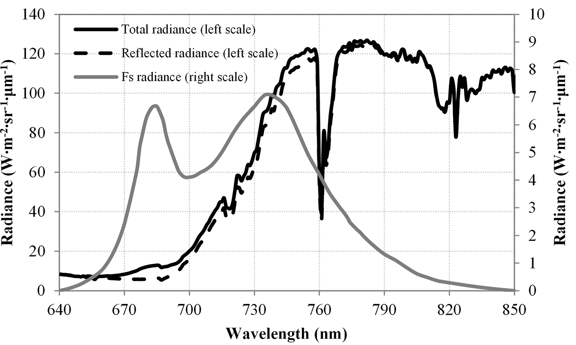
The total radiance of vegetation at wavelength λ, L(λ), can be expressed as a linear combination of the reflected radiance and the Fs radiance [1]:
2.2.2. Fs retrieval at Absorption Lines
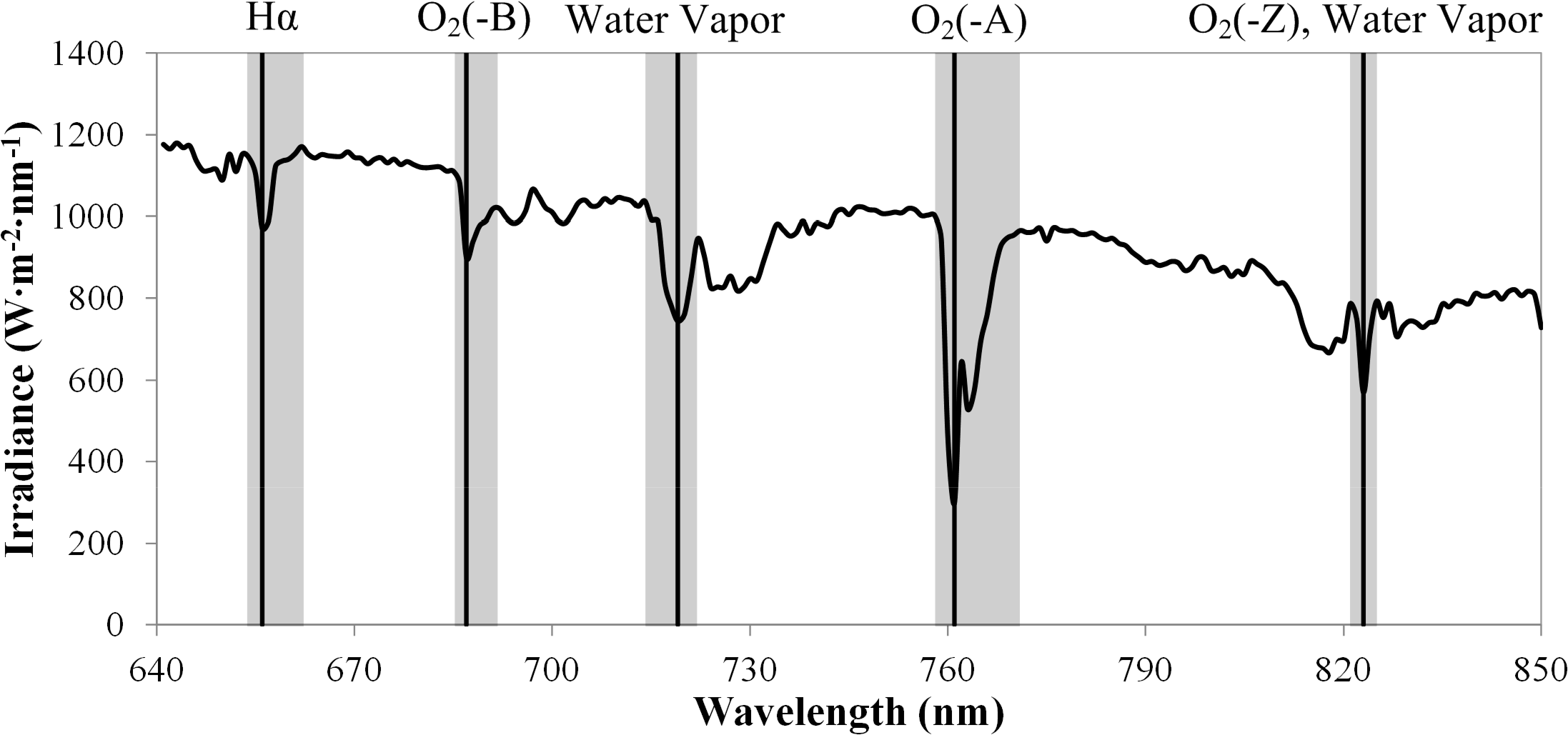
The first step of the FSR method is to retrieve the fluorescence radiance at the absorption lines within the Fs emission region of 640–850 nm. Five absorption lines were used for the fluorescence radiance retrieval [26]. The central wavelengths (spectral positions of the maximum absorption) and spectral ranges of these lines are shown in Figure 2 and summarized in Table 2. It should be noted that the Absorption Line 3 (Water vapor) originates from absorption by atmospheric water vapor, whose content fluctuates greatly with time and location. Therefore, this absorption line may not be so evident when air humidity is low. The lower and upper limits of each spectral range were determined according to the boundaries of the absorption well. In Figure 2, the incident solar irradiance spectrum at TOC was simulated by MODTRAN-5 [27] for a standard mid-latitude summer model atmosphere, and the default rural aerosol model. Both the SR and SSI of the spectrum are 1 nm.
The SFM method was used to estimate Fs at these five absorption lines. The underlying assumption of the SFM method is that the spectral variations of F(λ) and r(λ) can be described by appropriate mathematical functions in the pre-defined range around each absorption line [12]. In this study, for each absorption line we approximate the unknown F(λ) and r(λ) by Taylor polynomials, with the terms higher than second order being truncated:
In order to determine the six unknown coefficients, one needs at least six sampling values of L(λ) and E(λ) within each spectral range defined in Table 2.
In this study, all available sampling points (λ = λ1, λ2, …, λn) within each spectral range were used to construct the over-determined linear system:
Then, the vector of the six unknown coefficients (B) can be determined by the least squares method:
2.2.3. The Extraction of Basis Fs Spectra with the SVD Technique
The SVD was performed to extract several basis spectra that could describe the distribution of the Fs spectrum. The 1000 Fs spectra simulated by the model SCOPE (Dataset I) were used as training dataset with each of them containing 211 sampling points (SSI = 1 nm, within the Fs emission region of 640–850 nm). All the training spectra were arranged into a matrix A that contains 1000 rows (the number of Fs spectra) and 211 columns (number of sampling points in each spectrum). With the SVD method, A can be decomposed as a product of three matrices:
Generally, the larger the number of singular vectors were used, the more precisely the Fs spectrum can be reconstructed. However, at most five available Fs values at different absorption lines (Figure 2) can be retrieved to determine the coefficients of the singular vectors. If the number of singular vectors is larger than the number of the available Fs values, the linear system of Equation (10) to be solved in Section 2.2.4 will be underdetermined. As a compromise, three singular vectors (i.e., v1, v2, and v3) corresponding to the first three largest singular values were used in this study for reconstructing the Fs spectrum.
Then, the Fs spectrum (FFSR) could be calculated with a linear combination of the three singular vectors:
2.2.4. Determination of the Coefficients of Singular Vectors
The retrieved Fs values in the five wavelengths with the SFM method were denoted as F(656), F(687), F(719), F(761), and F(823), according to the absorption lines used to retrieve them. However, the retrieval accuracies of them are different. Generally, the more strongly absorbed line is more suitable for Fs retrieval, and consequently produces a lower condition number of MT × M when solving Equation (6). Therefore, for each Fs value we assign it a weight w(i) which could adjust the impact of its retrieval accuracy on the determination of the coefficients of the singular vectors. The weight equals the reciprocal of the condition number of MT × M.
Then, the coefficients (c1, c2, and c3) of the three singular vectors are determined by fitting the FFSR at the five absorption lines (computed by Equation (8)) to their correspondingly retrieved Fs values. The merit function f to determine c1, c2, and c3 is expressed as:
Determining c1, c2, and c3 by minimizing f is a WLLS problem whose solution is explicitly provided by [28]:
If one or more absorption lines are not deep enough (e.g., the Absorption Line 3 (Water vapor) under low humidity condition), their weights will decrease, and Fs values retrieved from these lines will play a smaller role when solving Equation (10). With the inverted values of c1, c2, and c3, one can reconstruct the Fs spectrum (FFSR) according to Equation (8).
2.3. Accuracy Evaluation
The simulated datasets generated by the SCOPE model (i.e., the Dataset II and III described in Section 2.1.1) were used in this study to evaluate the accuracy of the FSR method. In these datasets, the solar irradiance E(λ), the canopy up-welling radiance L(λ), and the Fs radiance F(λ) were simulated. Here, the simulated F(λ) was regarded as the “true” value, which would be used to validate the FFSR(λ) reconstructed with the FSR method. The coefficient of determination (R2) and Root-Mean-Square Error (RMSE) between the reconstructed FFSR(λ) and “true” F(λ) were calculated at 761 nm (central wavelength position of the Absorption Line 4 (O2-A)), 687 nm (central wavelength position of the Absorption Line 2 (O2-B)), 656 nm (central wavelength position of the Absorption Line 1 (Hα)), 699 nm (the approximate position of the middle valley of Fs spectrum), 684 nm (the approximate position of the left peak of Fs spectrum), and 736 nm (the approximate position of the right peak of Fs spectrum). The Fs integrated over the fluorescence emission bands of 640–850 nm were also compared between FFSR(λ) and F(λ) with R2 and RMSE. Meanwhile, the FSR method was also applied to the experimental dataset described in Section 2.1.2. Canopy Fs spectra from 8:00–18:00 were reconstructed from field hyperspectral measurements. Diurnal variations of the Fs spectra were analyzed to see if it was consistent with the former studies.
3. Results and Discussion
3.1. Extracted Singular Vectors
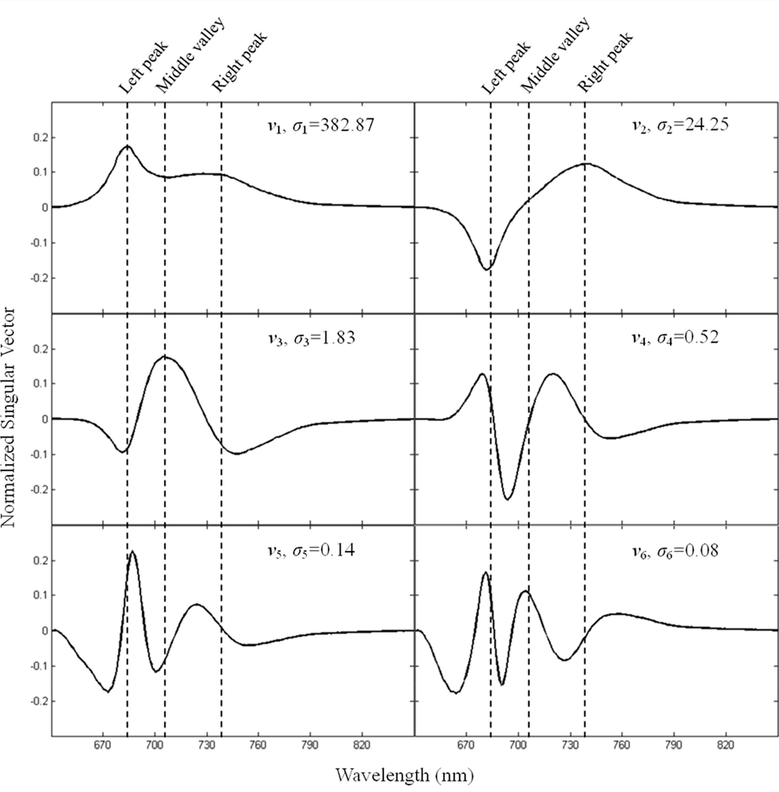
The first six singular vectors (v1, v2, …, v6) extracted from the training data (Dataset I) are shown in Figure 3, together with their corresponding singular values (σ1, σ2, …, σ6). The first singular vector v1 delineates the general shape of the Fs spectrum (Figure 3a). It corresponds to the largest singular value (σ1 = 382.87) and captures most of the variance in the training dataset (Dataset I). The second singular vector v2 can adjust the peak-difference of the Fs spectrum (Figure 3b). The third singular vector v3 controls the depth of the middle valley between the two peaks (Figure 3c). The remaining three singular vectors (with their singular value lower than 1) give limited and delicate information about the Fs spectrum (Figure 3d–f) and were ignored. Therefore, the first three singular vectors (i.e., v1, v2, and v3) were used to reconstruct the Fs spectrum.
3.2. Assessment of the FSR Method with Noise-Free Data
The FSR method was then evaluated with the noise-free dataset simulated by the SCOPE model (Dataset II). Figure 4 shows the scatter diagrams of retrieved versus “true” Fs values at 761 nm, 687 nm, 656 nm, 699 nm, 684 nm, and 736 nm. Results indicate that the reconstructed Fs values agree well with the “true” Fs values, with R2 values higher than 0.99 and RMSE values lower than 0.2 W∙m−2∙sr−1∙μm−1 at these six wavelengths.
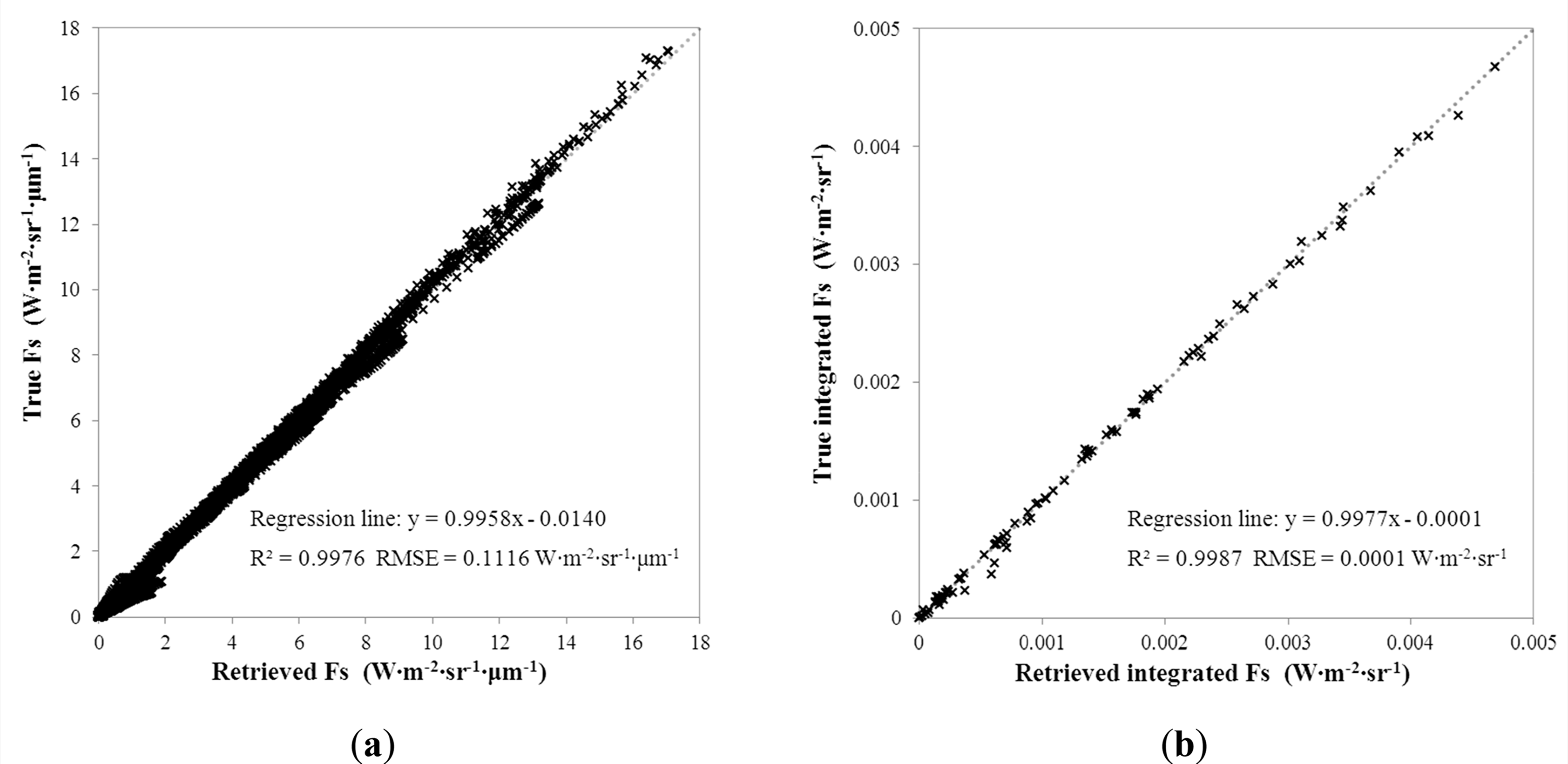
Figure 5a gives the scatter diagram of retrieved versus “true” Fs values at all wavelengths within the Fs emission region of 640–850 nm with 1 nm step, with a high R2 value (0.9976) and a low RMSE value (0.1116 W∙m−2∙sr−1∙μm−1). Figure 5b shows the scatter diagram of retrieved versus “true” Fs integrated over the Fs emission region from 640–850 nm. Similarly, a high R2 value (0.9987) and a low RMSE value (0.0001 W∙m−2∙sr−1·μm−1) were obtained, which indicates a good overall accuracy of the FSR method for the noise-free data.
3.3. Assessment of the FSR Method with Noisy and Different SR Data
The impact of sensor configuration on the performance of the FSR method was investigated. Two important sensor parameters affecting the retrieval accuracy of Fs, SR and SNR, were considered to generate the noisy and different SR data. A total of 15 different SR/SNR pairs were selected (Table 3), which can cover most of the configurations of the instruments used in ground experiments [24]. Among these pairs, SR = 3 nm and SNR = 4000 corresponds to the configuration of the ASD FieldSpec Pro spectrometer [24] used in this study for acquiring field data. For each pair of sensor parameters, 100 Fs spectra were reconstructed from Dataset III (noisy and different SR data). Statistics (R2 and RMSE) between the retrieved and “true” values are provided in Table 3 for Fs at 761 nm, 687 nm, 684 nm, 736 nm, 699 nm, and 656 nm, and the integrated Fs from 640–850 nm.
Results indicate that the accuracy of the FSR method is significantly affected by the sensor parameters (SR and SNR). It was found that a decrease of SR or/and SNR leads to a decrease of the retrieval accuracy of the Fs spectrum. For the pair of SR = 0.1 nm and SNR = 4000, which is the best sensor configuration considered, the accuracy was quite high with the R2 higher than 0.999 for the radiance at the six wavelengths and the integrated Fs, and RMSE lower than 0.021 W∙m−2∙sr−1∙μm−1 and 0.0011 W∙m−2∙sr−1, respectively. This indicates that the FSR method could achieve a rather high accuracy with instruments of high SR and SNR. However, for the poorest sensor configuration of SR = 3 nm and SNR = 300, rather poor results are obtained with the highest R2 of the Fs radiance at the Absorption Line 4 (O2-A) being only 0.4889. Besides, for the pair of SR = 3 nm and SNR = 4000 (corresponding to the configuration of the ASD FieldSpec Pro spectrometer), we obtain the statistics with R2 values higher than 0.8 and RMSE lower than 2.1 W∙m−2∙sr−1∙μm−1 at all six wavelengths, and R2 and RMSE of the integrated Fs being 0.9439 and 0.0892 W∙m−2∙sr−1, respectively, whose qualification of the accuracy is dependent on the user’s requirements.
3.4. Application of the FSR Method to the Experimental Dataset
The Fs spectra were reconstructed from the TOC incident irradiance and up-welling radiance acquired in the field experiment in 2010 [25]. Figure 6 shows the diurnal course of the reconstructed spectra. The shapes of the reconstructed Fs spectra are consistent with those from former studies [18,21]. The radiance values of the reconstructed Fs spectra at the Absorption Line 4 (O2-A) (about 1–3 W∙m−2∙sr−1∙μm−1) also compare well with the values reported in former studies [5,25,29,30]. It can be seen that for most of the reconstructed Fs spectra, the left peak is lower than the right one. Because the left peak of Fs is located within the spectral region of chlorophyll absorption, the reduction of its amplitude may be explained by the re-absorption effect caused by chlorophyll [31]. Moreover, a typical diurnal change of the reconstructed Fs spectra could be observed. During the morning as shown in Figure 6a, the Fs spectra (with intervals of 60 min) showed an increasing trend. During the afternoon, a decreasing trend was observed (Figure 6b). It was seen that the magnitude of the right peak of the Fs spectrum at 12:00 is not highest compared with those at 10:00 and 11:00, which probably resulted from the stress factors induced by excessive light and heat [32]. In the early morning and late afternoon (8:00 and 17:00–18:00), the Fs radiance was relatively low and less than 3 W∙m−2∙sr−1∙μm−1 in all wavelengths between 640 and 850 nm (Figure 6c). From mid-morning to mid-afternoon (10:00–15:00), the Fs radiance was relatively high (Figure 6c), which can be attributed to the increase of the incident irradiance. At 13:30, a significantly abnormal value of the right peak of the reconstructed Fs spectrum appeared, which needs further investigation.
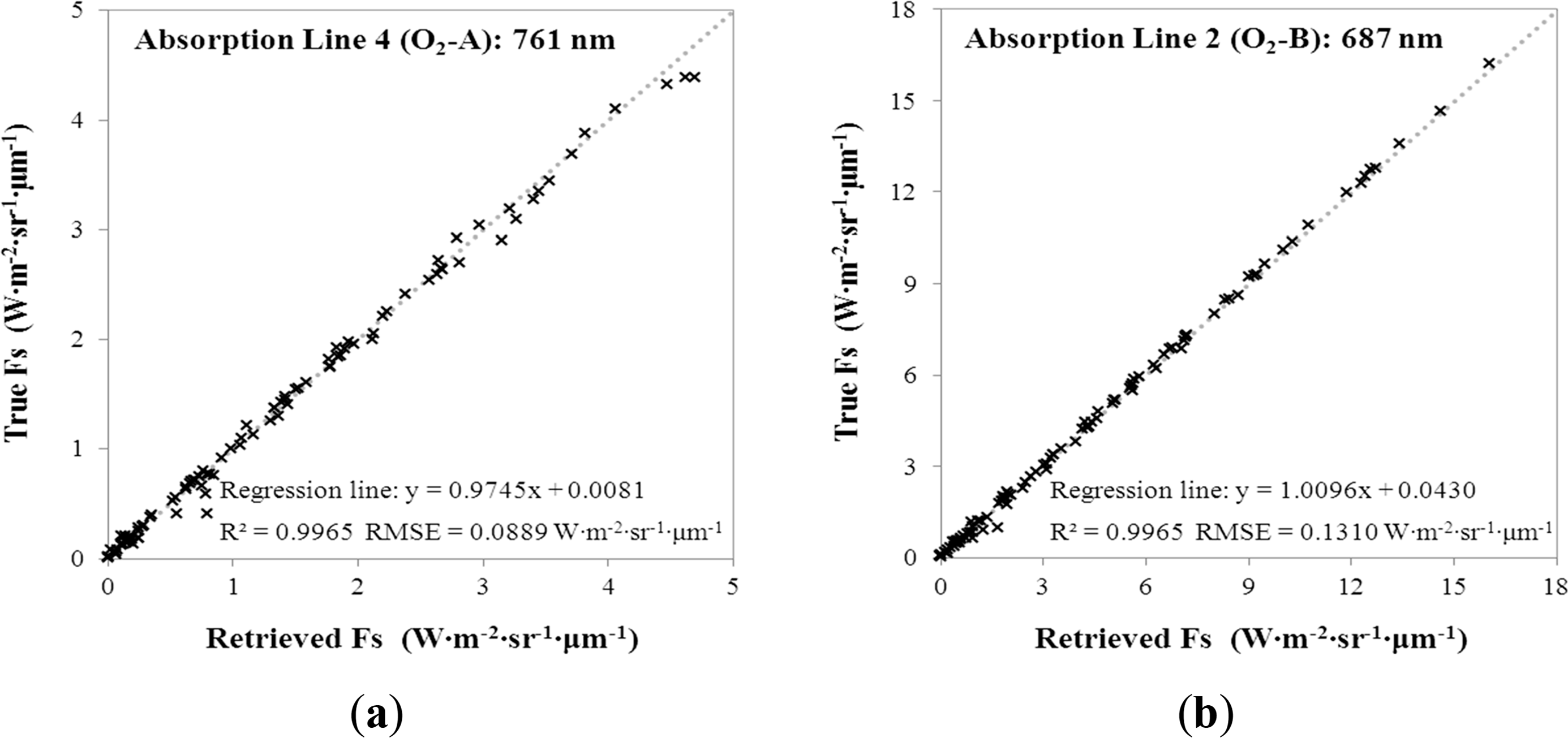
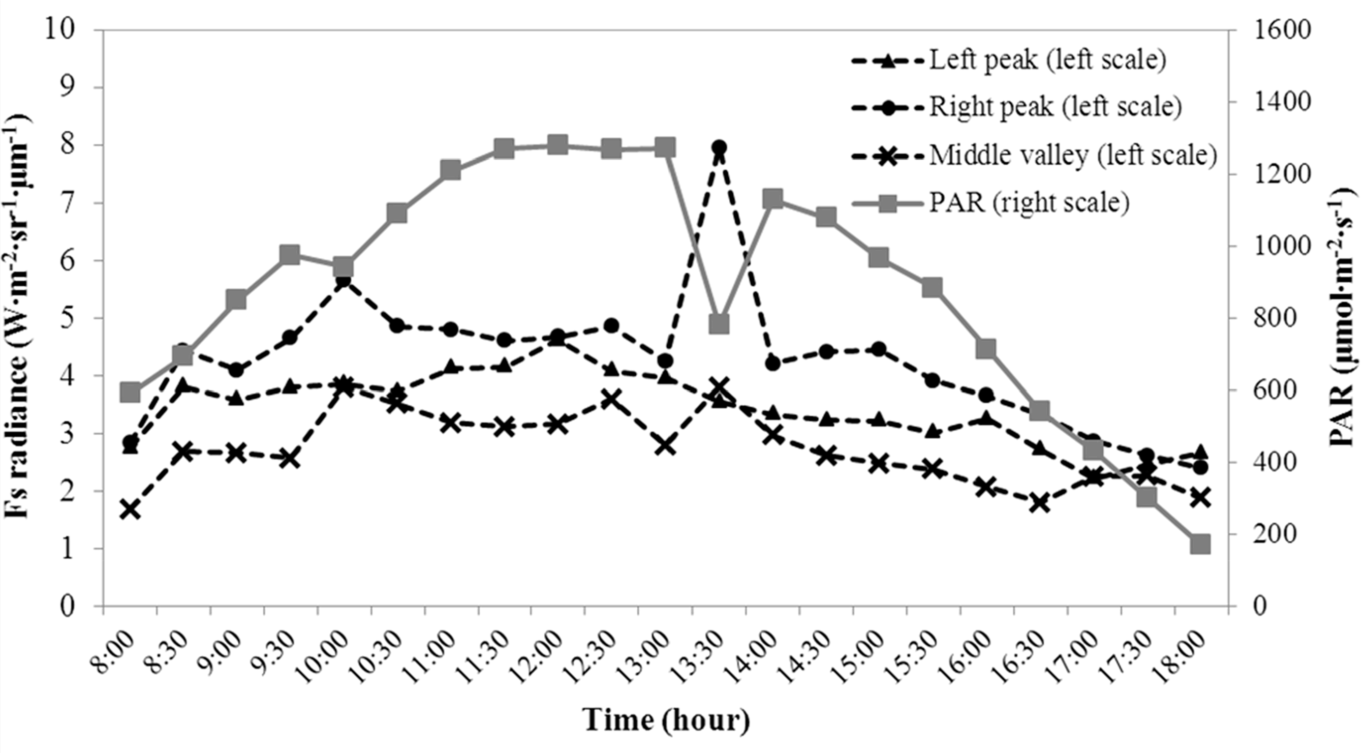
Figure 7 shows the diurnal courses of the solar-induced chlorophyll fluorescence (Fs) at 684 nm, 736 nm, and 699 nm, approximately the left and right peaks of the Fs spectrum, and the middle valley of the Fs spectrum, respectively. It can be seen that the magnitudes in Fs follow the diurnal course of PAR. This is consistent with the results reported in former studies, in which the Fs radiance retrieved from the Absorption Line 4 (O2-A) was shown to be closely correlated to the incident PAR [25,29]. The R2 values between PAR and Fs radiance (excluding the data points at 13:30) are 0.71, 0.70, and 0.56 for 684 nm, 761 nm, and 699 nm, respectively. The Fs values at the Absorption Line 4 (O2-A) and 2 (O2-B) retrieved by the FSR method are close to the results reported in [25], with R2 at both of the two bands higher than 0.96 and RMSE lower than 0.3 W∙m−2∙sr−1∙μm−1. These results suggest that the FSR method can be successfully applied for experimental datasets, and has potential for practical applications.
3.5. Limitations and Potential of the FSR Method
Two approximations were adopted in the FSR method. Firstly, F(λ) and r(λ) were approximated by quadratic functions in Equations (2) and (3), respectively. This approximation was induced by the SFM, which has been demonstrated to be rather reasonable [12]. It should be noted that the selection of the mathematical functions to approximate F(λ) and ρ(λ) may affect the performance of the SFM method in estimating Fs. We will investigate the impact of the choice of different mathematical functions to approximate the F(λ) and r(λ) on the retrieval accuracy of the Fs value for each absorption line, and finally on the accuracy of Fs spectrum reconstruction. Secondly, only the first three singular vectors were used to reconstruct the FFSR (Equation (8)). Because the singular vectors corresponding to the larger singular values (e.g., σ > 1) give more “global” information about the distribution of the Fs spectrum, and the singular vectors corresponding to smaller singular values (e.g., σ < 1) give more “detailed” information, this approximation would only lead to the loss of the small variations on the Fs spectrum. According to the results shown in Figure 3, the first three singular vectors contain the most meaningful information to control the general shape of Fs. With the decrease of singular values, their corresponding singular vectors contain more subtle information. This information may correspond to the specific cases related to the different environmental conditions, canopy structures, and leaf biochemical status, which should be embodied by the retrieved Fs spectrum for the measured data. On the other hand, constrained by a maximum of five available Fs values at the absorption lines, the first three singular vectors were used to reconstruct the Fs spectrum in this study.
For the extraction of the basis Fs spectra, a total of 1000 SCOPE-simulated Fs spectra were used as training data. When more Fs spectra (e.g., 1500) were included into the training dataset, the extracted singular vectors did not show noticeable difference from the singular vectors shown in Figure 3. Therefore, 1000 Fs spectra were found to be sufficient for a stable extraction of the basis Fs spectra in this study.
With the improvement of the sensor properties, the selection of the spectral range of each absorption line (as shown in Table 1) and the mathematical functions to characterize F(λ) and r(λ) (Equations (2) and (3)) can be further refined for the SFM method shown in Section 2.2.2, or other Fs retrieval methods with higher precision. This can improve the retrieval accuracies of the Fs values at the absorption lines, which in turn will improve the determination of the coefficients of singular vectors during the optimization process. As a result, the accuracy of the reconstructed Fs spectrum should be improved. However, field datasets acquired by sensors of higher SR and SNR than those of the ASD spectrometer used in this study are still needed to test the performance of the FSR method.
When reconstructing the Fs spectrum with three singular vectors for poor-quality field datasets (e.g., acquired by instrument of low SR and SNR and/or under unstable measuring conditions), the shape of the reconstructed Fs spectrum deviated from the typical two-peak distributions, and values of Fs were not in the reported ranges, which implied a failure of the reconstruction. The reason mainly lies in the inaccuracy of Fs retrieval for less wide and deep absorption lines. To make a reliable reconstruction of the Fs spectrum, only the more stable O2-A and O2-B lines should be used. Then, the number of singular vectors used to reconstruct the Fs spectrum (Equation (8)) should reduce to two (i.e., the first two singular vectors) to prevent Equation (10) from being underdetermined. Correspondingly, coefficients of the merit function (Equation (9)) reduce to two and can be determined. Results for this modified approach showed that both the shape and values of the reconstructed Fs spectrum are consistent with those in the literature. To further evaluate the performance of the FSR method and the modified approach, it is suggested that sensors, with both high and relatively low spectral properties covering the whole fluorescence emission range from 640–850 nm, simultaneously measure the same vegetated target under the same measuring conditions. Theoretically, the Fs spectrum reconstructed from the dataset obtained by the sensor of high spectral properties should be more accurate, and can be used to assess the accuracy for the sensor of low spectral properties. Hopefully, we will conduct this comparison in future studies.
The training dataset was simulated by the model SCOPE, which is a one-dimensional radiative transfer model suitable for horizontally homogeneous canopies. Although SCOPE can simulate BRDF effects related to the leaf angle distribution and the hot spot effect, the applicability of the FSR method trained by SCOPE needs further investigation for discontinuous canopies, such as row-planted crops, which show even more distinct features of bi-directional radiation transfer [33]. Moreover, in this study, the FSR method was only applied to ground measurements. Our future work will investigate how to extend this method to air-borne and space-borne data.
The FSR method proposed in this study provides researchers an overall view about the TOC Fs spectrum. It has demonstrated its potential to be used in future studies. For example, in previous studies, only Fs at specific absorption lines (e.g., the commonly used O2-A and O2-B lines) could be retrieved from ground measurements. Some meaningful parameters, such as the fluorescence peak-ratio and the information about the peak center, peak width of Fs, cannot be calculated in this way. With the Fs spectrum reconstructed by the FSR method, these parameters could be calculated and further applied for plant status monitoring. Moreover, the FSR method can also be used for the validation of canopy fluorescence radiative transfer models with field hyperspectral data.
4. Conclusions
We proposed a FSR method to reconstruct the solar-induced chlorophyll fluorescence spectrum over the whole fluorescence emission bands of 640–850 nm with hyperspectral measurements. Both simulated and experimental datasets were used in this study to assess the performance of the FSR method. Results indicate that the FSR method could successfully reconstruct the Fs spectrum from hyperspectral measurements. The analysis of the impact of the sensor parameters showed that an improvement of the SR and SNR could achieve a higher accuracy with the FSR method. For the experimental dataset, the diurnal variation of the reconstructed Fs spectra was observed, with the Fs radiance at noontime higher than that in the morning and afternoon. The characteristics of the reconstructed Fs spectra and the close relationship between PAR and Fs radiance were consistent with former studies. Results presented in this study demonstrate that the proposed FSR method can be used to retrieve continuous Fs spectra and has potential for future applications.
Acknowledgments
This work is jointly supported by the Chinese Natural Science Foundation under Project 41371325, the National Basic Research Program of China (973 Program) (Grant No: 2010CB950800), and the Civil Aerospace Technology Pre-research Project of China (Grant No. D040201-03). The authors are thankful to the anonymous reviewers who provided constructive comments to improve this manuscript.
Author Contributions
Feng Zhao conceived the research, proposed the research method, and made significant contributions in manuscript preparation and revision. Yiqing Guo conducted the data analysis and prepared the manuscript. Wout Verhoef provided the SCOPE model, and contributed extensively in the research method and the manuscript revision. Xingfa Gu provided suggestions for the research and manuscript revision. Liangyun Liu designed and conducted the field experiment, and provided suggestions for the manuscript revision. Guijun Yang provided the experimental conditions and facilities, and contributed to the manuscript revision.
Conflicts of Interest
The authors declare no conflict of interest.
References and Notes
- Meroni, M.; Rossini, M.; Guanter, L.; Alonso, L.; Rascher, U.; Colombo, R.; Moreno, J. Remote sensing of solar-induced chlorophyll fluorescence: Review of methods and applications. Remote Sens. Environ 2009, 113, 2037–2051. [Google Scholar]
- Malenovsky, Z.; Mishra, K.B.; Zemek, F.; Rascher, U.; Nedbal, L. Scientific and technical challenges in remote sensing of plant canopy reflectance and fluorescence. J. Exp. Bot 2009, 60, 2987–3004. [Google Scholar]
- Maier, S.W.; Günther, K.P.; Stellmes, M. Sun-induced fluorescence: A new tool for precision farming. In Digital Imaging and Spectral Techniques: Applications to Precision Agriculture and Crop Physiology; VanToai, T., Major, D., McDonald, M., Schepers, J., Tarpley, L., Eds.; American Society of Agronomy: Madison, WI, USA, 2003; pp. 209–222. [Google Scholar]
- Zarco-Tejada, P.J.; González-Dugo, V.; Berni, J.A.J. Fluorescence, temperature and narrow-band indices acquired from a UAV platform for water stress detection using a micro-hyperspectral imager and a thermal camera. Remote Sens. Environ 2012, 117, 322–337. [Google Scholar]
- Zarco-Tejada, P.J.; Catalina, A.; González, M.R.; Martín, P. Relationships between net photosynthesis and steady-state chlorophyll fluorescence retrieved from airborne hyperspectral imagery. Remote Sens. Environ 2013, 136, 247–258. [Google Scholar]
- Van Wittenberghe, S.; Alonso, L.; Verrelst, J.; Hermans, I.; Valcke, R.; Veroustraete, F.; Moreno, J.; Samson, R. A field study on solar-induced chlorophyll fluorescence and pigment parameters along a vertical canopy gradient of four tree species in an urban environment. Sci. Total Environ 2014. [CrossRef]
- Alonso, L.; Gómez-Chova, L.; Vila-Francés, J.; Amorós-López, J.; Guanter, L.; Calpe, J.; Moreno, J. Improved Fraunhofer Line Discrimination method for vegetation fluorescence quantification. IEEE Geosci. Remote Sens. Lett 2008, 5, 620–624. [Google Scholar]
- Plascyk, J.A.; Gabriel, F.C. The Fraunhofer Line Discriminator MKII—An airborne instrument for precise and standardized ecological luminescence measurements. IEEE Trans. Instrum. Meas 1975, 24, 306–313. [Google Scholar]
- Theisen, A.F. Detecting chlorophyll fluorescence from orbit: The Fraunhofer Line Depth model. In From Laboratory Spectroscopy to Remotely Sensed Spectra of Terrestrial Ecosystems; Muttiah, R.S., Ed.; Kluwer Academic Publishers: Dordrecht, The Netherlands, 2002; pp. 203–232. [Google Scholar]
- Gómez-Chova, L.; Alonso, L.; Amorós-López, J.; Vila-Francés, J.; del Valle-Tascón, S.; Calpe, J.; Moreno, J. Solar-induced fluorescence measurements using a field spectroradiometer. In Proceedings of the 2005 AIP Conference Proceedings Earth Observation for Vegetation Monitoring and Water Management, Naples, Italy, 10–11 November 2005; 852, pp. 274–281.
- Meroni, M.; Colombo, R. Leaf level detection of solar induced chlorophyll fluorescence by means of a subnanometer resolution spectroradiometer. Remote Sens. Environ 2006, 103, 438–448. [Google Scholar]
- Meroni, M.; Busetto, L.; Colombo, R.; Guanter, L.; Moreno, J.; Verhoef, W. Performance of spectral fitting methods for vegetation fluorescence quantification. Remote Sens. Environ 2010, 114, 363–374. [Google Scholar]
- Guanter, L.; Frankenberg, C.; Dudhia, A.; Lewis, P.E.; Gómez-Dans, J.; Kuze, A.; Suto, H.; Grainger, R.G. Retrieval and global assessment of terrestrial chlorophyll fluorescence from GOSAT space measurements. Remote Sens. Environ 2012, 121, 236–251. [Google Scholar]
- Guanter, L.; Rossini, M.; Colombo, R.; Meroni, M.; Frankenberg, C.; Lee, J-E; Joiner, J. Using field spectroscopy to assess the potential of statistical approaches for the retrieval of sun-induced chlorophyll fluorescence from ground and space. Remote Sens. Environ 2013, 133, 52–61. [Google Scholar]
- Hak, R.; Lichtenthaler, H.K.; Rinderle, U. Decrease of the fluorescence ratio F690/F730 during greening and development of leaves. Radiat. Environ. Biophys 1990, 29, 329–336. [Google Scholar]
- Pedrós, R.; Goulas, Y.; Jacquemoud, S.; Louis, J.; Moya, I. FluorMODleaf: A new leaf fluorescence emission model based on the PROSPECT model. Remote Sens. Environ 2010, 114, 155–167. [Google Scholar]
- Subhash, N.; Mohanan, C.N. Curve-fit analysis of chlorophyll fluorescence spectra: Application to nutrient stress detection in sunflower. Remote Sens. Environ 1997, 60, 347–356. [Google Scholar]
- Miller, J.R.; Berger, M.; Goulas, Y.; Jacquemoud, S.; Louis, J.; Moise, N.; Mohammed, G.; Moreno, J.; Moya, I.; Pedrós, R.; et al. Development of a Vegetation Fluorescence Canopy Model; Final Report; European Space Research and Technology Centre (ESTEC): Noordwijk, The Netherlands, 2005. [Google Scholar]
- Van Wittenberghe, S.; Alonso, L.; Verrelst, J.; Verrelst, I.; Delegido, J.; Veroustraete, F.; Veroustraete, R.; Moreno, J.; Samson, R. Upward and downward solar-induced chlorophyll fluorescence yield indices of four tree species as indicators of traffic pollution in Valencia. Environ. Pollut 2013, 173, 29–37. [Google Scholar]
- Verhoef, W. Light scattering by leaf layers with application to canopy reflectance modeling: The SAIL model. Remote Sens. Environ 1984, 16, 125–141. [Google Scholar]
- Van der Tol, C.; Verhoef, W.; Timmermans, J.; Verhoef, A.; Su, Z. An integrated model of soil-canopy spectral radiances, photosynthesis, fluorescence, temperature and energy balance. Biogeosciences 2009, 6, 3109–3129. [Google Scholar]
- Zhao, F.; Huang, Y.; Guo, Y.; Reddy, K.N.; Lee, M.A.; Fletcher, R.S.; Thomson, S.J. Early detection of crop injury from glyphosate on soybean and cotton using plant leaf hyperspectral data. Remote Sens 2014, 6, 1538–1563. [Google Scholar]
- Feret, J.B.; François, C.; Asner, G.P.; Gitelson, A.A.; Martin, R.E.; Bidel, L.P.; Ustin, S.L.; le Maire, G.; Jacquemoud, S. PROSPECT-4 and 5: Advances in the leaf optical properties model separating photosynthetic pigments. Remote Sens. Environ 2008, 112, 3030–3043. [Google Scholar]
- Damm, A.; Erler, A.; Hillen, W.; Meroni, M.; Schaepman, M.E.; Verhoef, W.; Rascher, U. Modeling the impact of spectral sensor configurations on the FLD retrieval accuracy of sun-induced chlorophyll fluorescence. Remote Sens. Environ 2011, 115, 1882–1892. [Google Scholar]
- Liu, L.; Zhang, Y.; Jiao, Q.; Peng, D. Assessing photosynthetic light-use efficiency using a solar-induced chlorophyll fluorescence and photochemical reflectance index. Int. J. Remote Sens 2013, 34, 4264–4280. [Google Scholar]
- Meroni, M.; Busetto, L.; Guanter, L.; Cogliati, S.; Crosta, G.F.; Migliavacca, M.; Panigada, C.; Rossini, M.; Colombo, R. Characterization of fine resolution field spectrometers using solar Fraunhofer lines and atmospheric absorption features. Appl. Opt 2010, 49, 2858–2871. [Google Scholar]
- Berk, A.; Anderson, G.P.; Acharya, P.K.; Chetwynd, J.H.; Bernstein, L.S.; Shettle, E.P.; Matthew, M.W.; Adler-Golden, S.M. MODTRAN-4 User’s Manual; Air Force Research Laboratory: Bedford, MA, USA, 2000. [Google Scholar]
- Strutz, T. Data Fitting and Uncertainty: A Practical Introduction to Weighted Least Squares and Beyond; Vieweg and Teubner: Amsterdam, The Netherlands, 2010. [Google Scholar]
- Liu, L.; Zhang, Y.; Wang, J.; Zhao, C. Detecting solar-induced chlorophyll fluorescence from field radiance spectra based on the Fraunhofer Line Principle. IEEE Trans. Geosci. Remote Sens 2005, 43, 827–832. [Google Scholar]
- Zarco-Tejada, P.J.; Suárez, L.; González-Dugo, V. Spatial resolution effects on chlorophyll fluorescence retrieval in a heterogeneous canopy using hyperspectral imagery and radiative transfer simulation. IEEE Geisci. Remote Sens. Lett 2013, 10, 937–941. [Google Scholar]
- Buschmann, C. Variability and application of the chlorophyll fluorescence emission ratio red/far-red of leaves. Photosynth. Res 2007, 92, 261–271. [Google Scholar]
- Amoros-Lopez, J.; Gomez-Chova, L.; Vila-Frances, J.; Alonso, L.; Calpe, J.; Moreno, J.; del Valle-Tascon, S. Evaluation of remote sensing of vegetation fluorescence by the analysis of diurnal cycles. Int. J. Remote Sens 2008, 29, 5423–5436. [Google Scholar]
- Zhao, F.; Gu, X.; Verhoef, W.; Wang, Q.; Yu, T.; Liu, Q.; Huang, H.; Qin, W.; Chen, L.; Zhao, H. A spectral directional reflectance model of row crops. Remote Sens. Environ 2010, 114, 265–285. [Google Scholar]


| Parameter | Definition | Unit | Range |
|---|---|---|---|
| Leaf | |||
| N | Leaf structure parameter | - | 1–2.5 |
| Cab | Chlorophyll a+b content | μg∙cm−2 | 0.4–76.8 |
| Cw | Water content | g∙cm−2 | 0.0044–0.0340 |
| Cm | Dry matter content | g∙cm−2 | 0.0017–0.0331 |
| Vcmo | Maximum carboxylation capacity | umol∙m−2∙s−1 | 20–40 |
| Type | Photochemical pathway | - | 0 (C3) or 1 (C4) |
| fqe | Fluorescence quantum yield efficiency at photosystem level | - | 0–0.02 |
| Canopy | |||
| LAI | Leaf area index | - | 0–6 |
| hc | Vegetation height | m | 0.2–5 |
| LIDFa | Leaf Inclination Distribution Function (LIDF) parameter a | - | −1–1 * |
| LIDFb | LIDF parameter b | - | −1–1 * |
| leafwidth | Leaf width | m | 0.05–0.2 |
| Soil | |||
| spectrum | Type of soil reflectance spectrum | - | 1 (type 1), 2 (type 2) or 3 (type 3) |
| Meteorology | |||
| Rin | Broadband incoming shortwave radiation (0.4–2.5 um) | W∙m−2 | 200–1600 |
| Ta | Air temperature | °C | 10–30 |
*The restriction |LIDFa| + |LIDFb| ≤ 1 is applied when generating the values of LIDFa and LIDFb.
| Index of the Absorption Line | Element | Central Wavelength (nm) | Spectral Range (nm) |
|---|---|---|---|
| 1 | Hα | 656 | 653–662 |
| 2 | O2(-B) | 687 | 683–692 |
| 3 | Water Vapor | 719 | 714–722 |
| 4 | O2(-A) | 761 | 757–771 |
| 5 | O2(-Z), Water Vapor | 823 | 819–825 |
| Sensor Parameters | Absorption Line 4 (O2-A): 761 nm | Absorption Line 2 (O2-B): 687 nm | Left Peak: 684 nm | Right Peak: 736 nm | Middle Valley: 699 nm | Absorption Line 1 (Hα): 656 nm | Integrated Fs (from 640 nm to 850 nm) | |||||||
|---|---|---|---|---|---|---|---|---|---|---|---|---|---|---|
| R2 | RMSE a | R2 | RMSE a | R2 | RMSE a | R2 | RMSE a | R2 | RMSE a | R2 | RMSE a | R2 | RMSE b | |
| SR = 0.1 nm SNR = 4000 | 0.9996 | 0.0096 | 0.9998 | 0.0158 | 0.9998 | 0.0202 | 0.9996 | 0.0192 | 0.9995 | 0.0185 | 0.9998 | 0.0013 | 0.9998 | 0.0011 |
| SR = 0.1 nm SNR = 1000 | 0.9994 | 0.0108 | 0.9994 | 0.0309 | 0.9993 | 0.0375 | 0.9988 | 0.0291 | 0.9953 | 0.0545 | 0.9994 | 0.0034 | 0.9991 | 0.0027 |
| SR = 0.1 nm SNR = 300 | 0.9971 | 0.0249 | 0.9958 | 0.0897 | 0.9951 | 0.1048 | 0.9946 | 0.0605 | 0.9727 | 0.1384 | 0.9957 | 0.0071 | 0.9950 | 0.0061 |
| SR = 0.3 nm SNR = 4000 | 0.9988 | 0.0287 | 0.9996 | 0.0475 | 0.9994 | 0.0605 | 0.9989 | 0.0577 | 0.9984 | 0.0554 | 0.9996 | 0.0038 | 0.9995 | 0.0034 |
| SR = 0.3 nm SNR = 1000 | 0.9983 | 0.0324 | 0.9984 | 0.0927 | 0.9979 | 0.1124 | 0.9964 | 0.0872 | 0.9858 | 0.1636 | 0.9984 | 0.0101 | 0.9972 | 0.0080 |
| SR = 0.3 nm SNR = 300 | 0.9912 | 0.0747 | 0.9876 | 0.2680 | 0.9853 | 0.3143 | 0.9837 | 0.1814 | 0.9182 | 0.4153 | 0.9875 | 0.0213 | 0.9851 | 0.0184 |
| SR = 1 nm SNR = 4000 | 0.9959 | 0.0958 | 0.9987 | 0.1582 | 0.9983 | 0.2017 | 0.9962 | 0.1924 | 0.9948 | 0.1845 | 0.9986 | 0.0126 | 0.9984 | 0.0113 |
| SR = 1 nm SNR = 1000 | 0.9942 | 0.1079 | 0.9947 | 0.3089 | 0.9933 | 0.3745 | 0.9881 | 0.2905 | 0.9528 | 0.5454 | 0.9948 | 0.0336 | 0.9905 | 0.0268 |
| SR = 1 nm SNR = 300 | 0.9706 | 0.2489 | 0.9587 | 0.8966 | 0.9510 | 1.0476 | 0.9458 | 0.6045 | 0.7273 | 1.3844 | 0.9583 | 0.0710 | 0.9504 | 0.0612 |
| SR = 2 nm SNR = 4000 | 0.9914 | 0.1312 | 0.9921 | 0.4996 | 0.9905 | 0.6601 | 0.9904 | 0.3728 | 0.9750 | 0.6096 | 0.9922 | 0.0368 | 0.9938 | 0.0272 |
| SR = 2 nm SNR = 1000 | 0.9583 | 0.2799 | 0.9581 | 0.8901 | 0.9515 | 1.0578 | 0.9328 | 0.8087 | 0.7661 | 1.7645 | 0.9567 | 0.0712 | 0.9418 | 0.0792 |
| SR = 2 nm SNR = 300 | 0.8899 | 0.4711 | 0.7233 | 3.3787 | 0.6656 | 4.1739 | 0.4976 | 2.5825 | 0.1561 | 6.4125 | 0.7290 | 0.2630 | 0.5761 | 0.2755 |
| SR = 3 nm SNR = 4000 c | 0.9860 | 0.1600 | 0.9008 | 1.8341 | 0.8852 | 2.0662 | 0.9524 | 0.6289 | 0.8092 | 1.6939 | 0.9039 | 0.1441 | 0.9439 | 0.0892 |
| SR = 3 nm SNR = 1000 | 0.9004 | 0.4508 | 0.8299 | 2.4794 | 0.7797 | 3.0991 | 0.6114 | 2.0755 | 0.1831 | 5.6123 | 0.8307 | 0.1946 | 0.6482 | 0.2293 |
| SR = 3 nm SNR = 300 | 0.4889 | 1.5501 | 0.1841 | 9.1544 | 0.0964 | 10.8787 | 0.1941 | 8.7311 | 0.0829 | 20.9382 | 0.2092 | 0.7364 | 0.1970 | 0.9382 |
ain units of W·m−2·sr−1·μm−1.bin units of W·m−2·sr−1;ccorresponding to the configuration of the ASD FieldSpec Pro spectrometer used in this study for acquiring
© 2014 by the authors; licensee MDPI, Basel, Switzerland This article is an open access article distributed under the terms and conditions of the Creative Commons Attribution license (http://creativecommons.org/licenses/by/4.0/).
Share and Cite
Zhao, F.; Guo, Y.; Verhoef, W.; Gu, X.; Liu, L.; Yang, G. A Method to Reconstruct the Solar-Induced Canopy Fluorescence Spectrum from Hyperspectral Measurements. Remote Sens. 2014, 6, 10171-10192. https://0-doi-org.brum.beds.ac.uk/10.3390/rs61010171
Zhao F, Guo Y, Verhoef W, Gu X, Liu L, Yang G. A Method to Reconstruct the Solar-Induced Canopy Fluorescence Spectrum from Hyperspectral Measurements. Remote Sensing. 2014; 6(10):10171-10192. https://0-doi-org.brum.beds.ac.uk/10.3390/rs61010171
Chicago/Turabian StyleZhao, Feng, Yiqing Guo, Wout Verhoef, Xingfa Gu, Liangyun Liu, and Guijun Yang. 2014. "A Method to Reconstruct the Solar-Induced Canopy Fluorescence Spectrum from Hyperspectral Measurements" Remote Sensing 6, no. 10: 10171-10192. https://0-doi-org.brum.beds.ac.uk/10.3390/rs61010171