Small Footprint Full-Waveform Metrics Contribution to the Prediction of Biomass in Tropical Forests

Abstract

We tested metrics from full-waveform (FW) LiDAR (light detection and ranging) as predictors for forest basal area (BA) and aboveground biomass (AGB), in a tropical moist forest. Three levels of metrics are tested: (i) peak-level, based on each return echo; (ii) pulse-level, based on the whole return signal from each emitted pulse; and (iii) plot-level, simulating a large footprint LiDAR dataset. Several of the tested metrics have significant correlation, with two predictors, found by stepwise regression, in particular: median distribution of the height above ground (nZ_median) and fifth percentile of total pulse return intensity (i_tot_5th). The former contained the most information and explained 58% and 62% of the variance in AGB and BA values; stepwise regression left us with two and four predictors, respectively, explaining 65% and 79% of the variance. For BA, the predictors were standard deviation, median and fifth percentile of total return pulse intensity (i_tot_stdDev, i_tot_median and i_tot_5th) and nZ_median, whereas for AGB, only the last two were used. The plot-based metric showed that the median height of echo count (HOMTC) performs best, with very similar results as nZ_median, as expected. Cross-validation allowed the analysis of residuals and model robustness. We discuss our results considering our specific case scenario of a complex forest structure with a high degree of variability in terms of biomass.

1. Introduction

The ability of recent LiDAR sensors to record the full-waveform (FW) has inspired discussion amongst the scientific community on what is the effective advantage that this data can contribute with respect to standard discrete-return (DR) LiDAR data. Numerous related investigations argue the pros and cons [1], but all agree on improvements from FW related to two aspects: (i) improved detection of weak return echoes, which results in an increase in overall point density [2] by a factor of two over high vegetation [3]; and (ii) metrics extracted from the distribution of the return energy E_i over time f(t_i) in the FW (e.g., amplitude, echo width, backscatter cross-section, backscatter cross-section per illuminated area and backscatter coefficient). Both DR and FW LiDAR data have proven to be popular among scientists dealing with natural resources on the Earth’s surface, in particular high vegetation (i.e., forests) due to the unique capability of penetrating the canopy structure [4]. Regarding forest’s structural characteristics, aboveground biomass (AGB), or the total mass above the ground of living tissues, and basal area (BA) are most useful for ecologists, bio-geochemists, foresters and policymakers [5]. Studies have shown that forest canopy structure metrics (specifically height and crown cover) are highly correlated with AGB: [6–8] are representative examples from a wide array of literature. Models that estimate these characteristics in tropical forests using remote sensing data were widely investigated, using passive and active optical sensors [9–13], as well as using a combination of DR LiDAR and hyperspectral [14]. DR only data were tested for efficacy in the estimation of volume and AGB in several forest types. The volume of uneven-aged forest with conifers was tested against twenty predictor metrics, where estimation at 40-m size pixels shows an R-squared of 0.75 using the mean of the first echo height distribution and the median of the second echo height distribution [15]. This is in line with other works [16–18] that use DR metrics related to canopy height distribution and canopy density; the latter is defined as the proportion of echoes in the various height percentiles in a plot (10%, 50% and 90%). Results vary from an R-squared of 0.75 to 0.94, depending on the complexity of the forest structure. Such metrics have also been used in [19], where different regression methods were tested to find the best combination of predictors avoiding collinearity. Non-tropical scenarios also give similar results when LiDAR metrics are used for AGB estimation; with a single-tree-based approach training areas in a pine plantation, [20] reported a coefficient of correlation that reached a value of 0.82 between actual and predicted AGB.

FW systems record the entire time-varying energy of the return signal from all illuminated surfaces; therefore, they return detailed information on canopy structure and distribution. Early investigations on FW data were done with large footprint sensors. Data from the SLICER sensor were used successfully to predict 91% of the variance in AGB in Douglas fir and western hemlock forests using canopy filled canopy volume and canopy height metrics; the former actually resulted in being the most important variable for predicting total AGB [7]. The spaceborne sensor, GLAS (Geoscience Laser Altimeter System), on-board ICESat (Ice, Cloud and Land Elevation Satellite), was used successfully to extract biomass via height metrics over large spatial scales [21,22].

FW metrics from large footprint LiDAR in tropical wet forests have resulted in significant R-squared values at the plot level, of 0.93 and 0.72, respectively, for AGB and BA [23]. The authors argue that small footprint (i.e., less than a 1-m diameter) pulses, compared to large footprint pulses, have a lower probability of hitting treetops and a lower probability of getting echoes from the ground in the case of very dense canopies. We believe that these limitations become less significant as the point density increases and that significant correlation can be obtained from small footprint waveform metrics with the necessary precautions. In small footprint FW, amplitude, width and other derived metrics, like decay rate [24] and the rise and fall time of the signal [25], significantly contribute towards improving the results of estimations related to leaf area density and classification of forest cover, respectively. An overview of other approaches that use FW data to extract forest parameters is reviewed in [26]. Another recent review dedicated to LiDAR for forests that discusses the latest developments of this technology is [27]. A common result, in all of the investigations that were mentioned, is the importance of metrics regarding height distributions, both in DR and in FW LiDAR data, and also the metrics that regard canopy density (e.g., the filled canopy volume). This stimulates us to investigate further methods that use FW LiDAR data to extract information in forests with structurally complex conditions, such as in our dataset.

The objective of this investigation is to evaluate and discuss the degree of correlation between LiDAR FW metrics from a small footprint airborne laser scanner and structural characteristics in West African tropical forests to estimate AGB and BA. The paper is organized as follows: (i) we provide a brief background on LiDAR applications for estimating AGB in tropical forests and highlight some differences between existing systems; (ii) we describe our study site and the dataset that was used; (iii) we present the method and the results of using only direct FW metrics and of adding derived height metrics; and (iv) we finally discuss results in relation to other efforts to estimate tropical forest structure and future developments of the research.

2. Data and Methods

2.1. Study Area

The study area considered in this research is located in the Upper Guinean Forest Belt, in the south-western Ghana forested tropical zone, and is composed of two protected areas: the Dadieso Forest Reserve (FR) and the Bia Conservation Area. Dadieso FR has a vegetation that is transitional between the moist evergreen and wet evergreen types. However, swampy areas are common throughout the forest and, in certain areas, cover hundreds of hectares. Although logging is not officially allowed in Dadieso, the forest is disturbed and degraded in many areas. It is surrounded by cocoa farms and small rural villages, and information provided by the Forestry Commission suggests these two elements strongly contribute to the illegal logging occurring in the reserve. The Bia Conservation Area comprises the Bia National Park (NP, northern part) and the Bia Resource Reserve (RR, southern part). The Bia Conservation Area covers the transition between two of Ghana’s forest types, moist evergreen forest in the south and moist semi-deciduous forests in the north [28]. In Bia National Park, no systematic logging activity occurred in the past, while selective logging was relatively intense in Bia Resource Reserve. Figure 1 shows the area over different scales of representation.

2.2. Field Data

The ground survey was conducted in 2012–2013 and established 40 plots of a 1600 m² area along the latitudinal gradient from the southern portion of Dadieso FR, through Bia RR to the northern part of Bia NP. Information on species, the diameter at breast height (DBH) and height was collected in the whole plot area for trees with DBH > 20 cm and in 400-m² subplots for trees with DBH > 5 cm (see

Table 1. Plot characteristics with the frequency distribution of the count of LiDAR echoes.

Characteristic	Value
Area per plot	1600 m2
Number of plots	40
Number of pulses per plot:
- mean(standard deviation)	8353 (1334)
- min/max	6245/12,380
Number of echoes per plot:
- mean(standard deviation)	10,403 (1724)
- min/max	7808/13,200
Relative flying height min-max	558 m–621 m
Measured Forest Parameters 1 Mean (σ)–min/max
Hm, tree heights (m)	14.4 (6.6)–2.7/49.0
DBH, diameter at breast height (m)	0.3 (0.226)–0.10/1.37
BA, basal area (m2·ha−1) 2	3.6 (2.2)–0.3/9.6
AGB, aboveground biomass (Mg·ha−1) 2,3	170 (112)–5.8/475.7

¹Measured for all trees having DBH > 5 cm; σ = standard deviation;²BA and AGB were calculated for each plot, and values were standardized to one hectare;³using the Chave equation for moist forests [5].

for the characteristics and Figure 1 for the detail of a plot over a very high resolution image). Only 1600-m² plots were used, even if the other thirty-nine 500-m² plots and fifteen 400-m² plots were available, to avoid critical problems related to plot size. All were identified and georeferenced with GNSS receivers with post-processing differential correction with fixed and float solutions, which provided us with sub-meter precision [29]. In the case of float solutions, we double checked that the canopy shape respects the vegetation characteristics using very high resolution (0.1 m) (Figure 1, bottom right window) images acquired in the same mission [14].

2.3. LiDAR Dataset

An aircraft equipped with a LiDAR sensor, the Optech Ltd. ALTM GEMINI (Helica srl., Amaro, Italy), flew over the study area in March 2012. The sensor includes a 1064-nm wavelength laser emitting at 167-kHz max pulse repetition frequency (PRF) and 0.25-mrad (1/e) beam divergence, as well as a waveform digitizer with 8-bit resolution sampling every 1 ns and with a 70-kHz max acquisition rate. The operational emitted pulse frequency gave a real minimum density inside the plots of 11 points per square meter. The digitizer recorded every other pulse, due to the limitation in the acquisition rate above reported, thus half of the points have FW information. The average beam width of the laser cone that reaches the canopy and the terrain surface at that flight height is ∼0.15 m. The swath of the LiDAR strip on the ground is 280 m. The sample plots are located at the center of two strips. For this reason, the maximum scan angle of the laser beam in the plots is never above 11°. This allows considering as not significant the influence of the scan angle in the value of the FW metrics [30].

The files with corrected sensor data (CSD) and digitizer data (NDF) were processed by the authors using C++ routines developed at the University of Padova for the 3D representation of FW data in forests [31]. FW data and the relative georeferenced information from each waveform sample in the NDF file are used to subset only signals falling inside the plots. Functions for positioning the return echoes are also derived from the work of [32] and [33]. The processing steps for extracting the FW information are reported in detail in the following section.

3. Methods

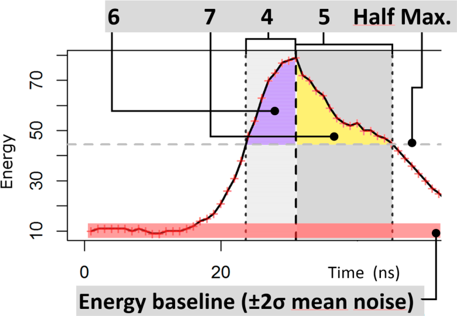
We extract FW metrics, which can be included in the following three different categories: (i) metrics associated with each return echo; (ii) metrics relative to the whole emitted pulse, e.g., total return energy; and (iii) aggregated metrics to simulate a large footprint laser beam.

Table 2. LiDAR metrics tested for correlation.

Extracted Metrics
Peak-Based
(1) Echo peak number	(En)
(2) Total echoes returned from pulse	(NoE)
(3) Normalized energy of peak	(i_peak)
(4) Left width	(LW)
(5) Right width	(RW)
(6) Left energy of peak	(LE)
(7) Right energy of peak	(RE)
(8) Height above ground	(nZ)
Pulse-Based
(9) Sampled signal above baseline	(NoANS)
(10) Total energy above baseline	(i_tot)
(11) Rise time	(RT)
(12) Fall time	(FT)
(13) Last peak energy	(LpE)
(14) Range * of median energy	(ROME)
(15) Range * of 3rd quartile energy	(RO3QE)
(16) Range * first to last peak	(rangefl)
(17) Ratio [ROME/LpE]	(RLER)
(18) Last return ratio [LpE/i_tot]	(LRR)
Large Footprint Simulation
(19) Height of median energy [23]	(HOME)
(20) Height of median target count	(HOMTC)
(21) Height/median ratio [23]	(HTRT)
(22) Ground return ratio [23]	(GRND)

^*In time bins of 1 ns, equivalent to ∼15 cm.

reports the list in each category and the corresponding numerical index and acronym used throughout the paper to refer to each metric. Figure 2 reports a schematic representation of the metrics related to a real example of the FW return signal; numbers in the figure are related to Table 2, and “Half Max” refers to half of the peak energy above the energy baseline, which is used to calculate the left and right width, which together are usually referred to as the full width at half maximum (FWHM).

In this article, we use the terms, echo and peak, as synonyms, as the peak represents the return echo in the FW signal, and each term fits in a particular sentence context. We therefore proceed to test for correlation eight metrics related to each return echo, ten metrics related to the whole return pulse, two of which are derived (17 and 18), and four large footprint simulation metrics. To test the relationship between metrics in Table 2 and the forest variables listed in Table 1, we aggregate each metric at the plot level and then use the measurements that were taken in the ground-truth campaign to fit models with multiple linear regression We use the following conventional descriptors of frequencies of distributions as aggregators: median, standard deviation, 5th and 95th percentiles. We choose percentiles instead of mean, minimum and maximum values, as extreme values and outliers have minor influence on their values.

3.1. Peak Detection

Peaks are detected with a threshold maxima approach [34] (see Equation 1, which represents a fast and effective algorithm [2], which was used in this approach). A total of 435,719 echoes are recorded for the 40 plots using this method, with a mean number of ∼10,000 points per plot. To define a peak, the following criteria are used:

$$p_t=\{\begin{array}{cc}1& E_{(t)}>E_{(t-1\dots i)}\hspace{0.17em}\mathit{and}\hspace{0.17em}{E}_{(t)}>E_{(t+1\dots i)}\\ 0& \mathit{otherwise}\end{array}$$

(1)

where p_t is the peak defined at time t in the waveform signal, E_(t) is the energy value recorded by the digitizer as time t, t is the time bin of 1 ns, which is equivalent to a distance of ∼0.15 m, and i is the time window threshold that is at least equal to the maximum width, where a local maximum can be mistaken as a peak due to noise. Several other sophisticated methods exist for peak detection and FW decomposition in the literature. We choose this specific approach that has proven to be effective and robust with a fast time of processing.

3.2. Metrics Extraction

The next step is to define the metrics listed in Table 2. The type of considered metrics allow dividing them into three categories: peak metrics, pulse metrics and large footprint-derived metrics. Full waveform metrics describe the surface response using the amplitude and width of the return signal’s energy distribution at each peak. The return energy E_i is influenced by the following factors other than emitted energy E₀ and surface response: atmospheric attenuation, range, footprint size relative to target area, multiple targets and geometry of laser beam and target [35,36]. We calculate normalized return energy E^N_i using the distance representing the range from the emitter, D_i against a nominal distance D₀ and a coefficient k amounting to a value of 2, as in the following equation:

$$E_i^N=\raisebox{1ex}{$\left(E_i\cdot D_i^k\right)$}\!\left/ \!\raisebox{-1ex}{$\left(E_0\cdot D_0^k\right)$}\right.$$

(2)

The literature identifies the backscattering coefficient γ (m²·m⁻²) and cross-section σ (m²) for describing and analyzing the scattering properties of targets [37]. Our study area is forested, and the investigation focuses on vegetation; therefore, we adopted the cross-section (σ) values. As explained in [35], if one deals with targets that are smaller than the size of the laser footprint (such as in forests), the target scattering area relevant for explaining σ remains the same, independent of the size of the laser footprint area (i.e., as long as the target is small compared to the footprint).

3.2.1. Peak Metrics

We extracted some descriptors derived from the part of the signal that is defined at half of the peak energy, i.e., the full width at half maxima (FWHM), which is divided into two components, left and right width (LW and RW). The respective integrated energy in the signal gives us the left and right energy (LE and RE). Other metrics directly refer to the number of echoes per pulse (NoE), the distribution of ordinal return number (En) and the normalized return energy of the peak (i_peak). The height above the ground plane (nZ) of each peak is also determined using a local digital terrain model (DTM) of 1 m × 1-m resolution. The DTM is created using a filter that uses an iterative approach, progressively applying morphological operators to the raster [38,39]. The process substitutes cell values that are too high with respect to neighbors (therefore, likely to belong to vegetation hits) using a morphological operation, which is composed by applying an erosion operator followed by a dilation operator, as in the following equation:

$$\begin{array}{c}{E}_n\to D_n\\ E_n=\text{min}{\left(Z_n\right)}_{\left(x_n,y_n\right)\in C}\\ D_n=\text{max}{\left(Z_n\right)}_{\left(x_n,y_n\right)\in C}\end{array}$$

(3)

where D and E are the dilation and erosion results in terms of Z_n, which is the temporary height value at position n defined as the cell at coordinate x and y in the iteration. Dilation follows erosion for what is known as an opening operation [40].

3.2.2. Pulse Metrics

With the term “pulse metrics”, we refer to values extracted from all of the return echoes in each pulse. We test the complete return energy (i_tot) above a noise threshold determined as 3-times the standard deviation of a sampled waveform segment without a peak. We also count the number of bins holding energy above such a threshold (NoANS). The other metrics listed in Table 2, from 11 to 14, are similar to the ones used in other works, where they were tested using large footprint data [23,25], and were applied to our small footprint data. The terminology of (13) and (14) was changed with respect to the two original acronyms, because those investigations used sensors with pulses with a large footprint (∼25 m diameter), where the return waveform very likely includes a peak from the ground surface, whereas in our case, the pulse will often not reach the ground. Therefore, we called them the last peak energy (LpE) instead of ground energy (GE) and the range of median energy (ROME) instead of the height of median energy (HOME). Two derived metrics are calculated, as well: ROME to the LpE ratio (RLER) and LpE to the i_tot ratio, referred to as the last return ratio (LRR).

3.2.3. Simulated Large Footprint FW Metrics

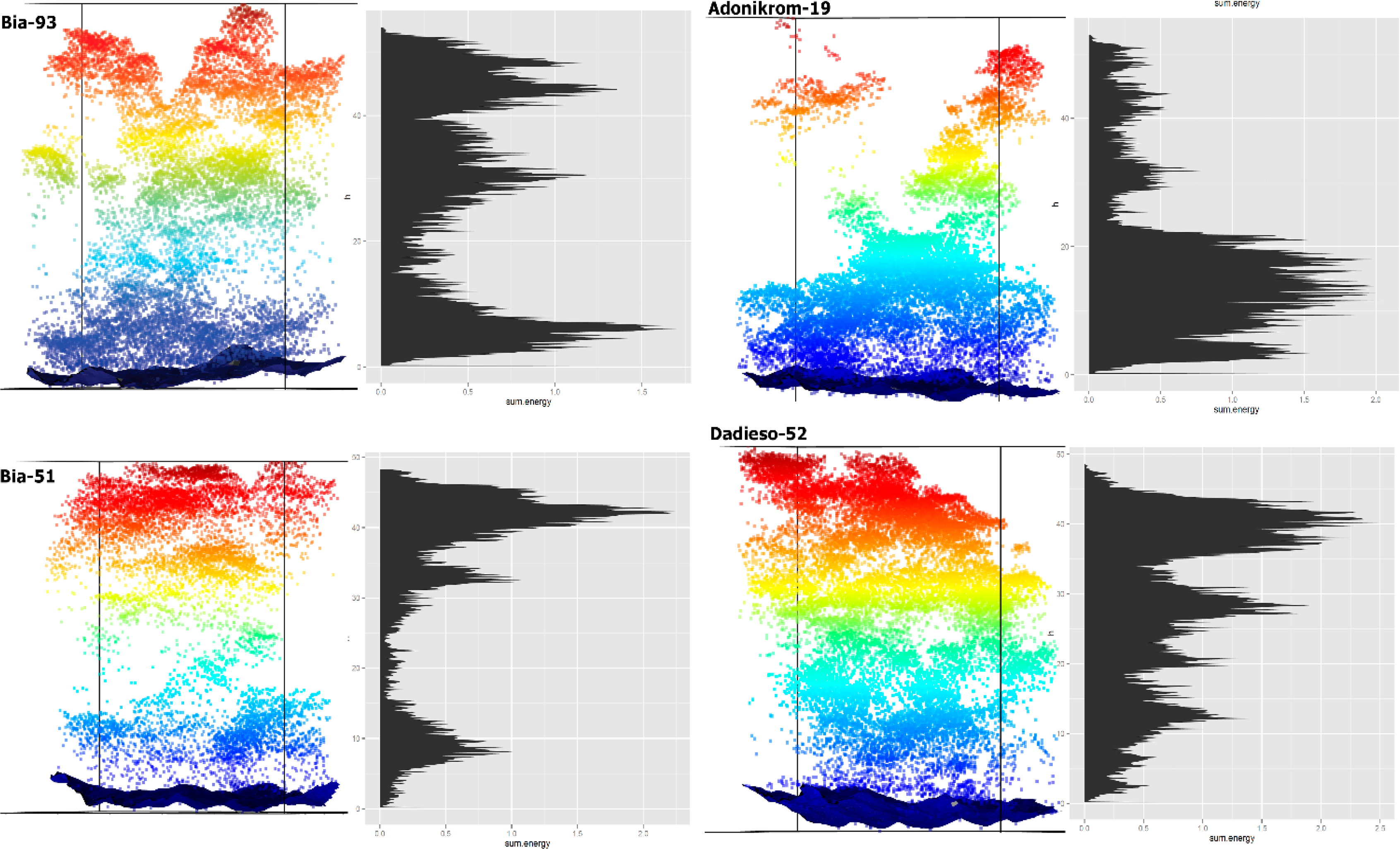
Results of investigations on large footprint LiDAR agree that biomass is significantly correlated to height-/energy-related metrics. The height of median energy (HOME) and the HOME divided by LiDAR-derived canopy height (HTRT) were found to be significant predictors of AGB in [23], considering a large area, including forest, pasture and agroforestry land. In our study case, we only have plots over forest cover, but the AGB range is comparable (∼5–200 Mg·ha⁻¹ in [23]; ∼5–500 Mg·ha⁻¹ in our case). For this reason, the next step of our method simulates HOME and HTRT at the plot level. To do so, we used the DTM extracted as described in Section 3.2.1 in Equation (3) to define height bins at regular 0.15-m intervals above the ground. The FW metric was aggregated at the bin level, which represents the return energy sampled at one-ns intervals of the full-waveform (Figure 3). In general, beam profiles are modeled by a cylindrical distribution (top-hat form) or by a 2D Gaussian distribution [36,41]; we tested both, using, for the latter case, weights relative to distance from the center of the footprint (which corresponds to the center of the plot in our simulation). This supposedly accounts for a border effect, as echoes from the canopies of trees with stems outside the plot are recorded, but ground sampling only refers to tree stems inside the plot. For this reason, we used the following Gaussian function to simulate a large footprint beam profile with a 2D Gaussian distribution:

$$w=e^{-\frac{d^2}{2{\sigma }^2}}$$

(4)

where d is the distance from the center of plot and σ is the plot diameter (40 m in our study case). Such an equation will bring a correction of 0.8 of the values at the furthest distance from the center of the plot.

All of the metrics were tested for correlation, and a selection is used for stepwise regression to determine which combination explains the highest amount of variance in our forest variables.

4. Results and Analysis

To provide a visual assessment and comparison of the results from all of the metrics tested, we graphically report in Figure 4 the coefficient of correlation (R) in a plot for each of the four aggregation operators.

p-values were always lower than 0.01 for metrics with an R-squared value higher than 0.5. The En and NoE metrics only report correlation with the median and standard deviation and not for the fifth and 95th percentile. This is because these two metrics refer to the return echoes, respectively to the distribution, in the plots, of the echo ordinal return number and of the total number of echoes. This type of metric can only take values from one to six, as six is the highest number of return echoes detected per pulse in our case study. The fifth and 95th percentile values in this case gave identical values for all plots; therefore, linear fitting was not possible.

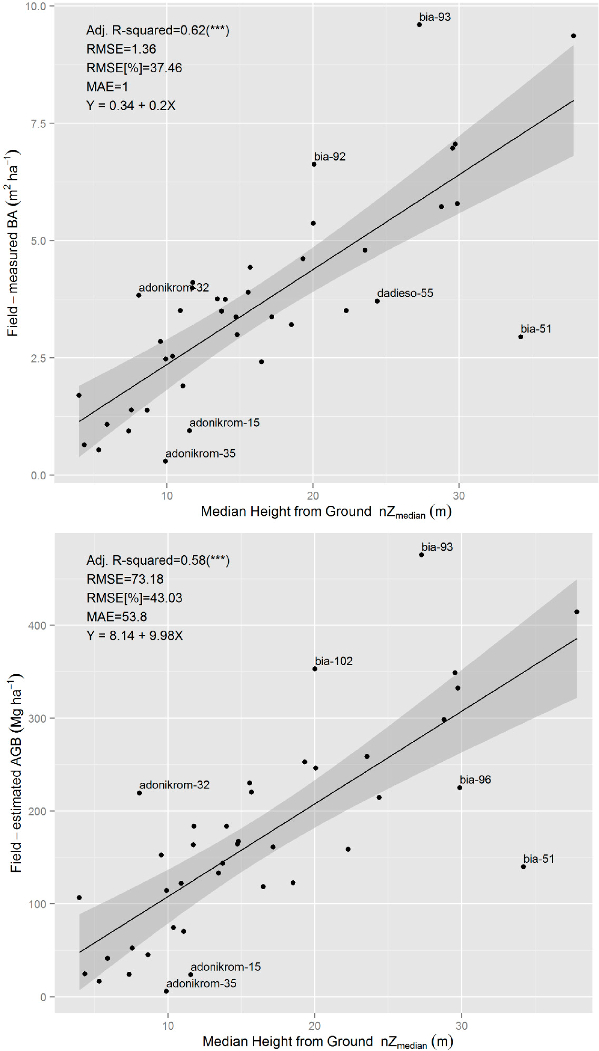
Figure 4 allows one to see the basal area and aboveground biomass degree of positive correlation with several metrics. The median value of the vertical distribution of the echoes (nZ_median) explains about 62% of the variance in the BA and 58% of the variance in the AGB; Figure 5 shows the plot of the respective linear regressions. This is slightly less in the case that the square root and the log of the two variables are considered. The total return energy (i_tot), in terms of its fifth percentile value in the plot, explains 57% and 51% of the BA and AGB, respectively. The standard deviation of the distribution of several metrics has a positive correlation with these two forest variables; the highest amount of the variance in the log-distribution of AGB (36%) is explained by the variance in the distribution of intensity for each echo.

The metrics reported in

Table 3. Selected metrics with adjusted R-squared greater than 0.55.

Dependent Variable	Predictor	Adjusted R-Squared
BA *	1 nZmedian	0.628
BA_DBH20	1 nZ median	0.617
AGB *	1 nZ median	0.577
AGB_DBH20	1 nZ median	0.568
BA_DBH20	2 i_tot5th	0.562
sqrt.BA_DBH20	2 i_tot5th	0.566

^*Represented also as plots in Figure 5.¹peak-based;²pulse-based; _DBH20 = from trees with DBH above or equal to 20 cm.

were chosen for further discussion, as they have an adjusted R-squared value above 0.55 (all p-values are lower than 0.001). Other metrics that consider the width of the signal’s peaks were found to be much less significant in describing the variables that are the object of this study.

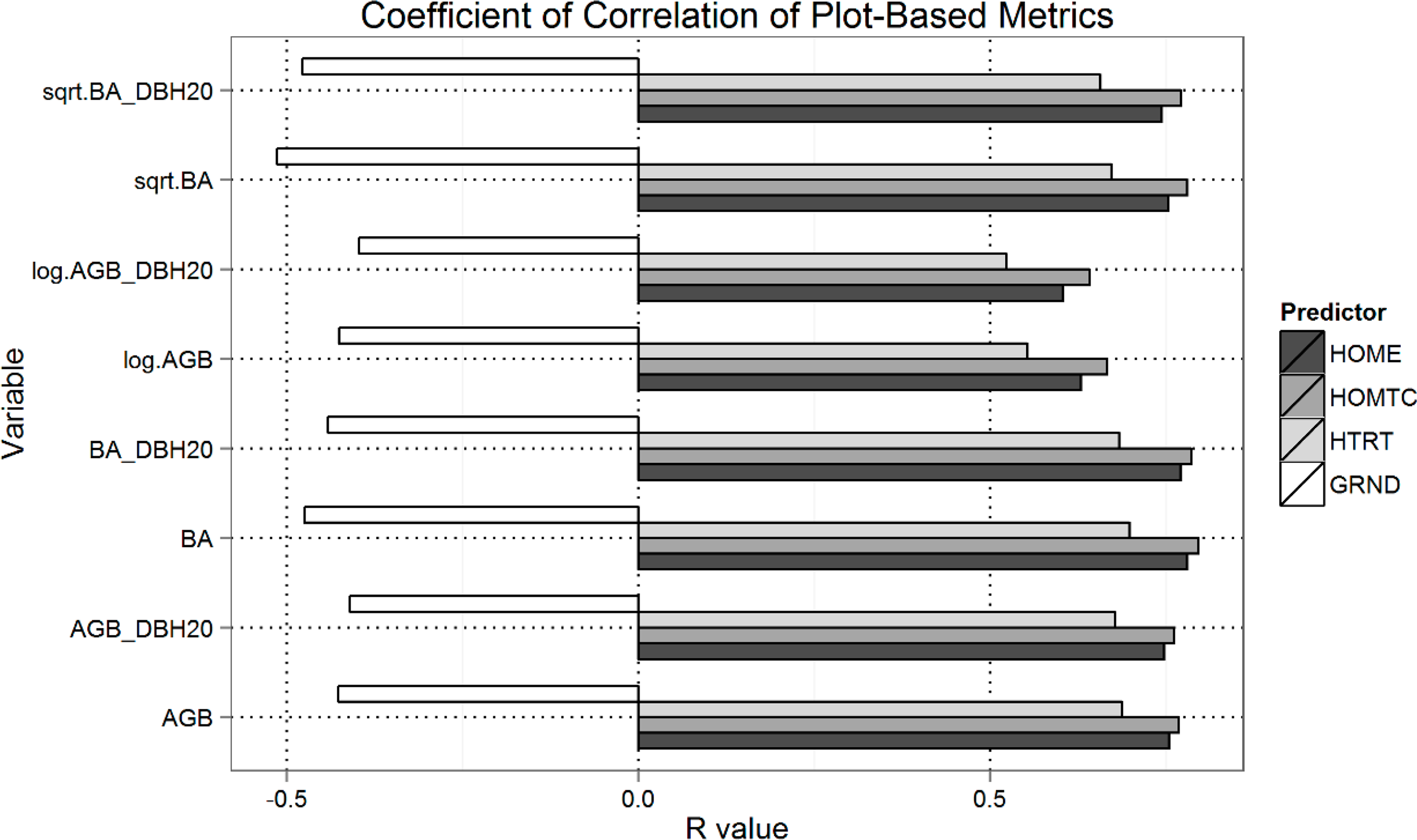
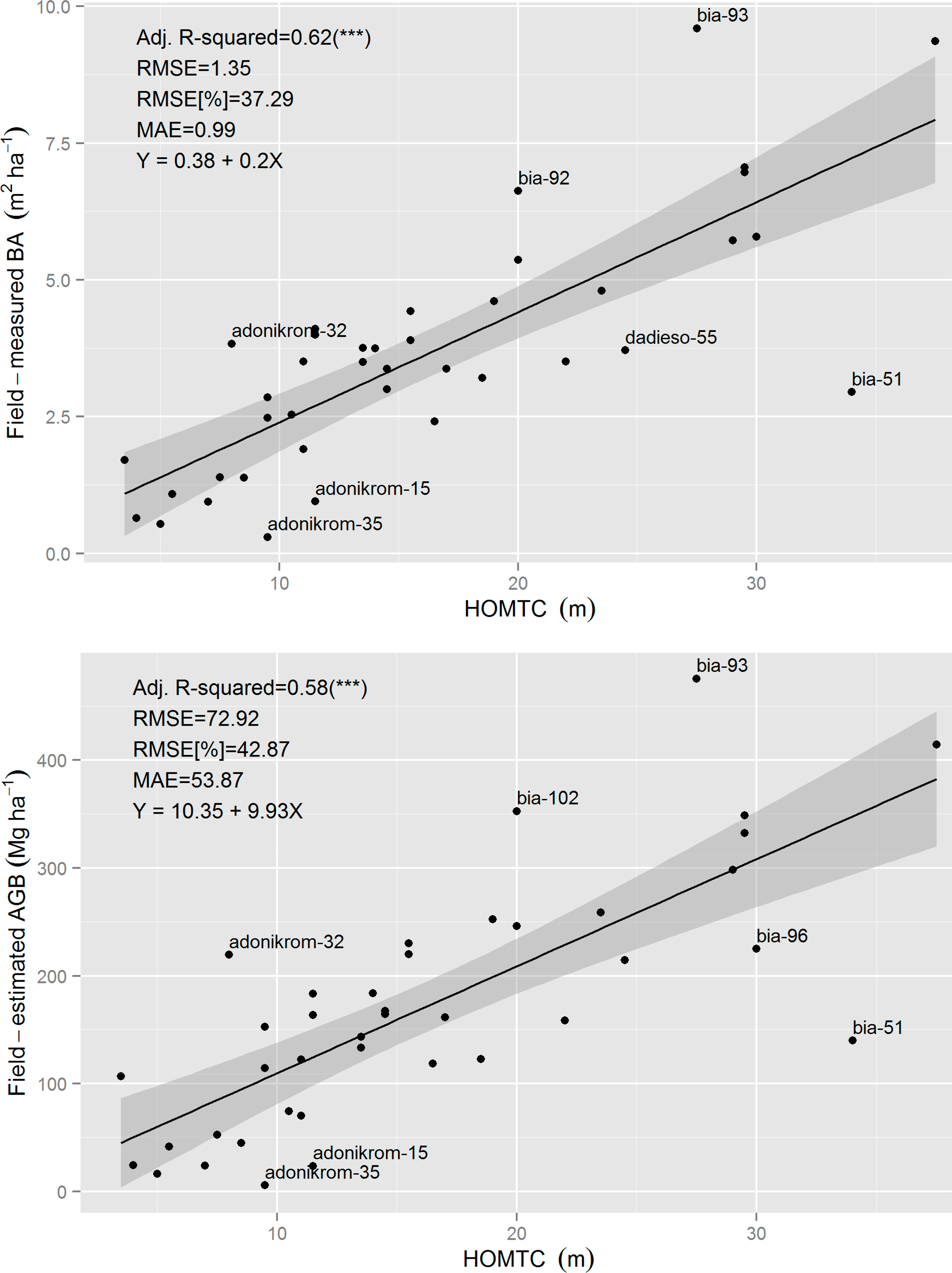
The correlation values reported as R-squared from the metrics extracted using large footprint simulation were plotted separately in Figure 6. They do not exhibit significantly different values between the different metrics, hypothetically because the vertical distribution of the echoes is the most important factor that explains the variance in the forest variables. In addition, in this case, BA and AGB have the highest values of adjusted R-squared. The overall correlation values are comparable to the best results from the metrics related to echoes and pulses reported before.

From our elaborations, we have a large set of predictors, so the number of parameters to be estimated in a regression model is definitively larger than the number of observations. Many of the former are intuitively not independent, because they represent different aspects of the same phenomenon (e.g., median value at the plot-level of peak intensities and of total intensities in the return pulse). Therefore, to select the best combination of predictors, without falling into the “trap” of over-fitting, we use Mallow’s C_p-statistic [42,43], which compares the total square of errors and the maximum R-squared; the higher the R-squared is, the better the model is, and the lower the RMSE and C_p values are, the better the model is. A complementary approach is using stepwise regression in the forward and backward directions and using Akaike’s information criterion (AIC) to determine the improvement of the model when certain predictors are added or removed. Investigations recommend replacing AIC with AICc when the sample size is small [44] and the number of parameters is large. We used both AICc and C_p, getting the same results related to which predictors are most effective and should be included in the model.

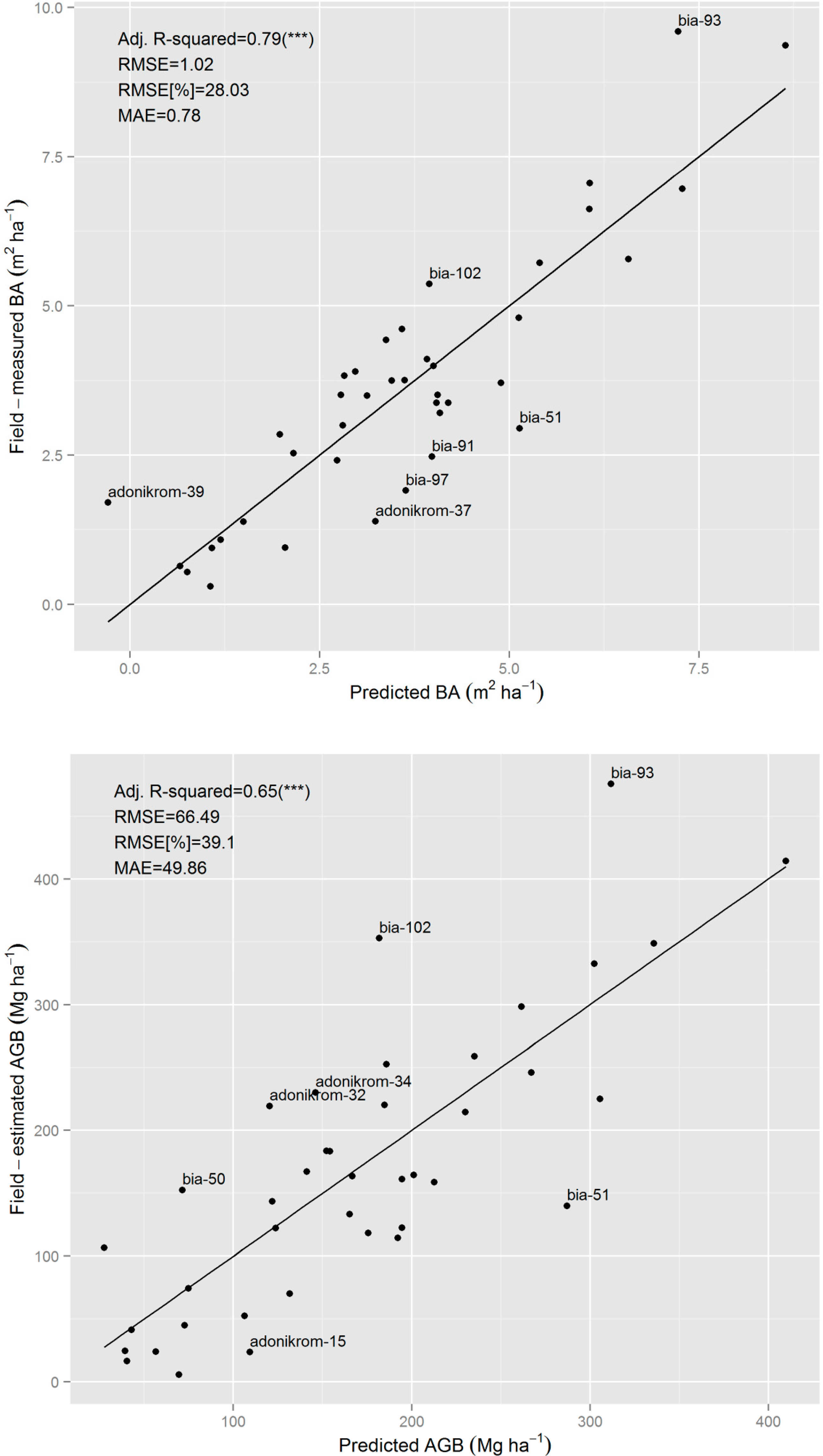
The results, reported in Figure 7, show increased values of adjusted R-squared to 79% and 65% with relative errors of 28% and 39%, respectively, for BA and AGB. The two most important factors are the distributions of nZ_median, the median of the distribution of the relative height of points from the ground plane, and i_tot, the total energy returned from the reflectors; Equations (5) and (6).

$$\begin{array}{c}\text{BA}=-10.49+0.14963\cdot {\text{nZ}}_{\text{median}}+0.01612\cdot \text{i}\_{\text{tot}}_{5\text{th}}+\\ (-0.01283)\cdot \text{i}\_{\text{tot}}_{\text{median}}+0.01972\cdot \text{i}\_{\text{tot}}_{\text{stdDev}}\end{array}$$

(5)

$$\text{AGB}=-362.06+7.611\cdot {\text{nZ}}_{\text{median}}+0.117\cdot \text{i}\_{\text{tot}}_{5\text{th}}$$

(6)

The leave-one-out cross-validation (looCV) method was used to assess the prediction accuracy of three models: (i) nZ_median only; (ii) the model chosen with stepwise regression shown in Equation (5) above; and (iii) the HOME-nZ metric from large footprint simulation, as it gave the best result against AGB, as can be inferred from Figure 6. In turn, for each of the forty observations (plots), a single observation from the original sample was selected as validation data and the remaining as training data. The accuracy was computed as the absolute RMSE, the BIAS and the relative RMSE (%), as in the equations below:

$${\mathit{RMSE}}_{\mathit{looCV}}=\sqrt{\frac{1}{n}\sum _{i=1}^n{\left(x-\widehat{x}\right)}^2}$$

(7)

$${\mathit{BIAS}}_{\mathit{looCV}}=\frac{1}{n}\sum _{i=1}^n(x-\widehat{x})$$

(8)

$${\mathit{RMSE}}_{\mathit{looCV}}(\%)=100\times {\mathit{RMSE}}_{\mathit{looCV}}\overline{x}$$

(9)

where n is the number of observations, x is the observed value and x̂ is the predicted value from the looCV procedure; x̄ is the average of the observed values. The results are reported in

Table 4. The accuracy of prediction in the models for the estimation of AGB and BA. Both regression equations use both the peak-based metric (nZ) and pulse-based metric (i_tot).

	Adj-R2	a MAE	a RMSElooCV	a BIASlooCV	RMSElooCV (%)
1 BA ∼ nZmedian	0.62	1.0	1.14	0.37	37%
2 BA ∼ HOMTC	0.62	0.99	1.42	0.38	39%
3 BA ∼ Equation 5	0.79	0.78	1.14	−0.04	29%
1 AGB ∼ nZmedian	0.58	53.80	76.7	9.45	45%
2 AGB ∼ HOMTC	0.58	53.87	76.4	10.35	45%
3 AGB ∼ Equation (6)	0.65	49.86	68.2	0	40%

^aRespectively, m²·ha⁻¹ for basal area and Mg·ha⁻¹ for aboveground biomass;¹Figure 5;²Figure 7;³Figure 8.

along with the adjusted R-squared value of each fitted model.

5. Discussion

The results from the different combinations of metrics are in agreement with other studies that use LiDAR-derived metrics for assessing estimation models of AGB and BA over tropical forests. The models at the plot-scale in [23] show similar values of dispersion in the non-asymptotic relationships found by stepwise regression. Furthermore, in [6] and [45], where a broader state of the art is presented, reported results show that LiDAR estimation of biomass reaches higher values of the coefficient of determination (∼0.8–0.9 and above) in conifer forests [46], whereas hardwood tests generally reach lower values and depend on the complexity of the forest structure, both in the vertical and in the horizontal directions.

The aim of the paper was to provide insights into how metrics from LiDAR, both regarding return echoes (peaks), the complete return pulse signal and aggregated metrics at the plot level, simulate a large footprint return. The relationship between the two best metrics (see Equation (5)) and the high correlation with the large footprint metrics show that the vertical distribution of the vegetation is of great importance.

The median height of the echoes above the ground surface (nZ) alone is enough to explain quite a bit of variance in the biomass (58%). The other percentiles of this metric have a lower degree of correlation, but are still significant. The 95th percentile of nZ has a higher correlation with the log-normal distribution of AGB than with the linear distribution of AGB, whereas the opposite is true for the median of nZ. This may be due to the fact that the AGB distribution is skewed to the left (lower values are more frequent) than the distribution of the predictor (i.e., the nZ metric). This implies that plots with taller trees, which weigh more in the 95th percentile of the nZ metric, are better described when their AGB is log-transformed. Therefore, their corresponding plots against the log-transformed AGB values, on the right side, increase the R-squared values for the former and lower it for the latter metric. The distribution of total return energy (i_tot) can describe a high amount of variance (57%) of BA of trees with its fifth percentile metric. As can be inferred from Figure 4, there is no significant difference between linear BA values nor those transformed by their square root, nor between all trees measured and only trees with a DBH above 0.2 m. In Table 3, we do not report the R-squared values for all results of i_tot_5th with BA, because they are borderline within the 0.55 value threshold with the ones not shown falling just below that value. Another note regarding this metric is that it shows the same type of correlation values for all three percentiles, i.e., 5th, 50th (median) and 95th percentile, whereas there is no significant correlation (∼0.2 R-squared) between its standard deviation and the forest variables. A more detailed view on the results of the adjusted R-squared values of i_tot is shown in

Table 5. The i_tot pulse-based metric and its R-squared values, from linear fitting AGB and BA variables, in descending order. _DBH20 = trees with a DBH equal to or above 20 cm.

Variable	Predictor	Adj. R-Squared
BA_DBH20	i_tot5th	0.56
BA	i_tot5th	0.55
BA_DBH20	i_totmedian	0.51
BA	i_totmedian	0.49
BA_DBH20	i_tot95th	0.48
BA	i_tot95th	0.45
AGB_DBH20	i_tot5th	0.44
AGB	i_tot5th	0.43
AGB_DBH20	i_totmedian	0.40
AGB	i_totmedian	0.39
AGB_DBH20	i_tot95th	0.36
AGB	i_tot95th	0.34

, where two relationships are clear: (i) the basal area is better predicted than aboveground biomass; and (ii) trees with a diameter at breast height equal to or above 20 cm are better predicted, as well. The fifth percentile in both cases leads to better results, and this might be explained by examining its definition: the value below which 5% of the observations of intensity values are found. This value, from our results, has a direct relationship with AGB and BA and is more sensible than higher percentiles. This can be explained by the fact that there are fewer low intensity values (negative skewed uni-modal frequency distribution) in plots with more BA and AGB. These observations may lead one to consider that the total intensity recorded by the digitizer in each plot is well related to the amount of reflectors and their capability of reflecting the laser beam energy.

Leaves are better reflectors than other elements in forests (branches, stems or ground), particularly so in broadleaves [24], thus returning stronger intensity returns. The amount of intercepted laser energy by foliage is correlated to the well-known indices related to leaf area (e.g., leaf area index, LAI) which is, in turn, related to stem diameter by different allometric relationships [47,48], as was also tested on large footprint FW LiDAR in [49]. Intensity was also found to give a valid contribution to vegetation cover classification in [50] due to the above reasons. These points contribute to explaining the positive correlation between the total return intensity and the measured AGB and BA values.

A reason for the high error in estimating AGB for some plots may be the limitation of the median values of a distribution to describe the actual vertical structure of the forest. Figure 3 shows four profiles of echoes from respective plots chosen with the purpose of showing two plots with higher error represented on the left (Bia-93 and Bia-51) and two other plots with low error on the right (Adonikon-19 and Dadieso-52), the latter, respectively, with lower and higher aboveground biomass values. If we analyze the outliers considering Figure 3, the profiles show that bimodal distributions may be related to the high errors in these two cases. The median and other frequency metrics can have similar values in these two different cases. If this is the case, improvements may result from applying a weighting function related to height above ground, as was adopted in [18]. In that study case, the authors apply what they call K-functions, which return different values depending on height fraction K(h). The values of K(h) were found using training datasets and fitting a linear functional model. This approach has not been used, because the number of plots are not so numerous to allow extracting a significant number of training areas for such a method.

Considering the top left plot in Figure 4, it is evident that the variability (standard deviation) of some predictors is also related to biomass and basal area. In this case, the R-squared values are all below 0.5, but it is still interesting to analyze the metric that has the highest correlation values, the last echo energy (LE) metric. This metric represents the distribution of the intensities from the last pulses, so a high variance implies a high variance invariance in reflective surfaces’ distribution and the gap fraction in the canopy. An opposite scenario, with low variance in those two structural characteristics, would be related to even-aged forests with a single canopy layer and an overall lower biomass. The LE standard deviation is a better predictor than the other metrics, probably because it carries the variability of multiple return echoes. A higher number of returns will give lower LE values compared to less echoes or single echoes. This way, the variance in the distribution in a plot of this metric is related both to canopy density (gaps) and to vertical variability, which reflects biomass content.

Pulse metrics are particularly interesting, because they imply the use of the whole return FW and do not require the peak detection step, which is time consuming and implies more or less sophisticated steps. From all of the metrics of this category, only the total return intensity (i_tot) had a high R-squared value, as discussed previously. This supports the importance of the vertical distribution of the LiDAR return segments, which cannot be substituted with metrics from pulses only. One scenario can be the usage of the i_tot metric to have the first estimate of AGB before proceeding with the complete FW processing in a stratified approach, for example, to continue further estimations with peak metrics in areas above a specific value of estimated AGB.

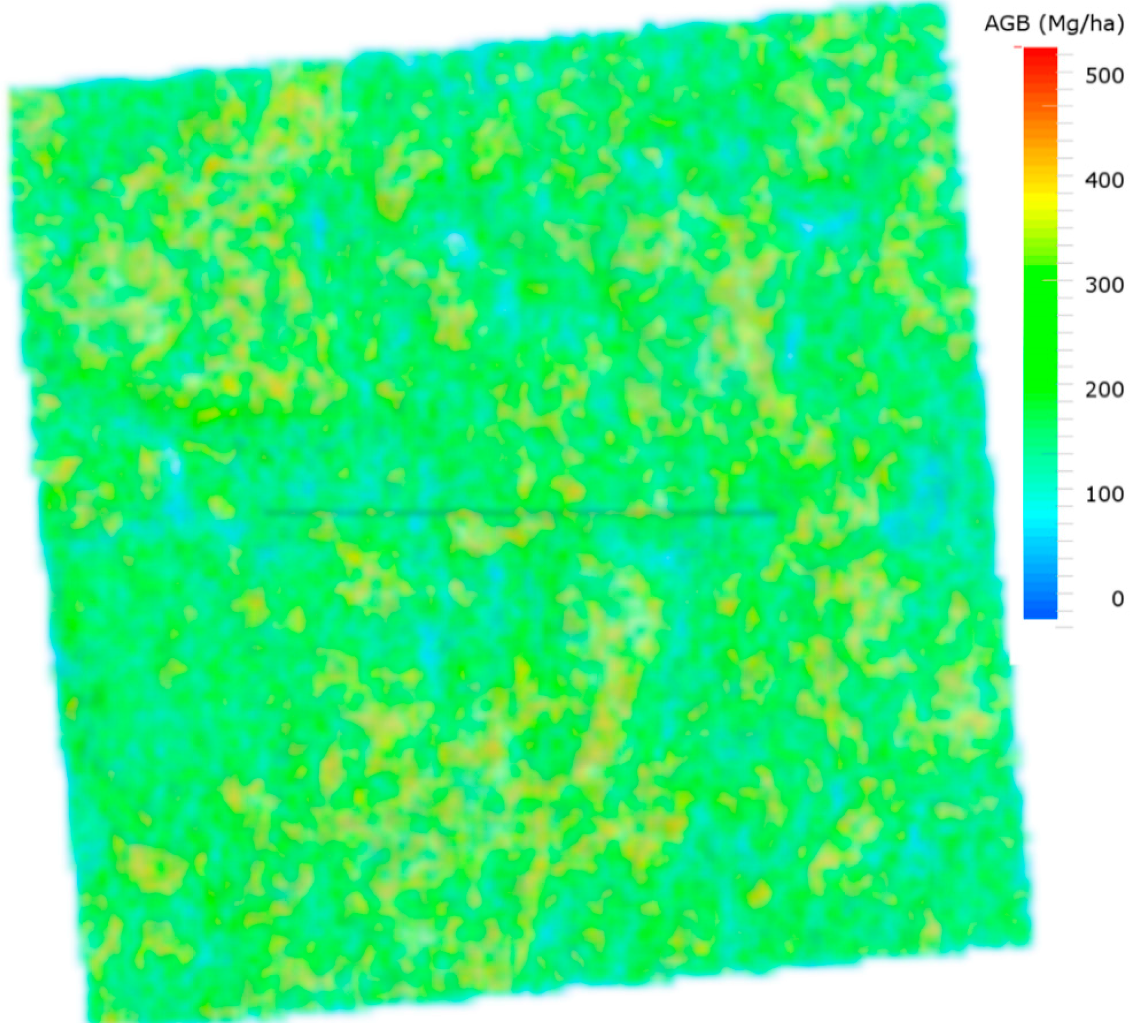
The results from the large footprint simulation do not show significant differences between the different metrics, as can be seen in Figure 6. The cross-validation results show that even if the R-squared values prove a significant correlation with AGB and BA observations in plots, the absolute and relative RMSE_looCV values are high, showing that the model is not robust in this context of the high range and variability of AGB and BA values. As discussed previously, a weighting function also in this case may prove to be a solution. Care must be taken to apply such functions though, because these might lead to case-specific models, which have a low power of generalization, thus eliminating the value of the model per se. Earlier work by other authors has shown the validity of using height distribution metrics from LiDAR for estimating biomass or volume [18,51–54], leading to site-specific models. The result of the overall best model for explaining AGB, with adjusted R-squared equal to 0.65, is also similar to other experiences in similar conditions and with similar datasets [21]. Figure 9 shows a raster representation of estimations at the pixel level with 2 m × 2-m resolution. We tried to explain AGB and BA variances with a general model and had less accurate results. Nevertheless, the results can be considered as positive, bearing in mind the wide range of AGB values, from ∼5 Mg·ha⁻¹ to ∼500 Mg·ha⁻¹, and the high variability (the standard deviation of AGB is 127 Mg·ha⁻¹ over a mean of 170 Mg·ha⁻¹).

6. Conclusions

The spatial distribution of aboveground biomass and basal area are fundamental information in forestry. In our study case, we consider tropical forests with values of AGB covering a wide range of values, from ∼5 Mg·ha⁻¹ to ∼500 Mg·ha⁻¹. Regarding BA, we obtain 79% of variance explained with an RMSE of ∼1.14 m² (∼29%) using cross-validation with the leave-one-out technique. AGB variance is explained at its best at 65% by a model with two metrics of variance with an RMSE of ∼68 Mg·ha⁻¹ (∼40%). The vertical distribution of echoes was the most important information in the models in terms of the median of the values in each plot. The information on intensity (i_tot) in the form of normalized return energy recorded by the digitizer contributes very significantly in terms of its fifth percentile, its median and also its standard deviation. More sophisticated metrics derived from FW width in this scenario also provide significant correlations with AGB and BA, but do not bring significant benefit with respect to the abovementioned predictors. Aggregating vertically the data simulating large footprints brings positive results, with high correlations, but this does not improve the results to such a degree that this type of procedure can be deemed better than analyzing plot-level metrics. Both 3D position and intensity information, which our work concludes to be the most important factors, is present in DR data, but no control over the online processing step, which provides this data automatically on-board the aircraft, is possible. FW data allows improved control over the intensity calibration and peak detection accuracy, and this investigation proves that efforts in this direction, past and future, will be rewarded by improving the accuracy in predicting forest variables in complex ecosystems, such as tropical rain forests. The intensity information in this study refers to the total return intensity of the pulse; thus, it can potentially be used directly from FW data without the peak detection step for an initial rough estimation of biomass across the area of interest.

Further research is required to assess the efficacy of our methods across varying landscapes and biomes. The validation of our approach was supported by having ground-truth samples, which are not easily obtainable in such conditions. The increase in the use of airborne and spaceborne LiDAR data is another factor, which contributes towards making this study significant.

The vertical distribution of return echoes and the distribution of the total return energy is related to AGB and BA at the plot level. While the former requires processing the FW to extract echoes and, thus, their position in three-dimensional space, the latter can be applied using a simpler and more direct method.

The potential of retrieving these observations from space is a tangible possibility with the planned future missions from Earth-observing satellites, e.g., DESDynI [55]. The positive results in this study of estimating AGB and BA using both plot-level information and simulated large footprint FW data adds significant confirmation to other investigations that point to the success of LiDAR data towards monitoring forest resources from space-borne sensors.

References

- Ussyshkin, V.; Theriault, L. Airborne Lidar: Advances in discrete return technology for 3D vegetation mapping. Remote Sens 2011, 3, 416–434. [Google Scholar]
- Toth, C.; Laky, S.; Zaletnyik, P.; Grejner-Brzezinska, D. Peak detection from full-waveform data. Proceedings of International LiDAR Mapping Forum (ILMF 2011), New Orleans, LA, USA, 7–9 February 2011.
- Reitberger, J.; Krzystek, P.; Stilla, U. Analysis of full waveform LiDAR data for the classification of deciduous and coniferous trees. Int. J. Remote Sens 2008, 29, 1407–1431. [Google Scholar]
- Pirotti, F.; Grigolato, S.; Lingua, E.; Sitzia, T.; Tarolli, P. Laser scanner applications in forest and environmental sciences. Ital. J. Remote Sens 2012, 44, 109–123. [Google Scholar]
- Chave, J.; Condit, R.; Aguilar, S.; Hernandez, A.; Lao, S.; Perez, R. Error propagation and scaling for tropical forest biomass estimates. Philos. Trans. R. Soc. Lond. B. Biol. Sci 2004, 359, 409–420. [Google Scholar]
- Koch, B. Status and future of laser scanning, synthetic aperture radar and hyperspectral remote sensing data for forest biomass assessment. ISPRS J. Photogramm. Remote Sens 2010, 65, 581–590. [Google Scholar]
- Lefsky, M.A.; Harding, D.J.; Keller, M.; Cohen, W.B.; Carabajal, C.C.; del Bom Espirito-Santo, F.; Hunter, M.O.; de Oliveira, R. Estimates of forest canopy height and aboveground biomass using ICESat. Geophys. Res. Lett 2005, 32, L22S02. [Google Scholar]
- Yáñez, L.; Homolová, L.; Malenovský, Z.; Schaepman, M. Geometrical and structural parametrisation of forest canopy radiative transfer by measurements. Int. Arch. Photogramm. Remote Sens. Spat. Inf. Sci 2008, 37, 45–50. [Google Scholar]
- Saatchi, S.S.; Harris, N.L.; Brown, S.; Lefsky, M.; Mitchard, E.T.A.; Salas, W.; Zutta, B.R.; Buermann, W.; Lewis, S.L.; Hagen, S.; et al. Benchmark map of forest carbon stocks in tropical regions across three continents. Proc. Natl. Acad. Sci. USA 2011, 108, 9899–9904. [Google Scholar]
- Baccini, A.; Goetz, S.J.; Walker, W.S.; Laporte, N.T.; Sun, M.; Sulla-Menashe, D.; Hackler, J.; Beck, P.S.A.; Dubayah, R.; Friedl, M.A.; et al. Estimated carbon dioxide emissions from tropical deforestation improved by carbon-density maps. Nat. Clim. Chang 2012, 2, 182–185. [Google Scholar]
- Cutler, M.E.J.; Boyd, D.S.; Foody, G.M.; Vetrivel, A. Estimating tropical forest biomass with a combination of SAR image texture and Landsat TM data: An assessment of predictions between regions. ISPRS J. Photogramm. Remote Sens 2012, 70, 66–77. [Google Scholar]
- Hill, T.C.; Williams, M.; Bloom, A.A.; Mitchard, E.T.A.; Ryan, C.M. Are inventory based and remotely sensed above-ground biomass estimates consistent? PLoS One 2013, 8, e74170. [Google Scholar]
- Foody, G.M.; Curran, P.J. Estimation of tropical forest extent and regenerative stage using remotely sensed data. J. Biogeogr 1994, 21, 223–244. [Google Scholar]
- Vaglio Laurin, G.; Chen, Q.; Lindsell, J.A.; Coomes, D.A.; Frate, F.D.; Guerriero, L.; Pirotti, F.; Valentini, R. Above ground biomass estimation in an African tropical forest with lidar and hyperspectral data. ISPRS J. Photogramm. Remote Sens 2014, 89, 49–58. [Google Scholar]
- Tonolli, S.; Dalponte, M.; Vescovo, L.; Rodeghiero, M.; Bruzzone, L.; Gianelle, D. Mapping and modeling forest tree volume using forest inventory and airborne laser scanning. Eur. J. For. Res 2010, 130, 569–577. [Google Scholar]
- Nelson, R. Separating the ground and airborne laser sampling phases to estimate tropical forest basal area, volume, and biomass. Remote Sens. Environ 1997, 60, 311–326. [Google Scholar]
- Gobakken, T.; Næsset, E.; Nelson, R.; Martin, O.; Gregoire, T.G.; Ståhl, G.; Holm, S.; Ole, H.; Astrup, R. Estimating biomass in Hedmark County, Norway using national forest inventory field plots and airborne laser scanning. Remote Sens. Environ 2012, 123, 443–456. [Google Scholar]
- Zhao, K.; Popescu, S.; Nelson, R. Remote sensing of environment lidar remote sensing of forest biomass : A scale-invariant estimation approach using airborne lasers. Remote Sens. Environ 2009, 113, 182–196. [Google Scholar]
- Naesset, E.; Bollandsas, O.M.; Gobakken, T. Comparing regression methods in estimation of biophysical properties of forest stands from two different inventories using laser scanner data. 2005, 94, 541–553. [Google Scholar]
- Bortolot, Z.J.; Wynne, R.H. Estimating forest biomass using small footprint LiDAR data: An individual tree-based approach that incorporates training data. ISPRS J. Photogramm. Remote Sens 2005, 59, 342–360. [Google Scholar]
- Boudreau, J.; Nelson, R.; Margolis, H.; Beauduin, A.; Guindon, L.; Kimes, D. Regional aboveground forest biomass using airborne and spaceborne LiDAR in Québec. Remote Sens. Environ 2008, 112, 3876–3890. [Google Scholar]
- Ni, X.; Park, T.; Choi, S.; Shi, Y.; Cao, C.; Wang, X.; Lefsky, M.; Simard, M.; Myneni, R. Allometric scaling and resource limitations model of tree heights: Part 3. Model optimization and testing over continental China. Remote Sens 2014, 6, 3533–3553. [Google Scholar]
- Drake, J.B.; Dubayah, R.O.; Clark, D.B.; Knox, R.G.; Blair, J.B.; Hofton, M.A.; Chazdon, R.L.; Weishampel, J.F.; Prince, S. Estimation of tropical forest structural characteristics using large-footprint lidar. Remote Sens. Environ 2002, 79, 305–319. [Google Scholar]
- Adams, T.; Beets, P.; Parrish, C. Extracting more data from LiDAR in forested areas by analyzing waveform shape. Remote Sens 2012, 4, 682–702. [Google Scholar]
- Neuenschwander, A.L. Landcover classification of small-footprint, full-waveform lidar data. J. Appl. Remote Sens 2009, 3, 033544. [Google Scholar]
- Pirotti, F. Analysis of full-waveform LiDAR data for forestry applications: A review of investigations and methods. iForest-Biogeosci. For 2011, 4, 100–106. [Google Scholar]
- Hyyppä, J.; Holopainen, M.; Olsson, H. Laser scanning in forests. Remote Sens 2012, 4, 2919–2922. [Google Scholar]
- Hall, J.B.; Swaine, M.D. Distribution and Ecology of Vascular Plants in a Tropical Rain Forest; Springer: Dordrecht, The Netherlands, 1981. [Google Scholar]
- El-Rabbany, A. Engineer’s Guide to GPS; Artech House: London, UK, 2002; p. 216. [Google Scholar]
- Pirotti, F.; Guarnieri, A.; Vettore, A. Analysis of correlation between full-waveform metrics, scan geometry and land-cover: An application over forests. ISPRS Ann. Photogramm. Remote Sens. Spat. Inf. Sci 2013, II-5/W2, 235–240. [Google Scholar]
- Pirotti, F.; Guarnieri, A.; Masiero, A.; Vettore, A.; Lingua, E. Processing lidar waveform data for 3D visual assessment of forest environments. Int. Arch. Photogramm. Remote Sens. Spat. Inf. Sci 2014, XL-5, 493–499. [Google Scholar]
- Parrish, C.E. Vertical Object Extraction from Full-Waveform Lidar Data Using a 3D Wavelet-Based Approach; The University of Wisconsin-Madison: Madison, WI, USA, 2007. [Google Scholar]
- Roncat, A.; Wieser, M.; Briese, C.; Bollmann, E.; Sailer, R.; Klug, C.; Pfeifer, N. Analysing the suitability of radiometrically calibrated full-waveform lidar data for delineating Alpine rock glaciers. ISPRS Ann. Photogramm. Remote Sens. Spat. Inf. Sci 2013, II-5/W2, 247–252. [Google Scholar]
- Billauer, E. Peakdet: Peak Detection Using MATLAB. Available online: http://www.billauer.co.il/peakdet.html (accessed on 12 March 2014).
- Wagner, W. Radiometric calibration of small-footprint full-waveform airborne laser scanner measurements: Basic physical concepts. ISPRS J. Photogramm. Remote Sens 2010, 65, 505–513. [Google Scholar]
- Stilla, U.; Jutzi, B. Waveform analysis for small-footprint pulsed laser systems. In Topographic Laser Ranging and Scanning: Principles and Processing; Shan, J., Toth, C.K., Eds.; CRC Press: Boca Raton, FL, USA, 2009; pp. 215–234. [Google Scholar]
- Wagner, W.; Ullrich, A.; Ducic, V.; Melzer, T.; Studnicka, N. Gaussian decomposition and calibration of a novel small-footprint full-waveform digitising airborne laser scanner. ISPRS J. Photogramm. Remote Sens 2006, 60, 100–112. [Google Scholar]
- Pirotti, F.; Guarnieri, A.; Vettore, A. Vegetation filtering of waveform terrestrial laser scanner data for DTM production. Appl. Geomat 2013, 5, 311–322. [Google Scholar]
- Pirotti, F.; Guarnieri, A.; Vettore, A. Ground filtering and vegetation mapping using multi-return terrestrial laser scanning. ISPRS J. Photogramm. Remote Sens 2013, 76, 56–63. [Google Scholar]
- Zhang, K.; Chen, S.; Whitman, D.; Shyu, M.; Yan, J.; Zhang, C. A progressive morphological filter for removing nonground measurements from airborne LiDAR data. IEEE Trans. Geosci. Remote Sens 2003, 41, 872–882. [Google Scholar]
- Kamermann, G.W. Laser radar. In Active Electro-Optical Systems, The Infrared & Electro-Optical Systems Handbook; Fox, C.S., Ed.; SPIE Optical Engineering Press: Dallas, TX, USA, 1993. [Google Scholar]
- Mallows, C.L. Some comments onCp. Technometrics 1973, 15, 661. [Google Scholar]
- Gilmour, S.G. The interpretation of Mallows’s Cp-Statistic. J. R. Stat. Soc 1996, 45, 49–56. [Google Scholar]
- Burnham, K.P.; Anderson, D.R. Multimodel inference: Understanding AIC and BIC in model selection. Sociol. Methods Res 2004, 33, 261–304. [Google Scholar]
- Lim, K.; Treitz, P.; Wulder, M.; St-Onge, B.; Flood, M. LiDAR remote sensing of forest structure. Prog. Phys. Geogr 2003, 27, 88–106. [Google Scholar]
- Nelson, R.; Short, A.; Valenti, M. Measuring biomass and carbon in Delaware using an airborne profiling lidar. Proceedings of Scandlaser Scientific Workshop on Aiborne Laser Scanning of Forests, Umeå, Sweden, 3–4 September 2003; Hyyppä, J., Næsset, E., Olsson, H., Eds.; pp. 134–144.
- Calvo-Alvarado, J.C.; McDowell, N.G.; Waring, R.H. Allometric relationships predicting foliar biomass and leaf area: Sapwood area ratio from tree height in five Costa Rican rain forest species. Tree Physiol 2008, 28, 1601–1608. [Google Scholar]
- McWilliam, A.-L.C.; Roberts, J.M.; Cabral, O.M.R.; Leitao, M.V.B.R.; de Costa, A.C.L.; Maitelli, G.T.; Zamparoni, C.A.G.P. Leaf area index and above-ground biomass of terra firme rain forest and adjacent clearings in Amazonia. Funct. Ecol 1993, 7, 310. [Google Scholar]
- Lefsky, M.A.; Harding, D.; Cohen, W.; Parker, G.; Shugart, H. Surface lidar remote sensing of basal area and biomass in deciduous forests of eastern Maryland, USA. Remote Sens. Environ 1999, 67, 83–98. [Google Scholar]
- Schreier, H.; Lougheed, J.; Tucker, C.; Leckie, D. Automated measurements of terrain reflection and height variations using an airborne infrared laser system. Int. J. Remote Sens 1985, 6, 101–113. [Google Scholar]
- Drake, J.B.; Knox, R.G.; Dubayah, R.O.; Clark, D.B.; Condit, R.; Blair, J.B.; Hofton, M. Above-ground biomass estimation in closed canopy neotropical forests using lidar remote sensing: Factors. Glob. Ecol. Biogeogr 2003, 12, 147–159. [Google Scholar]
- Means, J.E.; Acker, S.A.; Fitt, B.J.; Renslow, M.; Emerson, L.; Hendrix, C.J. Predicting forest stand characteristics with airborne scanning lidar. Photogramm. Eng. Remote Sens 2000, 66, 1367–1371. [Google Scholar]
- Næsset, E. Predicting forest stand characteristics with airborne scanning laser using a practical two-stage procedure and field data. Remote Sens. Environ 2002, 80, 88–99. [Google Scholar]
- Straub, C.; Koch, B. Enhancement of bioenergy estimations within forests using airborne laser scanning and multispectral line scanner data. Biomass Bioenergy 2011, 35, 3561–3574. [Google Scholar]
- DESDynI Overview. Available online: http://decadal.gsfc.nasa.gov/documents/06_DESDynI.pdf (accessed on 12 March 2014).