Assessment of Total Suspended Sediment Distribution under Varying Tidal Conditions in Deep Bay: Initial Results from HJ-1A/1B Satellite CCD Images

Abstract
: Using Deep Bay in China as an example, an effective method for the retrieval of total suspended sediment (TSS) concentration using HJ-1A/1B satellite images is proposed. The factors driving the variation of the TSS spatial distribution are also discussed. Two field surveys, conducted on August 29 and October 26, 2012, showed that there was a strong linear relationship (R2 = 0.9623) between field-surveyed OBS (optical backscatter) measurements (5-31NTU) and laboratory-analyzed TSS concentrations (9.89–35.58 mg/L). The COST image-based atmospheric correction procedure and the pseudo-invariant features (PIF) method were combined to remove the atmospheric effects from the total radiance measurements obtained with different CCDs onboard the HJ-1A/1B satellites. Then, a simple and practical retrieval model was established based on the relationship between the satellite-corrected reflectance band ratio of band 3 and band 2 (Rrs3/Rrs2) and in-situ TSS measurements. The R2 of the regression relationship was 0.807, and the mean relative error (MRE) was 12.78%, as determined through in-situ data validation. Finally, the influences of tide cycles, wind factors (direction and speed) and other factors on the variation of the TSS spatial pattern observed from HJ-1A/1B satellite images from September through November of 2008 are discussed. The results show that HJ-1A/1B satellite CCD images can be used to estimate TSS concentrations under different tides in the study area over synoptic scales without using simultaneous in-situ atmospheric parameters and spectrum data. These findings provide strong informational support for numerical simulation studies on the combined influence of tide cycles and other associated hydrologic elements in Deep Bay.1. Introduction
Inland and estuarine coastal waters that are closely associated with human activities face serious pollution and eutrophication problems. For example, since the late 1990s, the number, size and diversity of toxic algal blooms have increased substantially in China’s inland and coastal waters [1,2]. From May to June 2007, an algal bloom caused a water supply crisis in Wuxi City, forcing the closure of the waterworks and affecting nearly 1,000,000 people [3]. Eutrophication, indicated by phytoplankton blooms in the upper reaches of the estuary in recent years, has induced frequent algal blooms and red tides in the coastal waters of Guangdong and Hong Kong [4]. There are also several reports of algal blooms and red tides in Deep Bay [5]. Therefore, it is important to monitor water quality effectively and to understand how the health of the marine environment is influenced by multifarious natural and anthropogenic factors [6,7].
Total suspended sediment (TSS) is one of the major factors that affect the penetration of light into water and, as a result, the primary production of coastal waters, especially in bays or estuaries. High concentrations of TSS directly affect water quality and benthic materials. The influence of sediment on a marine ecosystem can be permanent and potentially detrimental in many cases. Traditional field sampling methods are often insufficient in terms of spatial and temporal coverage to derive statistically meaningful results [8]. Satellite remote sensing, theoretically allowing the collection of water quality data over a large area simultaneously, may be a promising way to provide improved coverage for water management authorities if effective methods are applied [9,10].
There have been many successful cases in which the TSS of turbid waters has been retrieved from satellite sensor data in the past 40 years [6–19]. In the 1970s, just after the successful launch of Landsat-1, researchers built a quantitative statistical model for suspended sediment retrieval using multispectral scanner (MSS) remotely sensed images [13]. Subsequently, MODIS, MERIS, SPOT and Landsat TM/ETM+ have been used to assess the TSS concentration in different study areas [8,10–21].
However, there has been no attempt to monitor water constituents with remote sensing technology in Deep Bay. This lack of studies may partly caused by the rainy weather in Deep Bay and the coarse temporal or spatial resolution of satellite sensors. At present, ocean color sensors exhibit short revisit times, with a high spectral resolution and sensitivity, whereas the spatial resolution is typically too coarse to describe water quality features in Deep Bay (e.g., the highest spatial resolution of MODIS is 250 m). In contrast, the long revisit time of land-use sensors (e.g., the revisit time for Landsat TM is 16 days) makes these data inadequate for monitoring water quality variations in dynamic water bodies under poor weather conditions [7]. In 2008, China launched two satellites, HJ-1A and HJ-1B, to monitor the environment and natural disasters. Each of these optical satellites is equipped with two multi-spectrum CCDs. The CCD cameras capture four spectral bands (430–520 nm, 520–600 nm, 630–690 nm and 760–900 nm) with a scan swath of 360 km (≥700 km with two sensors), recording data of 8 bits, and a signal-to-noise ratio of 48 dB. The constellation of the two satellites generates multi-spectrum CCD images with both a high spatial resolution (30 m) and a short revisit time (2 days) [22]. Thus, the high spatial and temporal resolution of HJ-1A/1B satellite CCD sensors provides a great opportunity for detecting and monitoring the small, highly dynamic water body of Deep Bay. We believe that our attempt would have positive influences on the application of Chinese land observation satellites, such as, the CBERS (China Brazil Earth Resource Satellite), HJ (HuanJing), ZY (ZiYuan), SJ (ShiJian), and GF (GaoFen) series [23]. However, two critical issues (i.e., atmospheric correction and remote sensing retrieval) must still be addressed to extract the TSS spatial distribution from the satellite data.
Due to the limitation of band arrangement, the NIR-SWIR atmospheric correction method commonly used for turbid water and proposed by Wang et al. [24], embedded in the SeaWiFS Data Analysis System (SeaDAS) (the standard processing software of the National Aeronautics and Space Administration–NASA), is not effective for the HJ-1A/1B CCD sensors. Deep Bay is constantly covered with haze due to rain and other forms of wet weather. Therefore, it is difficult to remove the atmospheric influence using physically based models, such as 6S and MODTRAN, without simultaneously retrieved or observed aerosol information [25,26]. Image-based models, such as the COST model, process images without collecting in-situ atmospheric parameters [26]. These models depend solely upon intrinsic image information, such as gain, offset, sun zenith angle, path radiance and atmospheric transmittance, and can convert DN values to surface reflectance with acceptable accuracy [27]. However, compared with physically based models, image-based models lack accuracy and stability. Thus, an improved atmospheric correction method is still required.
In addition, although many empirical regression models have been proposed for retrieving TSS effectively [6,8,11–21,23–29], such models established in other study areas may not fit Deep Bay. Moreover, most of these models are based on in-situ spectra, requiring a high accuracy of atmospheric correction results when applied to satellite data. Therefore, a model based on satellite-corrected reflectance and in-situ TSS data is recommended to restrict the remaining error in the data atmospheric correction procedure to an acceptable level.
2. Study Area and Data Sources
2.1. Study Area
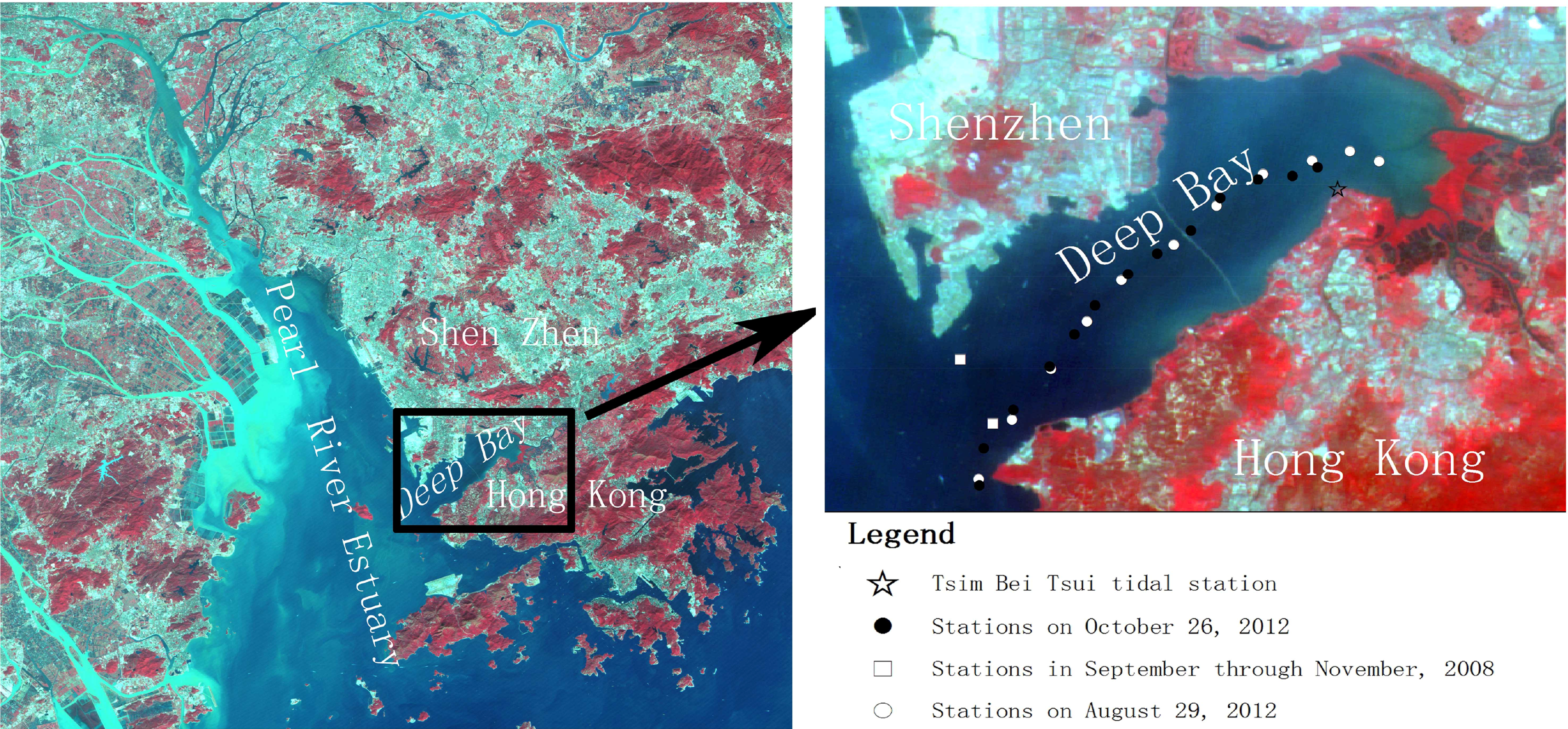
Deep Bay (22°24′18″N–22°32′12″N, 113°53′06″E–114°02′30″E) is a shallow, semi-enclosed bay situated on the east shore of the Pearl River Estuary, between Shenzhen to the north, which is a special economic zone of China, and the New Territories of Hong Kong to the south (Figure 1). The bay is 4–7.6 km wide and 13.9 km long, with a total sea surface area of approximately 80 km2. The dry season in this area is from October to March, whereas the wet season is from April to August. Deep Bay has a relatively flat sea bed, with a depth at the mouth of approximately 5 m [30]. Deep Bay has suffered from extensive anthropogenic pollutants emitted by villages and livestock farms [31]. A recent evaluation indicated that the water quality of Deep Bay was the worst among all the waters of Hong Kong [32], posing threats to the sensitive associated ecosystems (wetland reserves) and oyster culturing in the bay [33,34]. As the area around Deep Bay shows high potential for further development, it is essential to understand the sediment conditions of the bay.
Deep Bay is influenced by the subtropical oceanic monsoon climate and therefore receives abundant rainfall and is often affected by typhoons and storms. Thus, although the satellite images used for ocean color and water quality mapping must be atmospherically clear, such clear images are seldom available. Furthermore, the flood-ebb tidal cycle re-suspends bottom sediments and plays an important role in the variation of TSS conditions. Thus, it is challenging to dynamically monitor TSS activity in Deep Bay.
2.2. Data Sources
2.2.1. In-Situ Data
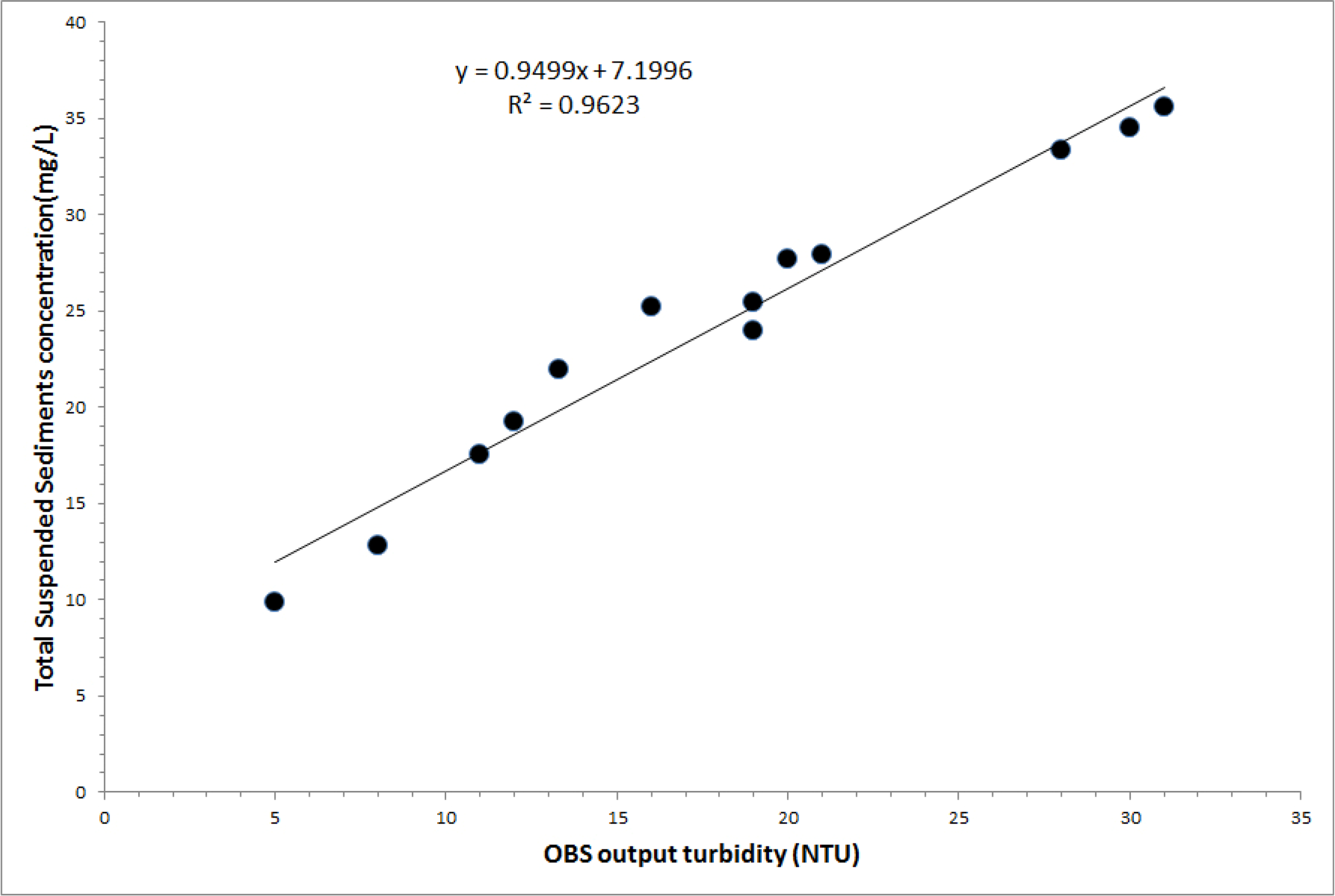
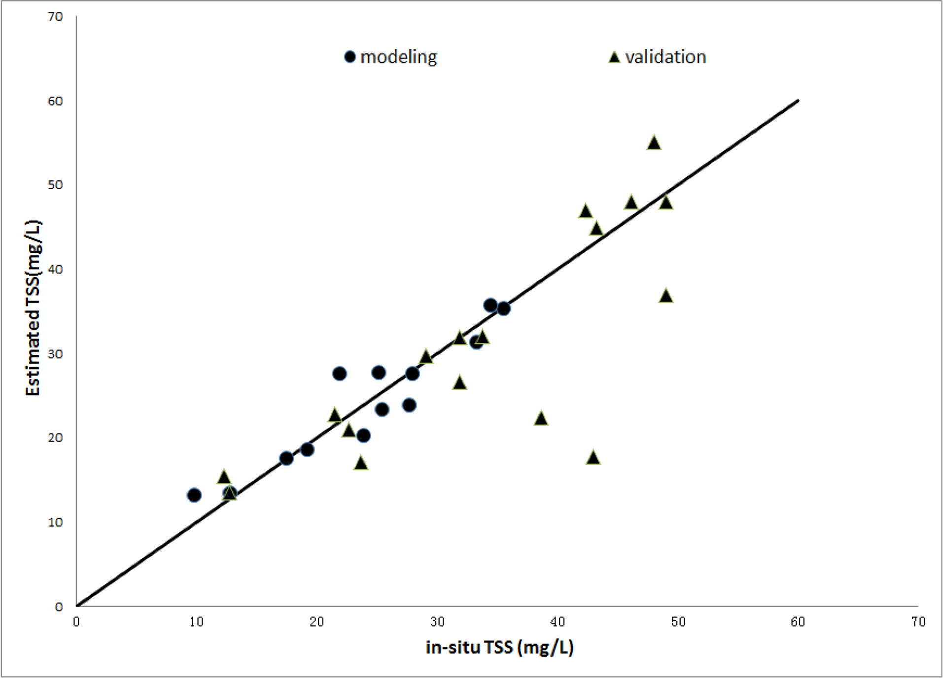
Two field surveys were conducted in Deep Bay. In Figure 1, the white circles represent the sampling stations visited on 29 August 2012, during the wet season, and the black circles represent the sampling stations visited on 26 October 2012, during the dry season. All field measurements were conducted between 10 A.M. and 1 P.M. local time to ensure that the in-situ data were comparable with the HJ-1A/1B satellite CCD measurements (Satellite Descending node: 10:30 A.M.). During these observations, an optical backscatter (OBS) sensor, which is an optical sensor for measuring turbidity and suspended sediment concentrations by detecting infrared light scattered from suspended matter, produced by the D & A Instrument Company [35], was operated nearly continuously (approximately 26 measurements in total), and 18 water samples for TSS analyses were simultaneously collected in 1 L plastic jugs for inter-comparison with the OBS sensor data to ensure that all of the TSS measurements are credible. Water samples were transported to the laboratory and filtered through 47 mm glass fiber filters to obtain the TSS concentration using a weighting method (Whatman GF/F with a 0.7 μm effective pore size). The regression results for the TSS concentrations obtained from water samples and OBS measurements are shown in Figure 2. The coefficient of determination, R2, for the relationship was 0.96, and the MRE was 6.45%. Long-term series-calibrated OBS measurements carried out at two stationary stations (see starred locations in Figure 1) from September through November 2008 were treated as the “ground truth” to test the stability of the algorithms and to assess the influence of meteorological-hydrological data. The northern stationary station was designated as K1, and the southern station was designated as A1.
The in-situ spectrum was also measured correctly in the wavelength range 200–1120 nm using a 0.065 nm full-width half-maximum (FWHM) Ocean Optics HR2000 fiber-optic spectrometer (Ocean Optics, Dunedin, FL, USA) [36], with the viewing direction of 40° from the nadir and 135° from the sun to minimize the effects of sun glint and non-uniform sky radiance while also avoiding instrument shading problems, following the NASA-recommended protocols for optical measurements [37,38]. The related dimensionless air-water reflectance was determined from previous work [37–40]. The measured remote sensing reflectance (Rrs, Sr−1) is calculated from the following equation:
2.2.2. Satellite Data
The simultaneous HJ-1A/1B CCD images obtained on both 29 August and 26 October 2012, were heavily contaminated with clouds. Hence, the cloud-free HJ-1A/1B CCD images generated on 28 August and 24 October 2012 were selected to retrieve TSS. In addition, the six cloud-free images collected on 10 October, 26 October, 7 December, 14 November, 15 December and 19 December 2008 were processed to show different TSS patterns under particular tide and wind conditions.
2.2.3. Meteorological and Hydrologic Data
The wind vectors measured at the Lau Fau Shan station (located on the southern shore of Deep Bay) in 2008 from the Hong Kong Observatory [41] were used for the analysis of meteorological factors’ effect on the TSS distribution. The hourly recorded wind data, including wind speeds and directions, were used to analyze the prevailing wind directions and average wind speed within the satellite’s imaging time. The corresponding half-hourly tidal height measured at the Tsim Bei Tsui tidal station (Figure 1), located at the Inner Deep Bay wetlands and the indented western coast of Hong Kong [42] was selected to characterize the tide of the Deep Bay and its relationship with the distribution of the TSS concentration.
3. Methodology
3.1. Atmospheric Correction
The COST method is very simple and popular among researchers, especially when there is no auxiliary information to support other physically based methods. Several studies have shown that the COST model can be used to remove atmospheric effects for water environment remote sensing applications [14,28,43]. However, the image-based method depends on the information provided by the selected image scene, and it can introduce uncertainties, altering the detection of satellite images on different dates, especially in dynamic atmospheric conditions. Furthermore, the images used in this study were collected by four different CCD sensors onboard the HJ-1A/1B satellites. Thus, radiation normalization based on pseudo-invariant features (PIF) is recommended before the retrieval model established for a specific day is extended in temporal space.
3.1.1 The COST (Cosine of the Sun Zenith Angle (cos(TZ))) Model
COST is an image-based absolute atmospheric correction method proposed for Landsat TM data [27]. This method uses only the cosine of the sun zenith angle (cos(TZ)) as an acceptable parameter for approximating the effects of atmospheric gas absorption and Rayleigh scattering, hence the name COST [44]. Similar to Landsat TM sensors, the COST method is effective for HJ-1A/1B satellite CCD images. The procedures are as follows:
- (1)
Conversion of digital numbers (DN) to the radiance at satellite (Lsat) using the gain and offset parameters from the image adjective XML file [45].
- (2)
Determination of the minimum DN for each reflective band. This value may be either the histogram minimum or a slightly higher value depending on image properties. Then, each minimum DN value is converted to an at-satellite minimum spectral radiance value:
where QCAL is the minimum DN, QCALMAX = 255 (8 bits) and the constants Lminλ and Lmaxλ are determined according to the method proposed by Markham and Moran [46].- (3)
Computation of the radiance of a dark object (assumed to have a reflectance of 1%) for each band [27]:
where ESUNλ = mean solar exo-atmospheric spectral irradiance, θ = solar zenith angle and d = earth-sun distance.- (4)
Application of haze correction:
- (5)
Reflectance at the sea surface is obtained after atmospheric correction:
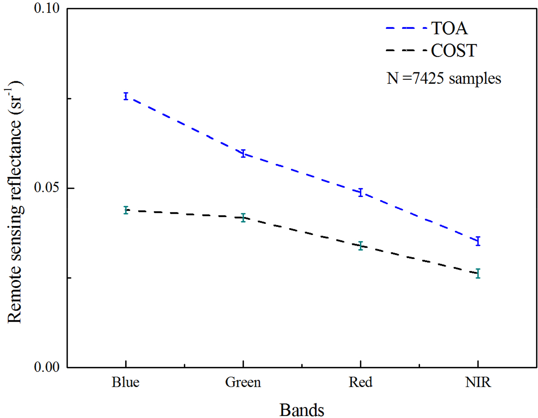
The Rrs(Sr−1) before and after atmospheric correction were compared in Figure 3, where the mean spectra were calculated using 7425 randomly selected pixels on HJ-1B satellite CCD2 imagery of 28 August 2012. As shown in Figure 3, the atmospherically corrected blue band (e.g., band 1) may not be satisfactory, which is similar to MODIS or other instruments. However, the performance of the green and red bands should be acceptable. The results are similar with the previous atmospheric correction evaluation work of HJ-1A/1B CCD images in Poyang Lake [47].
3.1.2. The Pseudo-Invariant Features Method
In 1988, Schott et al. [48] developed a relative radiometric normalization method using spectrally pseudo-invariant features (PIF), such as impervious roads, roof tops and parking lots, to allow for inter-comparisons between a target image and a base image by calculating an image-based linear regression. The PIF method has been tested at several study sites [49–53], especially in water areas with haze contamination [45]. In the present study, the relatively haze-free HJ-1A satellite CCD2 image obtained on 28 August 2012, was used as a reference, and certain pixels were singled out as the pseudo-invariant feature set via the temporally invariant cluster (TIC) method [54]. The relationship built on the target image and base image obtained on 28 August 2012, was used to perform radiation standardization of the cloud-free HJ-1A/1B satellite CCD measurements from 24 October 2012, and for the six images from September to November 2008.
3.2. Total Suspended Sediment Retrieval Model
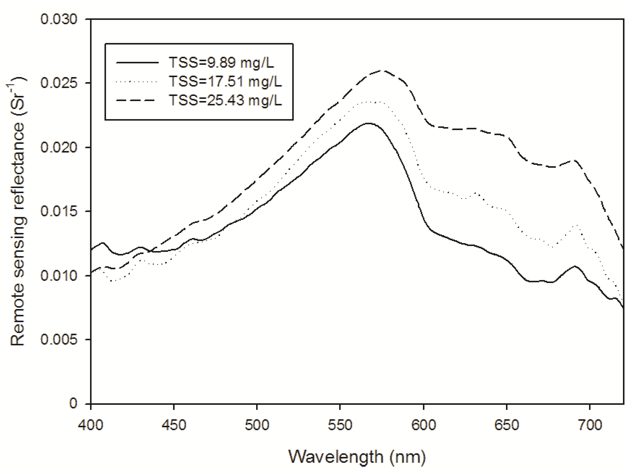
Several examples of Rrs and their corresponding TSS values are presented in Figure 4. Note that the reflectance peak near 550 nm and the reflectance platform between 600 nm and 650 nm significantly increased with the increase of the TSS concentration.
Regressions between in-situ TSS and remote sensing reflectance data (or the reflectance ratio) were derived to develop appropriate TSS algorithms. Figure 5 shows the regression relationships between in-situ TSS and Rrs2, Rrs3 and Rrs3/Rrs2. Among these regressions, the band-ratio exponent algorithm showed better performance than the single-band algorithm based on measures with a higher coefficient of determination (R2) and lower MRE because the influence of sediment grain size and refractive index variations on the reflectance in satellite bands is reduced when considering reflectance ratios [55].
According to the spectral characteristics of turbid waters, bands from 500 to 700 nm are effective for the retrieval of TSS concentrations from Landsat, SPOT and HJ-1A/1B satellite CCD sensors [7,10,16,27]. Considering previous work conducted in the Pearl River Estuary [56–58], the water area adjacent to Deep Bay, band 2 and band 3 are appropriate for TSS retrieval in this area. On the basis of the reasonable results regarding the in-situ-measured Rrs and TSS concentrations on 29 August 2012, the empirical algorithm with the highest coefficient of determination obtained through regression analysis among different band combination forms for TSS retrieval was established as follows (see Figure 5):
4. Results and Discussion
4.1. TSS Concentrations in Deep Bay
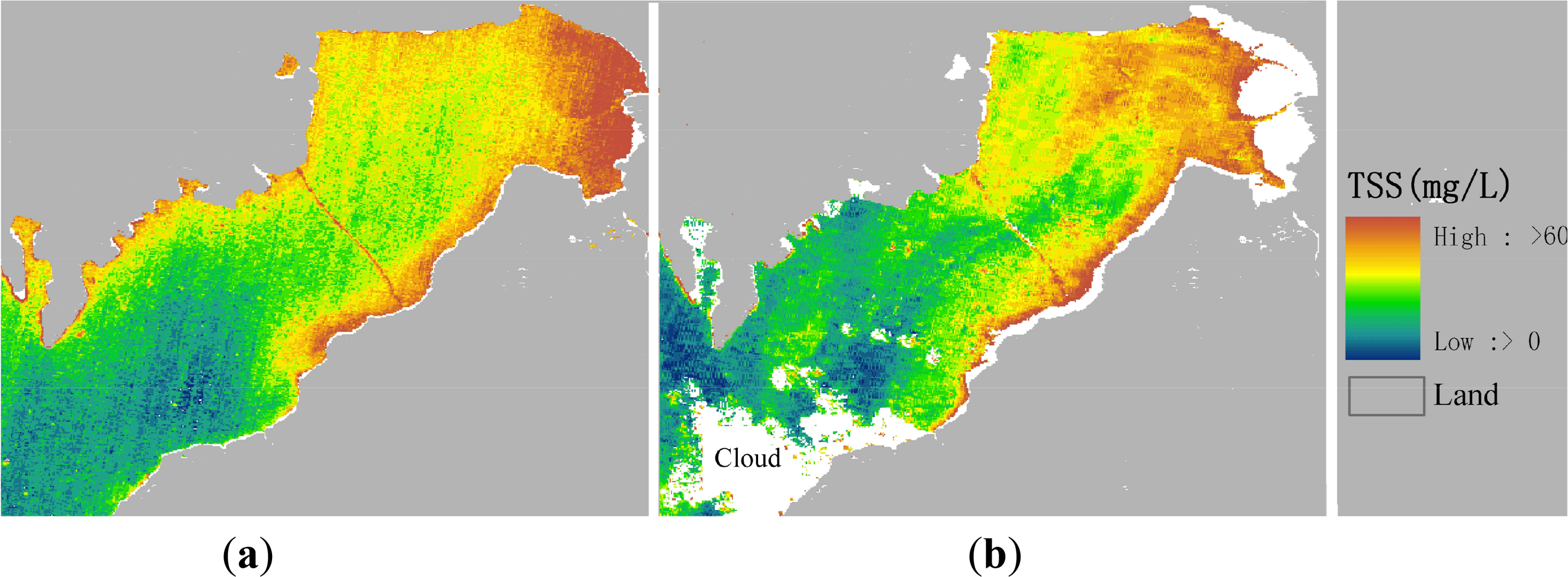
Prior to TSS retrieval, the very common normalized difference vegetation index (NDVI), defined as (RNIR–RRED)/(RNIR+RRED), which is typically lower for water than for land, was employed for water/land delineation [59]. Using the atmospheric correction results and the retrieval algorithm, the TSS distributions were derived from the HJ-1A/1B CCD images acquired on 28 August and 24 October 2012 (Figure 6). The retrieved results closely matched the in-situ data at each station (Figure 7). The modeling and validation match-ups could be found in Figure 7. The MRE between the calibrated OBS data and satellite TSS results was 15.0851%. The field measurements and HJ-1A/1B satellite CCD data were approximately 1–2 days apart; therefore, some disagreement is expected due to the temporal and spatial variability associated with the tide plume and the river discharge. The retrieved TSS patterns showed a similar distribution, with TSS decreasing spatially along the transect from the inner to the outer bay, and little disagreement can be observed in Figure 6. There is a turbid plume in the inner Deep Bay near the Shenzhen and Dasha Rivers. In this area, the TSS concentrations were greater than 20 mg/L, which is much higher than the threshold value of 10 mg/L above which primary production begins to become light limited [60,61]. The high turbidity may be partly caused by the discharge of these two rivers and, more importantly, the influence of the tide. The mouth of Deep Bay is relatively clearer than the other regions. The water with a low TSS concentration may be mixed with the adjacent ocean water because of the flood and ebb tides. Further investigation is needed to obtain a more detailed explanation.
4.2. Forces Driving the TSS Distribution in Deep Bay
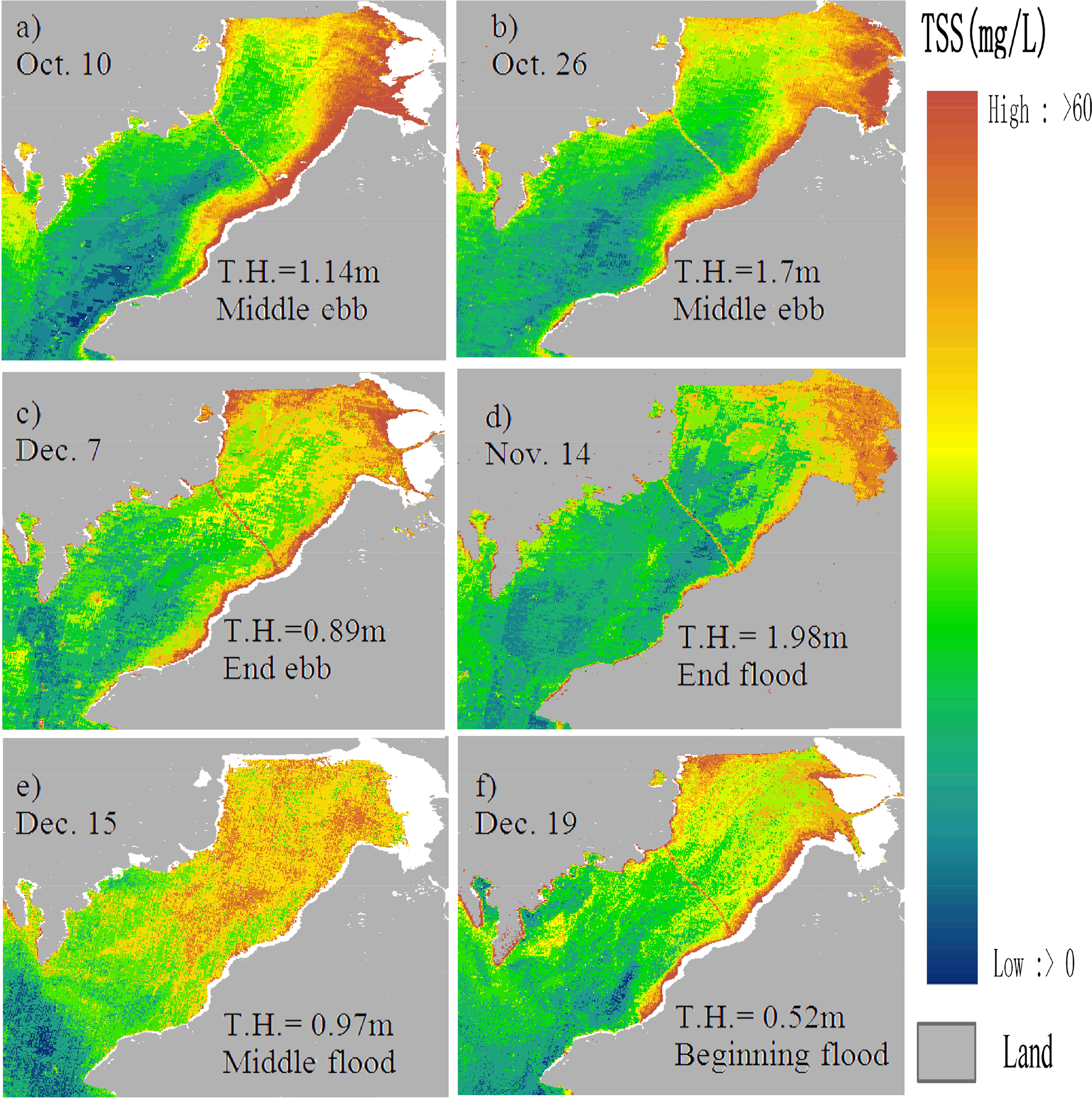
Six cloud-free HJ-1A/1B satellite CCD images obtained from September through November of 2008 were also processed to investigate the dynamics of the water environment in Deep Bay (Figure 8). The satellite retrieved TSS concentrations were validated with the 12 simultaneous in-situ OBS measurements in the stationary K1 and A1, and the relative error is about 27.8%. Large changes in the water area can be observed in Table 1 and Figure 8. As shown in Figure 8, a large range of tides occurred on 10 October, 26 October, 7 December, 14 November, 15 December and 19 December 2008. The mean tidal height on these six days in Deep Bay was approximately 1.25 m above Chart Datum at the Tsim Bei Tsui station and varied between 0.52 m and 1.98 m during flood-ebb tides. When the measured height of the tide was approximately 1.98 m on 14 November 2008 (Figure 8d), the water area was approximately 80.0775 km2, which was the largest area among these six observation days, nearly equal to the official total water surface area recorded. In contrast, the measured height of the tide was approximately 0.52 m on 19 November 2008, which was the lowest among these six images, and the water area was only approximately 69.0435 km2 (Figure 8f). The exposed tidal zone was approximately 11.034 km2 (blank area in Figure 8f), constituting 13.78% of the water area extracted from the satellite image collected on 14 November 2008.
The water area varied greatly, as did the TSS concentrations. As shown in Figure 8, the highest TSS concentration was always found in the east and southeast regions of Deep Bay near the coastline in these six images, but the TSS pattern in the central water area varied greatly. The spatial distribution of TSS presented in Figure 8 retrieved from the images collected on 10 October (Figure 8a), 26 October (Figure 8b) and 8 December (Figure 8c), 2008 reveals the pattern of the ebb tide and shows that the height of the tide above Chart Datum at Tsim Bei Tsui station was 1.14 m, 1.7 m and 0.89 m on these dates, respectively. The results obtained for the three dates displayed similar characteristics in that the TSS concentration was lower at the mouth and higher in the inner Deep Bay in most cases. However, the detailed spatial TSS distributions on these dates varied widely. The TSS distributions shown in Figure 8a and Figure 8b are from the middle progress of the ebb tide, whereas the TSS distribution shown in Figure 8c is from the end of the ebb tide, near low tide. The water depth near the coastline in the inner bay is lower than in other water bodies, and high turbidity can therefore be found in this area due to re-suspension caused by the greatest velocity in the process of ebb tide. In the central deeper water area near the mouth of Deep Bay, the suspended sediments are therefore higher because of the lower water depth near the coastline [62]; further investigation would be needed to discuss the cause of this formation in the future. We observed a non-turbid water plume at the central mouth of the bay. When the low tide arrived, the velocity became slower throughout the water area and the turbid water was able to disperse. Thus, the water body in the middle of the bay mouth would be more turbid (see Figure 8c). The TSS distributions recorded during flood tide are presented in Figure 8d,e,f. At the beginning of the flood tide, the spatial pattern (Figure 8f) obtained on 19 December 2008 was similar to that of the low tide (Figure 8c) observed on 7 December 2008. In contrast, in the middle of flood tide (Figure 8e), clear water from the outer sea entered the bay, the turbid water could not disperse to the ocean and the water became mixed in the bay (Figure 8e). A relatively clear water plume in the Pearl River Estuary can be observed in Figure 8e. However, the TSS concentration (Figure 8e) on 15 December 2008 was obviously much higher than on the other five dates. This difference may have been caused by the greater height of the tide cycle, varying from 0.06–2.96 m (see Figure 9c). The shallower the water is, the greater the amount of re-suspended sediments will be due to tidal hydraulic elements when other conditions have not changed. With the progress of the flood tide, the turbid water in the central bay would be mixed with clear ocean water near high tide. The turbid water would appear in the inner bay near the coastal water (see Figure 8d). After the high tide, a similar spatial distribution would reappear during ebb tide, as shown in Figure 8a and Figure 8b. The results derived from the HJ-1A/1B satellite CCD sensors may represent the TSS temporal and spatial variation during an uncommon tidal cycle.
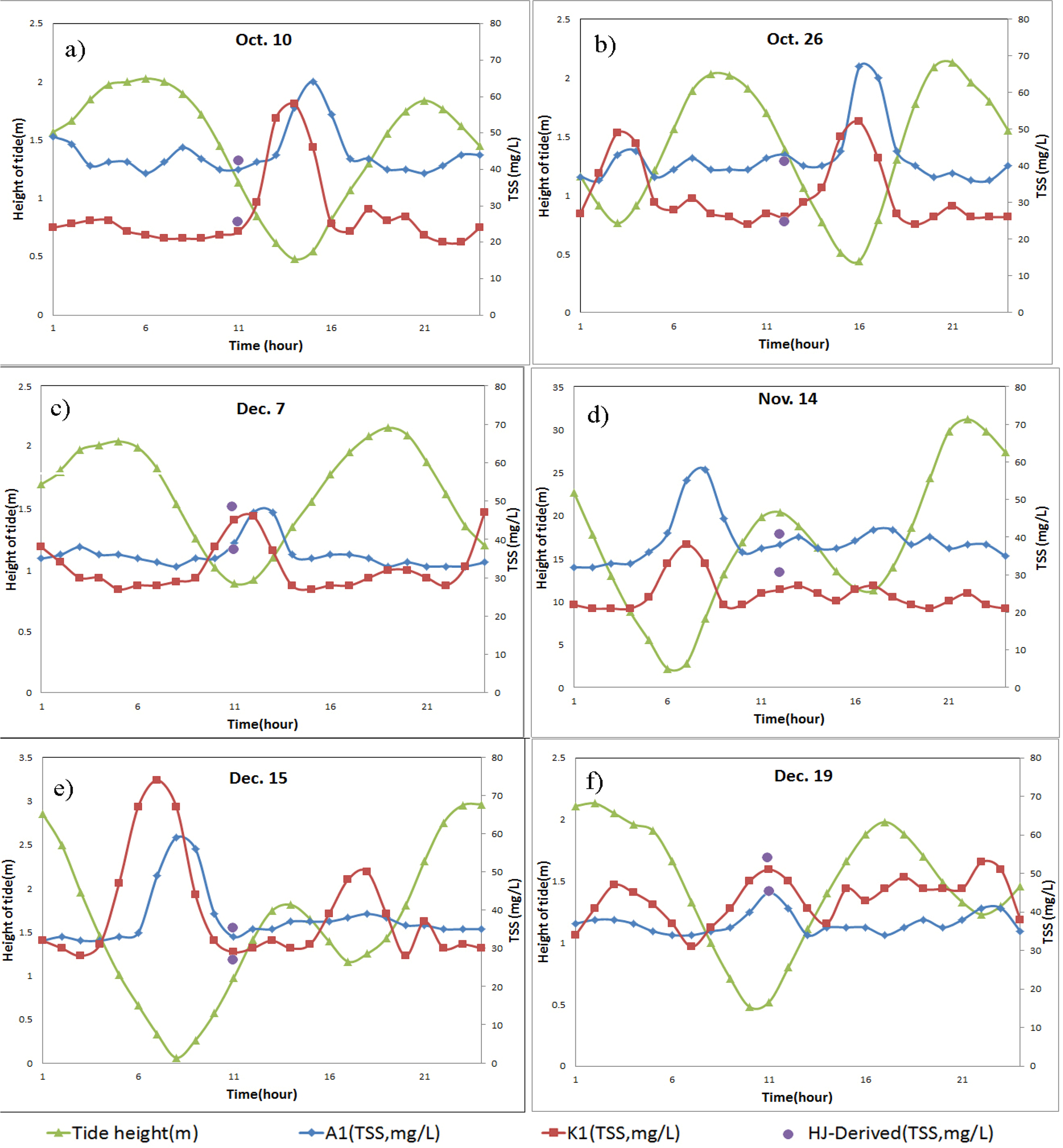
To support the above analysis, the measured height of the tide above Chart Datum at Tsim Bei Tsui station and the OBS measurements obtained at the A1 and K1 stations on 10 October, 26 October, 7 December, 14 November, 19 December and 15 December 2008 are also displayed here. A good correlation between the TSS concentrations and the height of the tide can be observed in Figure 9. The phenomenon observed using HJ-1A/1B satellite data is very similar to the OBS observations made at stations A1 and K1 in 2008. From Figure 9, we can see that the highest TSS concentration always appears near low tide, whereas the lowest turbidity always occurs near high tide. In addition, the OBS measurements recorded near low tide on 15 December 2008 are higher than those on the other five dates. The simultaneous range of the spring tide can also be found in Figure 9e (0.06–2.96 m).
However, disagreements among measurements still exist, which may be partly caused by other factors, including the wind speed, wind direction, water depth, ships and other factors such as floating rafts for the artificial propagation of oysters. The meteorological data recorded hourly at Lau Fau Shan station were used to analyze the relationship between the wind and the distribution of TSS. For each single image, the wind speed and direction within the imaging time during the week were selected. There were two main wind directions on these days: southward and westward. On 10 October, 26 October and 7 December, the prevailing wind direction was southward and the maximum wind speed was approximately 5–6 m/s. The southward wind might strengthen sediment transport from the north shore to the south and cause re-suspension in the shallow waters off the south shore. Therefore, a higher TSS concentration was observed along the south shore. While the prevailing wind direction was westward (14 November and 15 December), sediment could be more easily transported from the east shore to the inner Deep Bay, decreasing the variation in TSS concentrations between the east shore and the inner Deep Bay. It is difficult to interpret the complicated causes of the TSS distribution variation just using one or two observed factors. Additional hydrological information and models are needed to verify the reason for the observed variation in TSS in detail.
5. Conclusions
In this study, a good linear relationship with a coefficient of determination, R2, of 0.9623 was found between the OBS field measurements and the laboratory-analyzed TSS concentrations in Deep Bay obtained during the two surveys conducted on 28 August and 26 October 2012. The proposed method of combining the COST method with PIF atmospheric correction was proved to be effective in processing long-time-series HJ-1A/1B satellite CCD images, even without aerosol and spectrum information support. A retrieval model was established using the corrected band reflectance ratio (Rrs3/Rrs2) and calibrated OBS TSS concentration data to reduce the cumulative effect of the atmospheric correction error. We focused on the influence of meteorological-hydrological data to explain the variation of the TSS distribution. The six results retrieved from HJ-1A/1B satellite CCD images from September through November of 2008 showed that the flood-ebb tidal cycle is one of the major factors inducing the temporal and spatial variation of TSS and that wind direction, wind speed and floating objects in the water may also influence the TSS distribution; however, further investigations should be conducted. Although there are still many problems to be investigated, we believe that the results of the present study will be helpful for dynamically and quantitatively monitoring turbid waters via remote sensing. Our findings will also be useful for performing numerical simulations and further ecological environmental studies.
In future work, more effective atmospheric correction and remote sensing retrieval models based on physical theory will be used to process images from different satellite sensors to monitor the water environment with a higher spatial and temporal resolution. In addition, the coupling of remote sensing and numerical simulations to study suspended sediment concentrations under comprehensive conditions will be undertaken.
Acknowledgments
This work was supported by the Open Research Fund of Key Laboratory of Digital Earth Science, Institute of Remote Sensing and Digital Earth, Chinese Academy of Sciences (No. 2013LDE004); the National Basic Research Program (973 Program) (No. 2011CB707106); the Program for Changjiang Scholars and Innovative Research Team in University (IRT1278); the National 863 Key Project (2012AA12A304); the Hong Kong Research Grants Council (RGC) General Research Fund (Grant No. B-Q23G); the National Natural Science Foundation of China (Nos. 41331174, 41071261, 40906092, 40971193, 41101415, 41401388 and 41406205) the Major Science and Technology Program for Water Pollution Control and Treatment (2013ZX07105-005); LIESMARS Special Research Funding; the ‘985 Project’ of Wuhan University; and special funds from the State Key Laboratory for equipment. A special thanks is to Chuqun Chen and Shiling Tang (South China Sea Institute of Oceanology, Chinese Academy of Sciences), for their support in the field investigation. The authors are grateful to the participants in the field investigation for data collection, especially those who carried out stationary station data collection. The authors would like to express their thanks to the China Centre for Satellite Data Resources and Application and Hong Kong Observation for the satellite and meteorological data.
Authors Contributions
Liqiao Tian conceived the study, Onyx W. H. Wai and Xiaoling Chen supported the study and the field investigation, Yaohui Liu helped to prepare the field data, Jiang Li and Jue huang analyzed the data, Liqiao Tian and Lian Feng prepared and revised the manuscript, and all authors discussed the results and commented on the manuscript.
Conflicts of Interest
The authors declare no conflict of interest.
References
- Zhou, M.-J.; Zhu, M.-Y. “Progress of the project” ecology and oceanography of harmful algal blooms in China. Adv. Earth Sci 2006, 21, 673–679. (In Chinese). [Google Scholar]
- Hu, C.-M.; Lee, Z.-P.; Ma, R.-H.; Yu, K.; Li, D.-Q.; Shang, S.-L. Moderate resolution imaging spectroradiometer (MODIS) observations of cyanobacteria blooms in Taihu Lake, China. J. Geophys. Res.: Oceans 1978–2012 2010, 115. [Google Scholar] [CrossRef]
- Duan, H.-T.; Zhang, S.-X.; Zhang, Y.-Z. Cyanobacteria bloom monitoring with remote sensing in Lake Taihu. J. Lake Sci 2008, 20, 145–152. [Google Scholar]
- Tan, Y.-H.; Huang, L.-M.; Chen, Q.-C.; Huang, X.-P. Seasonal variation in zooplankton composition and grazing impact on phytoplankton standing stock in the Pearl River Estuary, China. Cont. Shelf Res 2004, 24, 1949–1968. [Google Scholar]
- Cloern, J.E.; Jassby, A.D. Patterns and scales of phytoplankton variability in estuarine—Coastal ecosystems. Estuaries and Coasts 2010, 33, 230–241. [Google Scholar]
- Hu, C.-M.; Chen, Z.-Q.; Clayton, T.D.; Swarzenski, P.; Brock, J.C.; Muller-Karger, F.E. Assessment of estuarine water-quality indicators using MODIS medium-resolution bands: Initial results from Tampa Bay, FL. Remote Sens. Environ 2004, 93, 423–441. [Google Scholar]
- Yu, Z.-F.; Chen, X.-L.; Zhou, B.; Tian, L.-Q.; Yuan, X.-H.; Feng, D. Assessment of total suspended sediment concentrations in Poyang Lake using HJ-1A/1B CCD imagery. Chin. J. Oceanol. Limnol 2012, 30, 295–304. [Google Scholar]
- Feng, L.; Hu, C.-M.; Chen, X.-L.; Tian, L.-Q.; Chen, L.-Q. Human induced turbidity changes in Poyang Lake between 2000 and 2010: Observations from MODIS. J. Geophys. Res.: Oceans 2012, 117, 1978–2012. [Google Scholar] [CrossRef]
- Dekker, A.G.; Vos, R.J.; Peters, S.W.M. Comparison of remote sensing data, model results and in situ data for total suspended matter (TSM) in the southern Frisian lakes. Sci. Total Environ 2001, 268, 197–214. [Google Scholar]
- Dekker, A.G.; Vos, R.J.; Peters, S.W.M. Analytical algorithms for lake water TSM estimation for retrospective analyses of TM and SPOT sensor data. Int. J. Remote Sens 2002, 23, 15–35. [Google Scholar]
- Doxaran, D.; Froidefond, J.-M.; Lavender, S.; Castaing, P. Spectral signature of highly turbid waters: Application with SPOT data to quantify suspended particulate matter concentrations. Remote Sens. Environ 2002, 81, 149–161. [Google Scholar]
- Doxaran, D.; Froidefond, J.-M.; Castaing, P. A reflectance band ratio used to estimate suspended matter concentrations in sediment-dominated coastal waters. Int. J. Remote Sens 2002, 23, 5079–5085. [Google Scholar]
- Klemas, V.; Bartlett, D.; Philpot, W. Coastal and estuarine studies with ERTS-1 and Skylab. Remote Sens. Environ 1974, 3, 153–174. [Google Scholar]
- Min, J.-E.; Ryu, J.-H.; Lee, S.; Son, S. Monitoring of suspended sediment variation using Landsat and MODIS in the Saemangeum coastal area of Korea. Mar. Pollut. Bull 2012, 64, 382–390. [Google Scholar]
- Moore, G.F.; Aiken, J.; Lavender, S.J. The atmospheric correction of watercolour and the quantitative retrieval of suspended particulate matter in Case II waters: Application to MERIS. Int. J. Remote Sens. 1999, 20, 1713–1733. [Google Scholar]
- Ritchie, J.C.; Cooper, C.M.; Schiebe, F.R. The relationship of MSS and TM digital data with suspended sediments, chlorophyll, and temperature in Moon Lake, Mississippi. Remote Sens. Environ. 1990, 33, 137–148. [Google Scholar]
- Song, K.-S.; Li, L.; Wang, Z.-M.; Liu, D.-W.; Zhang, B.; Xu, J.-P.; Du, J.; Li, L.-H.; Li, S.; Wang, Y.-D. Retrieval of total suspended matter (TSM) and chlorophyll-a (Chl-a) concentration from remote-sensing data for drinking water resources. Environ. Monit. Assess 2012, 184, 1449–1470. [Google Scholar]
- Tassan, S. An improved in-water algorithm for the determination of chlorophyll and suspended sediment concentration from Thematic Mapper data in coastal waters. Int. J. Remote Sens 1993, 14, 1221–1229. [Google Scholar]
- Tassan, S. Local algorithms using SeaWiFS data for the retrieval of phytoplankton, pigments, suspended sediment, and yellow substance in coastal waters. Appl. Opt 1994, 33, 2369–2378. [Google Scholar]
- Salama, M.S.; Shenm, F. Simultaneous atmospheric correction and quantification of suspended particulate matters from orbital and geostationary earth observation sensors. Estuar. Coast. Shelf Sci 2010, 86, 499–511. [Google Scholar]
- Shen, F.; Verhoef, W.; Zhou, Y.-X.; Salama, M.S.; Liu, X.-L. Satellite estimates of wide-range suspended sediment concentrations in Changjiang (Yangtze) estuary using MERIS data. Estuaries and Coasts 2010, 33, 1420–1429. [Google Scholar]
- China Centre for Resources Satellite Data and Application (CRESDA). The Introduce for HJ-1-A, B Satellite. Available online: http://www.cresda.com/n16/n1130/n1582/8384.html (accessed on 8 May 2009).
- Xu, W.; Gong, J.-Y.; Wang, M. Development, application, and prospects for Chinese land observation satellites. Geo-spat. Inf. Sci 2014, 17, 102–109. [Google Scholar]
- Wang, M.H.; Shi, W. The NIR-SWIR combined atmospheric correction approach for MODIS ocean color data processing. Opt. Express 2007, 15, 15722–15733. [Google Scholar]
- Tian, L.-Q.; Lu, J.-Z.; Chen, X.-L.; Yu, Z.-F.; Xiao, J.-J.; Qiu, F.; Zhao, X. Atmospheric correction of HJ-1A/B CCD images over Chinese coastal waters using MODIS-Terra aerosol data. Sci. China Technol. Sci 2010, 53, 191–195. [Google Scholar]
- Lu, D.; Mausel, P.; Brondizio, E.; Moran, E. Assessment of atmospheric correction methods for Landsat TM data applicable to Amazon basin LBA research. Int. J. Remote Sens 2002, 23, 2651–2671. [Google Scholar]
- Chavez, P.S. Image-based atmospheric corrections-revisited and improved. Photogramm. Eng. Remote Sens 1996, 62, 1025–1035. [Google Scholar]
- Han, L.-H.; Jordan, K.J. Estimating and mapping chlorophyll—A concentration in Pensacola Bay, Florida using Landsat ETM+ data. Int. J. Remote Sens 2005, 26, 5245–5254. [Google Scholar]
- Miller, R.L.; McKee, B.A. Using MODIS Terra 250 m imagery to map concentrations of total suspended matter in coastal waters. Remote Sens. Environ 2004, 93, 259–266. [Google Scholar]
- Wong, S.H.; Li, Y.S. Hydrographic surveys and sedimentation in Deep Bay, Hong Kong. Environ. Geol 1990, 15, 111–118. [Google Scholar]
- EPD. Marine Water Quality in Hong Kong in 2004. Available online: http://www.epd.gov.hk/epd/english/environmentinhk/water/river_quality/rwq_report.html (accessed on 30 May 2014).
- EPD. Marine Water Quality in Hong Kong in 2006. Available online: http://www.epd.gov.hk/epd/english/environmentinhk/water/river_quality/rwq_report.html (accessed on 30 May 2014).
- Lee, J.H.; Qian, A.G. Three-dimensional modeling of hydrodynamic and flushing in deep bay. In Proceeding of International Conference on Estuaries and Coasts, Hangzhou, China, 9–11 November 2003.
- Xu, J.; Yin, K.-D.; Lee, J.H.W.; Liu, H.-B.; Ho, A.Y.T.; Yuan, X.-C.; Harrison, P.J. Long-term and seasonal changes in nutrients, phytoplankton biomass, and dissolved oxygen in Deep Bay, Hong Kong. Estuaries and Coasts 2010, 33, 399–416. [Google Scholar]
- Campbell Scientific, Inc. The Introduce for OBS Sensor. Available online: http://www.d-a-instruments.com/obs3a.html (accessed on 17 June 2014).
- Ocean Optics. HR Series. Available online: http://oceanoptics.com/product-category/hr-series/ (accessed on 17 June 2014).
- Lee, Z.; Carder, K.L.; Steward, R.G. Protocols for Measurement of Remote-Sensing Reflectance from Clear to Turbid Waters; SeaWiFS Workshop: Halifax, Nova Scotia, Canada, 1996. [Google Scholar]
- Mobley, C.D. Estimation of the remote-sensing reflectance from above-surface measurements. Appl. Opt 1999, 38, 7442–7455. [Google Scholar]
- Hale, G.M.; Querry, M.R. Optical constants of water in the 200-nm to 200-µm wavelength region. Appl. Opt 1973, 12, 555–563. [Google Scholar]
- Tang, J.-W.; Tian, G.L.; Wang, X.Y.; Wang, X.M.; Song, Q.J. The methods of water spectra measurement and analysis I: Above-water method. J. Remote Sens.-Beijing- 2004, 48, 37–44. [Google Scholar]
- Hong Kong Observatory. Available online: http://www.hko.gov.hk/ (accessed on 17 June 2014).
- AEON JUSCO Education and Environment Fund. The Introduce for the Tsim Bei Tsuis station. Available online: http://www.aeonfund.org.hk/en/green_horizon/green_family_4.html (accessed on 15 October 2012).
- Islam, M.R.; Begum, S.F.; Yamaguchi, Y.; Ogawa, K. Distribution of suspended sediment in the coastal sea off the Ganges–Brahmaputra River mouth: Observation from TM data. J. Mar. Syst 2002, 32, 307–321. [Google Scholar]
- Mahiny, A.S.; Turner, B.J. A comparison of four commonatmospheric correction methods. Photogramm. Eng. Remote Sens 2007, 24. [Google Scholar] [CrossRef]
- Chavez, P.S., Jr. An improved dark-object subtraction technique for atmosphericscattering correction of multispectral data. Remote Sens. Environ 1988, 3, 459–479. [Google Scholar]
- Markham, B.L.; Barker, J.L. Landsat MSS and TM post-calibration dynamic ranges, exoatmosphericreflectances and at-satellite temperatures. EOSAT Landsat Tech. Notes 1986, 1, 3–8. [Google Scholar]
- Zeng, Q.; Zhao, Y.; Tian, L.Q.; Chen, X.L. Evaluation on the atmospheric correction methods for water color remote sensing by using HJ-1A/1B CCD image—Taking Poyang Lake in China as a Case. Spectrosc. Spectr. Anal 2013, 33, 1320–1326. (In Chinese). [Google Scholar]
- Schott, J.R.; Salvaggio, C.; Volchok, W.J. Radiometric scene normalization using pseunvariant features. Remote Sens. Environ 1988, 26, 1–16. [Google Scholar]
- Hadjimitsis, D.G.; Clayton, C.R.I.; Retalis, A. The use of selected pseudo-invariant targets for the application of atmospheric correction in multi-temporal studies using satellite remotely sensed imagery. Int. J. Appl. Earth Obs. Geoinf 2009, 11, 192–200. [Google Scholar]
- Ji, C.Y. Haze reduction from the visible bands of Landsat TM and ETM+ images over a shallow water reef environment. Remote Sens. Environ 2008, 112, 1773–1783. [Google Scholar]
- Pettit, N.E.; Jardine, T.D.; Hamilton, S.K.; Sinnamon, V.; Valdez, D.; Davies, P.M.; Douglas, M.M.; Bunn, S.E. Seasonal changes in water quality and macrophytes and the impact of cattle on tropical floodplain waterholes. Mar. Freshw. Res 2012, 63, 788–800. [Google Scholar]
- Sass, G.Z.; Creed, I.F.; Bayley, S.E.; Devito, K.J. Understanding variation in trophic status of lakes on the Boreal Plain: A 20 year retrospective using Landsat TM imagery. Remote Sens. Environ 2007, 109, 127–141. [Google Scholar]
- Ward, D.P.; Hamilton, S.K.; Jardine, T.D.; Pettit, N.E.; Tews, E.K.; Olley, J.M.; Bunn, S.E. Assessing the seasonal dynamics of inundation, turbidity, and aquatic vegetation in the Australian wet–dry tropics using optical remote sensing. Ecohydrology 2013, 6, 312–323. [Google Scholar]
- Chen, X.X.; Vierling, L.; Deering, D. A simple and effective radiometric correction method to improve landscape change detection across sensors and across time. Remote Sens. Environ 2005, 98, 63–79. [Google Scholar]
- Doxaran, D.; Froidefond, J.-M.; Castaing, P. Remote-sensing reflectance of turbid sediment-dominated waters. Reduction of sediment type variations and changing illumination conditions effects by use of reflectance ratios. Appl. Opt 2003, 42, 2623–2634. [Google Scholar]
- Liu, F.-F.; Chen, C.-Q.; Tang, S.-L. A piecewise algorithm for retrieval of suspended sediment concentration based on in situ spectral data by MERIS in Zhujiang River estuary. J. Trop. Oceanogr 2009, 28, 9–14. [Google Scholar]
- Tang, S.-L.; Qing, D.; Chen, C.-Q.; Liu, F.-F.; Jin, G.-Y. Retrieval of suspended sediment concentration in the Pearl River Estuary from MERIS using support vector machines. In Proceedings of 2009 IEEE International Geoscience and Remote Sensing Symposium, IGARSS 2009, Cape Town, South Africa, 12–17 July 2009; pp. III-239–III-242.
- Xi, H.-Y.; Zhang, Y.-Z. Total suspended matter observation in the Pearl River estuary from in situ and MERIS data. Environ. Monit. Assess 2011, 177, 563–574. [Google Scholar]
- Lunetta, R.S.; Knight, J.F.; Ediriwichrema, J.; Lyon, J.G.; Worthy, L.D. Land-cover change detection using multi-temporal MODIS NDVI data. Remote Sens. Environ 2006, 105, 142–154. [Google Scholar]
- Ragueneau, O.; Lancelot, C.; Egorov, V.; Vervlimmeren, J.; Cociasu, A.; Déliat, G.; Krastev, A.; Daoud, N.; Rousseau, V.; Popovitchev, V.; et al. Biogeochemical transformations of inorganic nutrients in the mixing zone between the Danube River and the north-western Black Sea. Estuar. Coast. Shelf Sci 2002, 54, 321–336. [Google Scholar]
- Soetaert, K.; Middelburg, J.J.; Heip, C.; Meire, P.; Damme, S.V.; Maris, T. Long-term change in dissolved inorganic nutrients in the heterotrophic Scheldt estuary (Belgium, The Netherlands). Limnol. Oceanogr 2006, 51, 409–423. [Google Scholar]
- Zhang, P.; Wai, O.W.; Chen, X.; Lu, J.; Tian, L. Improving sediment transport prediction by assimilating satellite images in a tidal bay model of Hong Kong. Water 2014, 6, 642–660. [Google Scholar]


| Date | Measured Height of the Tide (m) | Water Area (km2) | Exposed Tidal Zone (km2) | Percent of the Exposed Tidal Zone (%) |
|---|---|---|---|---|
| 10-Oct | 1.14 | 72.9783 | 7.0992 | 8.87 |
| 26-Oct | 1.7 | 78.9795 | 1.098 | 1.37 |
| 14-Nov | 1.98 | 80.0775 | 0 | 0 |
| 7-Dec | 0.89 | 71.1558 | 8.9217 | 11.14 |
| 15-Dec | 0.97 | 71.8524 | 8.2251 | 10.27 |
| 19-Dec | 0.52 | 69.0435 | 11.034 | 13.78 |
© 2014 by the authors; licensee MDPI, Basel, Switzerland This article is an open access article distributed under the terms and conditions of the Creative Commons Attribution license (http://creativecommons.org/licenses/by/4.0/).
Share and Cite
Tian, L.; Wai, O.W.H.; Chen, X.; Liu, Y.; Feng, L.; Li, J.; Huang, J. Assessment of Total Suspended Sediment Distribution under Varying Tidal Conditions in Deep Bay: Initial Results from HJ-1A/1B Satellite CCD Images. Remote Sens. 2014, 6, 9911-9929. https://0-doi-org.brum.beds.ac.uk/10.3390/rs6109911
Tian L, Wai OWH, Chen X, Liu Y, Feng L, Li J, Huang J. Assessment of Total Suspended Sediment Distribution under Varying Tidal Conditions in Deep Bay: Initial Results from HJ-1A/1B Satellite CCD Images. Remote Sensing. 2014; 6(10):9911-9929. https://0-doi-org.brum.beds.ac.uk/10.3390/rs6109911
Chicago/Turabian StyleTian, Liqiao, Onyx W. H. Wai, Xiaoling Chen, Yaohui Liu, Lian Feng, Jian Li, and Jue Huang. 2014. "Assessment of Total Suspended Sediment Distribution under Varying Tidal Conditions in Deep Bay: Initial Results from HJ-1A/1B Satellite CCD Images" Remote Sensing 6, no. 10: 9911-9929. https://0-doi-org.brum.beds.ac.uk/10.3390/rs6109911