Landsat 8 Thermal Infrared Sensor Geometric Characterization and Calibration

Abstract

The Landsat 8 spacecraft was launched on 11 February 2013 carrying two imaging payloads: the Operational Land Imager (OLI) and the Thermal Infrared Sensor (TIRS). The TIRS instrument employs a refractive telescope design that is opaque to visible wavelengths making prelaunch geometric characterization challenging. TIRS geometric calibration thus relied heavily on on-orbit measurements. Since the two Landsat 8 payloads are complementary and generate combined Level 1 data products, the TIRS geometric performance requirements emphasize the co-alignment of the OLI and TIRS instrument fields of view and the registration of the OLI reflective bands to the TIRS long-wave infrared emissive bands. The TIRS on-orbit calibration procedures include measuring the TIRS-to-OLI alignment, refining the alignment of the three TIRS sensor chips, and ensuring the alignment of the two TIRS spectral bands. The two key TIRS performance metrics are the OLI reflective to TIRS emissive band registration accuracy, and the registration accuracy between the TIRS thermal bands. The on-orbit calibration campaign conducted during the commissioning period provided an accurate TIRS geometric model that enabled TIRS Level 1 data to meet all geometric accuracy requirements. Seasonal variations in TIRS-to-OLI alignment have led to several small calibration parameter adjustments since commissioning.

1. Introduction

The Landsat 8 spacecraft, launched on 11 February 2013, continues the moderate resolution Earth imaging mission of the Landsat series that has been ongoing since the launch of Landsat 1 in 1972. Unlike the previous member of the Landsat family, Landsat 7, which collects multispectral image data in the visible and near infrared (VNIR), short-wave infrared (SWIR), and long-wave thermal infrared portions of the electromagnetic spectrum using a single cross-track scanning instrument—the Enhanced Thematic Mapper Plus (ETM+); Landsat 8 employs two separate imaging payloads. The Operational Land Imager (OLI) provides coverage of the VNIR and SWIR portions of the spectrum while the Thermal Infrared Sensor (TIRS) adds two long-wave thermal spectral channels [1], one centered at 10.9 micrometers (band 10) and a second centered at 12.0 micrometers (band 11). The data from both instruments are combined to create integrated Landsat 8 image data products. Ensuring the geometric registration of the OLI and the TIRS data is critical to Landsat 8 product quality.

The OLI and TIRS are both linear array push-broom instruments that continuously collect the full instrument cross-track field of view, accumulating a two-dimensional image as the spacecraft’s orbital motion carries it across the Earth’s surface. The OLI design, construction [2] and geometric calibration and performance [3] have been documented elsewhere. This paper describes the geometric modeling, calibration, and performance characterization activities that enable the geometric correction of TIRS data, and shows the on-orbit accuracy characterization results observed for the TIRS from launch through the first year of operation.

1.1. TIRS Overview

Details of the TIRS instrument design and construction have been provided separately [4] but there are several aspects of the TIRS design that are important to an understanding of the geometric models used in TIRS data processing and instrument geometric calibration. The TIRS employs three quantum well infrared photodiode (QWIP) detector arrays on a single cold (~40 Kelvin) focal plane to provide coverage of the full 185-kilometer cross-track instrument field of view at a nominal 100-meter ground sample distance. The detector arrays, spectral filters, and supporting electronics are packaged into three sensor chip assemblies (SCAs) that each cover approximately one-third of the field of view. The three SCAs are illuminated by a telescope subsystem that uses refractive optics to focus the incoming radiation on the focal plane. The use of refractive, rather than reflective, optics had important consequences for prelaunch characterization and calibration since it renders the TIRS telescope opaque to visible wavelengths of light. In order to support on-orbit radiometric calibration operations a flat mirror on a movable scene select mechanism (SSM) sits in front of the TIRS telescope. The SSM can be rotated to direct the telescope field of view toward the Earth, toward an on-board black body calibration source, or through a port on the cold side of the instrument that points to deep space. This movable mirror provides a potential source of short-term pointing variability and/or longer-term alignment instability. The key elements of the TIRS instrument design are shown in Figure 1.

Figure 1. Cutaway view of the Thermal Infrared Sensor (TIRS) instrument design showing major subsystems including: scene select mechanism; telescope and focal plane assembly (FPA); cryocooler.

Figure 1. Cutaway view of the Thermal Infrared Sensor (TIRS) instrument design showing major subsystems including: scene select mechanism; telescope and focal plane assembly (FPA); cryocooler.

1.2. Geometric Calibration Approach

The geometric algorithms and associated parameters required to perform accurate geometric correction and calibration for TIRS data are based upon an underlying sensor line-of-sight model that relates each TIRS imaging detector to a corresponding direction relative to the Landsat 8 spacecraft coordinate system. Constructing this line-of-sight model requires knowledge of the locations of each active detector on the TIRS focal plane, knowledge of the optical behavior of the TIRS telescope and scene select mechanism as they direct the lines-of-sight out the TIRS aperture, and knowledge of the alignment relationship between the TIRS instrument and the spacecraft attitude control system. An initial version of this line-of-sight model was constructed based upon TIRS design information prior to the beginning of instrument fabrication and assembly. This initial model was used to support algorithm development and initial data simulation exercises.

The initial design-based geometric model parameters were updated to reflect the as-built TIRS hardware using measurements taken during instrument-level thermal vacuum testing. This prelaunch characterization and analysis is described below in Section 2. The resulting prelaunch geometric line-of-sight model had relatively large uncertainties due to ongoing changes to the TIRS hardware configuration throughout the prelaunch testing process and also due to questions about the stability of the ground support equipment used to make the measurements. These questions arose because of the lack of repeatability that was observed across multiple test sequences.

Although a rigorous on-orbit geometric calibration campaign was always planned for the TIRS instrument, the uncertainties in the prelaunch calibration measurements heightened the importance of the on-orbit methods. Fortunately, having the geometrically stable OLI instrument acquiring data at the same time as the TIRS simplified the on-orbit calibration problem by providing an accurate reference for TIRS-to-OLI and TIRS internal alignment measurements. The TIRS on-orbit calibration program is described below in Section 3.

1.3. Geometric Performance Metrics

The ultimate objective of the TIRS geometric calibration process is to ensure that the TIRS data products meet their geometric accuracy requirements. These requirements are summarized in Table 1 along with the associated verification method: test or analysis. Three aspects of TIRS geometric performance are verified directly by testing TIRS on-orbit imagery: 1. the registration of the TIRS thermal bands to the OLI reflective bands; 2. the internal registration of the two TIRS spectral bands; and 3. the registration of TIRS images of the same target area acquired at different times. Since the TIRS bands provide one component of an integrated OLI-TIRS data product, some aspects of TIRS geometric accuracy rely upon the accuracy of the higher spatial resolution OLI data. In particular, the geolocation accuracy of the Landsat 8 Level 1 data products, both before and after the application of ground control, is measured using the OLI data. The OLI geolocation is transferred to the TIRS data using the calibrated TIRS-to-OLI alignment. The TIRS geolocation requirements are therefore verified by analysis using measured OLI performance and TIRS-to-OLI registration. The on-orbit TIRS geometric performance results are presented below in Section 4.

Table 1. TIRS Geometric Performance Requirements [5]. One-dimensional (i.e., along-track and cross-track) requirements are expressed as 90% linear error (LE90) while two-dimensional requirements (i.e., net horizontal) are expressed as 90% circular error (CE90).

Requirement	Specification	Verification Method
TIRS-to-OLI Registration Accuracy	30 meters (LE90)	Test
TIRS Band-to-Band Registration Accuracy	18 meters (LE90)	Test
TIRS Absolute Geodetic Accuracy	76 meters (CE90)	Analysis
TIRS Geometric (Level 1T Product) Accuracy	42 meters (CE90)	Analysis
TIRS Image Registration Accuracy	45 meters (LE90)	Test

Table 1. TIRS Geometric Performance Requirements [5]. One-dimensional (i.e., along-track and cross-track) requirements are expressed as 90% linear error (LE90) while two-dimensional requirements (i.e., net horizontal) are expressed as 90% circular error (CE90).

Requirement	Specification	Verification Method
TIRS-to-OLI Registration Accuracy	30 meters (LE90)	Test
TIRS Band-to-Band Registration Accuracy	18 meters (LE90)	Test
TIRS Absolute Geodetic Accuracy	76 meters (CE90)	Analysis
TIRS Geometric (Level 1T Product) Accuracy	42 meters (CE90)	Analysis
TIRS Image Registration Accuracy	45 meters (LE90)	Test

2. TIRS Geometric Modeling and Prelaunch Characterization

To place the TIRS geometric calibration activities in the proper context, it is helpful to have a basic understanding of the TIRS geometric model. Since the TIRS and OLI instruments are of roughly similar push-broom design and the TIRS development schedule lagged the OLI, the OLI geometric model [3] was used as a template for the TIRS model. This saved algorithm development time and facilitated the use a common geometric processing software architecture that reduced the amount of new coding required for TIRS. There are, however, important differences between the instrument designs which required adjustments to the TIRS model that are described in the following sections.

2.1. TIRS Geometric Model

The initial design-based TIRS geometric model was assembled from four instrument subsystem component models: (1) the focal plane/detector placement model; (2) the telescope/optical model; (3) the SSM/line-of-sight reflection model; and (4) the TIRS structure/TIRS-to-spacecraft alignment model. The location of a detector on the TIRS focal plane determines its nominal line-of-sight direction. This is adjusted by lens distortion in the telescope optical model before being reflected off the SSM and directed out the TIRS aperture. The line-of-sight is then converted to spacecraft coordinates using the TIRS-to-spacecraft alignment model. The effects of the focal plane and telescope models are combined in an operational line-of-sight model that is designed for computational efficiency.

2.1.1. TIRS Focal Plane

The TIRS QWIP detectors are arranged on three sensor chip assemblies (SCAs) that together cover the full instrument cross-track field of view [4]. The arrangement of these SCAs on the TIRS focal plane assembly (FPA), relative to the TIRS coordinate system, is shown in Figure 2. Adjacent SCAs overlap in the cross-track direction by approximately 25 detectors to ensure complete coverage. Each SCA contains a two-dimensional detector array, a portion of which is covered by the spectral filters that define the TIRS spectral bands. The spectral filter width in the along-track direction provides a usable area of approximately 30 detector rows for each band. In the normal science imaging mode, two of these detector rows, designated as the “science” rows, are selected for downlink as the primary and redundant detector sets. Dead or poorly performing detectors in the primary row are replaced by the corresponding detector from the redundant row during ground processing. The detector arrays also have a diagnostic two-dimensional read-out mode that provides the output from all detector rows. This feature was used extensively during prelaunch testing.

Figure 2. TIRS focal plane layout showing the arrangement of the three sensor chip assemblies (SCAs, designated A, B, and C) as they are projected into object space. SCA-C is down-track of SCAs A and B; SCA-A covers the starboard side of the field of view while SCA-B covers the port side.

Figure 2. TIRS focal plane layout showing the arrangement of the three sensor chip assemblies (SCAs, designated A, B, and C) as they are projected into object space. SCA-C is down-track of SCAs A and B; SCA-A covers the starboard side of the field of view while SCA-B covers the port side.

The nominal along-track spacing between the primary science rows for each band on each SCA are shown on Figure 2 in units of detector rows/pixels. As Figure 2 shows, the layout of all three SCAs is the same but with SCA-C rotated 180 degrees relative to the others. This layout places the 12.0 μm band in-board of the 10.9 μm band on both the leading SCA-C and trailing SCA-A and SCA-B. It also inverts the detector readout order for SCA-C relative to SCA-A and SCA-B as indicated by the detector origin (0,0) locations. It was important to account for the inverted readout order when interpreting the prelaunch test data. In operational TIRS data the SCA-C detector order is reversed during Level 0 processing so that the pixels from all three SCAs are in the same cross-track order.

The geometric model for each SCA consists of an (X,Y) location for the detector origin relative to the telescope boresight, and a rotation angle relative to the TIRS coordinate system. This makes it possible to relate each image pixel to the corresponding location on the focal plane based upon its SCA, row number, and detector number, scaling by the nominal detector size (D) of 0.025 millimeter. The resulting detector (X,Y) coordinates become the first two components of the line-of-sight vector with the third being the TIRS telescope effective focal length (EFL). For detector “d” in row “r” (where “d” and “r” count from 0) the nominal line-of-sight vector would be:

$$los=\left[\begin{array}{c}X{0}_{SCA}-D\times d\times \text{sin}\left({\theta }_{SCA}\right)+D\times r\times \text{cos}\left({\theta }_{SCA}\right)\\ Y{0}_{SCA}+D\times d\times \text{cos}\left({\theta }_{SCA}\right)+D\times r\times \text{sin}\left({\theta }_{SCA}\right)\\ EFL\end{array}\right]$$

(1)

where:

• X0_SCA = current SCA X origin in millimeters.
• Y0_SCA = current SCA Y origin in millimeters.
• θ_SCA = current SCA orientation angle in radians.
• D = nominal detector dimension in millimeters.
• EFL = TIRS telescope effective focal length in millimeters.
• r = detector row number (either the primary or redundant science row).
• d = detector number, 0 to 639 (prior to Level 0 reversal of SCA-C).

This scaled line-of-sight vector in units of millimeters is then normalized for subsequent use. The nominal design values for the focal plane model parameters are provided in Table 2.

Table 2. Design values for TIRS focal plane model parameters.

Parameter	SCA-A	SCA-B	SCA-C
X0SCA-(A,B,C)	−15.7020 mm	−15.7020 mm	16.8480 mm
Y0SCA-(A,B,C)	7.4895 mm	−23.1605 mm	8.1395 mm
θSCA-(A,B,C)	0	0	π
D	0.025 mm
EFL	176.7 mm

Table 2. Design values for TIRS focal plane model parameters.

Parameter	SCA-A	SCA-B	SCA-C
X0SCA-(A,B,C)	−15.7020 mm	−15.7020 mm	16.8480 mm
Y0SCA-(A,B,C)	7.4895 mm	−23.1605 mm	8.1395 mm
θSCA-(A,B,C)	0	0	π
D	0.025 mm
EFL	176.7 mm

2.1.2. TIRS Telescope

The TIRS telescope uses three germanium lenses and one zinc-selenide lens in a temperature stabilized four-element refractive design, to focus the incoming radiation on the cryogenically cooled focal plane [4]. This configuration allows the telescope to act as if it were a single positive lens. This causes the fields of view of the three TIRS SCAs to be directed through the telescope, and then reflected off the SSM, as shown in Figure 3. The focal plane is mounted in the TIRS instrument Y-Z plane so that the focal plane +X axis, shown directed from SCAs A/B to SCA C on the left side of Figure 3, is parallel to the instrument –Z axis, and the focal plane +Y axis, shown directed from SCA B to SCA A on the right side of Figure 3, is parallel to the instrument –Y axis. The telescope is aligned with the instrument X axis and the SSM redirects the TIRS boresight from the +X to the +Z Earth-viewing direction. This arrangement causes the telescope and SSM effects to combine to make line-of-sight vectors constructed in the focal plane coordinate system emerge from the TIRS Earth-viewing port with axis and sign convention assignments that are nominally the same (i.e., +X focal plane = +X instrument).

Figure 3. A simplified ray trace diagram shows the TIRS SCA along-track (left) and cross-track (right) pointing directions.

Figure 3. A simplified ray trace diagram shows the TIRS SCA along-track (left) and cross-track (right) pointing directions.

The geometrical distortion properties of the telescope were modeled during the optical design phase of instrument development, and this model was used in the construction of the initial TIRS line-of-sight model. The TIRS optical designers used the ZEMAX software [6] to predict the telescope distortion pattern using the optical design parameters. The ZEMAX model generated a table of ideal versus predicted actual focal plane locations for a grid of field angles. The differences between the predicted actual and ideal locations provide a map of distortion as a function of position within the TIRS field of view. This grid of distortion values was fitted to a lens distortion model that was subsequently used to predict the distortion at all detector locations. The lens distortion model initially included both radial and tangential components but the best-fit tangential components were negligible, so only a radial lens distortion model was used for the TIRS line-of-sight model. The telescope effective focal length was also estimated in this fitting procedure. The resulting model was used to adjust the nominal detector lines-of-sight derived from the focal plane locations to predict the detector lines-of-sight as they would emerge from the telescope.

2.1.3. Scene Select Mechanism

The SSM redirects the detector lines-of-sight emerging from the TIRS telescope through the nadir Earth-view port, as shown in Figure 4, or toward one of the TIRS calibration sources. The SSM thus has three operating positions: 1. nadir, 2. black body, and 3. space view port. Each operating position is defined by a programmable SSM encoder position. The actual encoder positions, measured 20 times per second, are recorded in the downlinked ancillary data stream and used during TIRS geometric correction processing. In anticipation of observing measureable variations in SSM pointing in these telemetry data, a model of the SSM’s effect on TIRS line-of-sight pointing was developed and included in the TIRS geometric model [7].

Figure 4. While in the Earth-view orientation, the scene select mechanism (SSM) redirects the detector lines-of-sight emerging from the telescope out the nadir view port.

Figure 4. While in the Earth-view orientation, the scene select mechanism (SSM) redirects the detector lines-of-sight emerging from the telescope out the nadir view port.

The SSM pointing model was derived using the reflection geometry shown in Figure 4, wherein a telescope line-of-sight vector directed in the instrument +X direction is reflected into the +Z direction. For operational use it was then reformulated as a deflection of a nominally +Z pointing line-of-sight vector based upon the SSM rotation angle relative to its nominal nadir pointing position, $\widehat{\theta }$, a mirror angle deviation, Δγ, and a telescope-to-SSM alignment matrix, M’:

$$I_{TIRS}(\widehat{\theta })=P^{´}(\widehat{\theta },∆\gamma )M^{´}(∆r,∆p,∆y)I_{Tele}$$

(2)

where:

$$I_{Tele}=\left[\begin{array}{c}\text{tan}({\delta }_{AT})\\ \text{tan}({\delta }_{XT})\\ 1\end{array}\right]$$

(3)

is the nominal nadir viewing line-of-sight vector and δ_AT and δ_XT are the along-track and cross-track view angles, respectively.

$$\begin{array}{l}{M}^{´}(∆r,∆p,∆y)=\\ \left[\begin{array}{ccc}\text{cos}∆r \text{cos}∆p& -\text{sin}∆r \text{cos}∆p& \text{sin}∆p\\ \text{cos}∆r \text{sin}∆p \text{sin}∆y + \text{sin}∆r \text{cos}∆y& \text{cos}∆r \text{cos}∆y – \text{sin}∆r \text{sin}∆p \text{sin}∆y& -\text{cos}∆p \text{sin}∆y\\ \text{sin}∆r \text{sin}∆y -\text{cos}∆r \text{sin}∆p \text{cos}∆y& \text{sin}∆r \text{sin}∆p \text{cos}∆y + \text{cos}∆r \text{sin}∆y& \text{cos}∆p \text{cos}∆y\end{array}\right]\end{array}$$

(4)

is the telescope-to-SSM alignment matrix with roll-pitch-yaw angles Δr, Δp, Δy.

$$P^{´}\left(\widehat{\theta },∆\gamma \right)=\left[\begin{array}{ccc}\text{cos}2∆\gamma \text{cos}\widehat{\theta }& -\text{cos}2∆\gamma \text{sin}\widehat{\theta }& \text{sin}2∆\gamma \\ \text{sin}\widehat{\theta }\text{cos}\widehat{\theta }(1+\text{sin}2∆\gamma )& {\text{cos}}^2\widehat{\theta }-\text{sin}2∆\gamma {\text{sin}}^2\widehat{\theta }& -\text{cos}2∆\gamma \text{sin}\widehat{\theta }\\ {\text{sin}}^2\widehat{\theta }-\text{sin}2∆\gamma {\text{cos}}^2\widehat{\theta }& \text{sin}\widehat{\theta }\text{cos}\widehat{\theta }(1+\text{sin}2∆\gamma )& \text{cos}2∆\gamma \text{cos}\widehat{\theta }\end{array}\right]$$

(5)

is the SSM reflection matrix.

Since the $\widehat{\theta }$, Δγ, Δr, Δp, and Δy angles are all close to zero, it can be shown that the Δγ mirror deviation angle is approximately equivalent to a pitch misalignment of 2Δγ. Using this approximation we construct the line-of-sight SSM transformation equation as the product of a reflection matrix, P0($\widehat{\theta }$), that is a function of only the mirror rotation angle, and a static telescope alignment matrix, M’:

$$I_{TIRS}\left(\widehat{\theta }\right)\approx P_0\left(\widehat{\theta }\right)M^{´}\left(∆r,∆p+2∆\gamma ,∆y\right)I_{Tele}$$

(6)

where:

$$P_0\left(\widehat{\theta }\right)=\left[\begin{array}{ccc}\text{cos}\widehat{\theta }& -\text{sin}\widehat{\theta }& 0\\ \text{sin}\widehat{\theta }\text{cos}\widehat{\theta }& {\text{cos}}^2\widehat{\theta }& -\text{sin}\widehat{\theta }\\ {\text{sin}}^2\widehat{\theta }& \text{sin}\widehat{\theta }\text{cos}\widehat{\theta }& \text{cos}\widehat{\theta }\end{array}\right]$$

(7)

The telescope-to-SSM alignment angles and mirror deviation angle are calibration parameters that were estimated from prelaunch test data, as described below. The SSM rotation angle is computed from the SSM encoder data. On-orbit, the SSM encoder telemetry has been extremely stable, typically registering angular changes of 1.5 microradians or less within an imaging interval, so even though the SSM telemetry is used during routine geometric processing, the SSM pointing model is effectively static.

2.1.4. TIRS-to-Spacecraft Alignment

The final component of the TIRS geometric model is the alignment of the TIRS instrument coordinate system to the spacecraft attitude control reference system. This alignment is modeled as a static orientation matrix that was measured prelaunch, and updated on-orbit, as described below, but prelaunch structural-thermal-optical (STOP) modeling suggested that there could be systematic within-orbit alignment variability of as much as 20 microradians [8]. For this reason, a more complex alignment model that incorporated position in orbit information was considered, but has not been implemented. As shown below, the on-orbit calibration results collected through the first year of operations indicate that the within-orbit effect, while measureable, is smaller than the worst-case STOP predictions.

2.1.5. Operational Line-of-Sight Model

The focal plane and telescope models described above can be used to compute line-of-sight vectors for each active detector on the TIRS focal plane. Rather than performing these calculations each time a detector line-of-sight is needed, we follow the formulation used for the OLI instrument’s geometric model [3] in constructing a streamlined operational line-of-sight model that facilitates geometric model computations and on-orbit calibration. Instead of explicitly representing line-of-sight directions for every detector, we fit Legendre polynomials to the along-track and cross-track line-of-sight vector components for each band on each SCA. Third order Legendre polynomials are fitted to the first two (x and y) components of the line-of-sight vectors for the primary science row of detectors in each band/SCA. The OLI formulation used second order Legendre polynomials, but with each TIRS SCA covering more than a third of the entire instrument field of view, the variations in optical distortion effects lead to larger departures from the ideal linear array in the TIRS SCAs than are observed in the OLI, requiring additional polynomial terms to achieve an equivalent quality of fit.

Just as in the OLI model, the Legendre polynomials are computed in terms of a normalized detector (nd) coordinate defined as [7]:

$$\text{nd}=\frac{2\times (\text{current} \text{detector})}{(\text{number} \text{of} \text{detectors}-1)}-1$$

(8)

where:

• current detector = sample location (in the range 0 to number of detectors-1)
• number of detectors = number of detectors (samples) for current band and SCA

The line-of-sight vectors for each detector are divided by their third components to scale them into the form:

$$\left[los\right]=\left[\begin{array}{c}x\\ y\\ 1\end{array}\right]$$

(9)

The resulting x and y vector components are used with the corresponding normalized detector (nd) coordinate to solve for the coefficients of Legendre polynomials of the following form:

$$\begin{gathered} \text{x}=\text{coef}\_{\text{x}}_0+\text{coef}\_{\text{x}}_1\times (\text{nd})+\text{coef}\_{\text{x}}_2\times (1.5\times {(\text{nd})}^2-0.5)+\text{coef}\_{\text{x}}_3\times (\text{nd})\times (2.5\times {(\text{nd})}^2-1.5) \\ \text{x}=\text{coef}\_{\text{y}}_0+\text{coef}\_{\text{y}}_1\times (\text{nd})+\text{coef}\_{\text{y}}_2\times (1.5\times {(\text{nd})}^2-0.5)+\text{coef}\_{\text{y}}_3\times (\text{nd})\times (2.5\times {(\text{nd})}^2-1.5) \end{gathered}$$

(10)

The detectors from the primary science row are used to compute the eight (four X/along-track, and four Y/cross-track) Legendre coefficients for each band on each SCA. The final Legendre polynomial model contains 48 coefficients: 8 coefficients per band × 2 bands × 3 SCAs. The Legendre polynomial model provides a convenient way to rapidly generate the line-of-sight vector for any TIRS active detector, or even for fractional detector locations. As was done for the OLI, the residual differences between the actual line-of-sight coordinates and their Legendre polynomial reconstructions are tabulated in a detector offset lookup table that is used at image resampling time to ensure pixel alignment. This detector offset table includes both polynomial fitting residuals and the effects of redundant detector selection. In cases where a primary detector is deficient, the signal from a redundant detector in the nearby secondary science row will be used in its place. The primary and redundant science row selections are unique to each band/SCA combination, so the redundant detector offset, though always an integer number of pixels, can vary by band and SCA. The largest primary-redundant offset is 6 pixels in band 10 SCA-C. The others are all less than 3 pixels.

The Legendre polynomial coefficients and detector offset table are both stored in the calibration parameter file. The Legendre polynomial coefficients were adjusted during the prelaunch and on-orbit calibration operations described below, but the detector-specific offsets were held fixed.

2.2. Prelaunch Geometric Characterization

An initial TIRS geometric model was constructed as described above, using instrument design information including the nominal focal plane layout and predicted telescope optical distortion, and the SSM, telescope, and focal plane alignment parameters measured during instrument integration. This initial geometric model was refined based upon prelaunch measurements collected during instrument-level thermal vacuum (TVAC) testing [4]. These tests were conducted using a test setup, and associated ground support equipment (GSE), that projected targets into the TIRS field of view at operator-selectable locations. For line-of-sight characterization, round targets, nominally two TIRS pixels in diameter were used. Uniform dark (cold) and light (hot) targets were imaged at the same locations to allow the target images to be normalized.

2.2.1. Prelaunch Test Data

The line-of-sight characterization tests took advantage of a capability of the TIRS instrument that allows it to read-out multiple consecutive rows of detectors, at a lower sampling rate, rather than only the selected science rows, making it possible to collect two-dimensional images of the projected targets. An example line-of-sight target image is shown in Figure 5. The projected targets were located to sub-pixel accuracy in the two-dimensional images by centroiding. The targets were centroided by weighting the sample locations surrounding the target center (as determined by the maximum pixel value) by their normalized signal level, and calculating the weighted average of the line and sample coordinates. Each target was imaged and centroided ten times at each location with the resulting line/sample coordinates being averaged to determine the final target position.

Figure 5. Two-pixel diameter line-of-sight target image (inside red circle). The dark areas are detectors that are masked whereas the light bars are the active detector rows covered by the spectral filters for the two TIRS bands. In addition to the small round target, several anomalous detectors are also visible.

Figure 5. Two-pixel diameter line-of-sight target image (inside red circle). The dark areas are detectors that are masked whereas the light bars are the active detector rows covered by the spectral filters for the two TIRS bands. In addition to the small round target, several anomalous detectors are also visible.

The TIRS test GSE used a steering mirror to direct the target images into the TIRS aperture. The range of this mirror was limited such that it could not project targets across the entire TIRS cross-track field of view without vignetting. To compensate, the TIRS SSM was rotated to illuminate the outboard SCAs. This data collection strategy provided target measurements at six locations across each band on each SCA, with each target location being imaged at two of the three different SSM settings. In addition to mitigating the effects of vignetting on the target images, collecting measurements at multiple SSM positions made it possible to assess the alignment of the SSM. Figure 6 shows the distribution of the measured test target locations. Note that SSM rotation induces both roll and yaw effects.

Figure 6. TIRS line-of-sight target field angles. SSM rotation allows the outboard SCA-A and SCA-B to view targets at field angles closer to the center of the field of view.

Figure 6. TIRS line-of-sight target field angles. SSM rotation allows the outboard SCA-A and SCA-B to view targets at field angles closer to the center of the field of view.

In addition to the image samples captured from the TIRS focal plane, the flexible image transport system (FITS) formatted output files created by the GSE contained the TIRS and test equipment telemetry collected during the imaging session. Of particular interest for line-of-sight analysis were the target steering mirror position telemetry and the TIRS SSM encoder telemetry. The steering mirror position angles were extracted for each target position. The SSM encoder telemetry fields contained in the file headers document the position of the scene select mechanism during image acquisition for each target. Though the SSM encoder values varied slightly throughout each acquisition, the range of variation was typically only one or two encoder counts, so a majority vote of the encoder readings in each file was used to represent the encoder position for that target. The test data thus produced target angles in object space based upon the steering mirror position, target image location on the focal plane relative to the two-dimensional detector array, and the SSM angle for each target measurement. These data were analyzed to refine the TIRS geometric model.

2.2.2. Thermal Vacuum Test Data Analysis

Using the design-based Legendre polynomial line-of-sight model described above, a line-of-sight vector can be constructed for any line/sample detector location in the active portion of the TIRS focal plane. The measured image line/sample locations can thereby be turned into “model” line-of-sight vectors using the current best estimates of the TIRS geometric model. The corresponding target steering mirror angles can be used to construct object space “GSE” line-of-sight vectors (after appropriate alignment of the test GSE and TIRS coordinate systems) for the target positions. The goal of the line-of-sight test data analysis was to adjust the line-of-sight model parameters so as to make the “model” vectors match the corresponding “GSE” vectors as closely as possible.

Figure 7 shows the line-of-sight data analysis process schematically. As noted above, the objective of the process is to adjust the model parameters in the gray shaded boxes, to minimize the root-sum-squared (RSS) difference between the line-of-sight vectors constructed from the GSE steering mirror measurements and the corresponding line-of-sight model vectors constructed from the measured image line/sample coordinates. The adjustable parameters can be divided into three groups:

Figure 7. TIRS line-of-sight data analysis flow. The parameters in the shaded boxes are adjusted to minimize the root-sum-squared (RSS) of the differences between the adjusted ground support equipment (GSE) angles and the TIRS model angles.

Figure 7. TIRS line-of-sight data analysis flow. The parameters in the shaded boxes are adjusted to minimize the root-sum-squared (RSS) of the differences between the adjusted ground support equipment (GSE) angles and the TIRS model angles.

• Test GSE alignment parameters—the orientation of the GSE steering mirror coordinate system relative to the TIRS coordinate system. The GSE-to-TIRS alignment was measured during the test setup procedure, but it was subsequently determined that the alignment under ambient conditions changed significantly after the vacuum chamber was sealed and the instrument and test setup were cooled to operational temperatures.
• Line-of-sight model parameters—the position and orientation of the three SCAs on the TIRS focal plane, and corrections to the third order Legendre polynomials best fit to the line-of-sight model determined from the SCA positions and optical distortion. The focal plane layout terms allow the relative positions of the SCAs to adjust, while within-SCA (e.g., band-to-band) adjustments are applied using the Legendre coefficient corrections. The Legendre coefficient corrections alone could have been used to model both effects, but using the somewhat more intuitive focal plane layout terms provided more insight into the nature of the required adjustments.
• SSM parameters—the orientation of the TIRS telescope (and focal plane) relative to the SSM, the angular deviation (from 45-degrees) of the SSM mirror normal relative to the axis of rotation, the SSM encoder reference angle, and the orientation of the SSM/telescope assembly relative to the TIRS structure coordinate system. The telescope-to-SSM alignment and SSM deviation angle can only be determined using data collected at multiple SSM positions. In practice, the range of SSM angles observed was quite narrow, so the mirror deviation angle was not well determined and was assumed to be zero. The SSM encoder reference angle and SSM-to-TIRS alignment angles were initially set to the values measured during instrument integration.

Due to the high correlations between some of the parameters to be determined, the solution proceeded sequentially, allowing only a subset of the parameters to adjust at one time:

• Using only the nadir pointing SSM observations, adjust the GSE alignment angles to best fit the image measurements. This aligns the target data to the TIRS coordinate system.
• Adjust the SCA positions and orientation to improve the fit. This adjusts the internal layout of the TIRS field of view.
• Adjust the Legendre coefficients to further refine the fit. This allows the spectral bands to adjust independently. It also absorbs any adjustments to the optical model.
• Add the off-nadir pointed SSM observations to the fit, and simultaneously adjust the telescope-to-SSM and GSE alignment angles. This updates the SSM alignment.
• Remove the off-nadir observations and refit the GSE alignment angles. This provides the initial calibrated line-of-sight model.
• Set the SSM reference angle to its nominal flight nadir value. The SSM position used for “nadir” pointing during prelaunch testing was slightly different than the planned on-orbit value.
• Refit the SSM-to-TIRS alignment to compensate for the change in SSM reference. This step accounts for the effective change in the roll and yaw origin of the SSM coordinate system by building the difference into the SSM-to-TIRS alignment.
• Add the off-nadir pointed SSM observations to the fit, and simultaneously adjust the telescope-to-SSM and SSM-to-TIRS alignments, to update the SSM model for the new SSM reference.
• Remove the off-nadir points and refit the SSM-to-TIRS alignment to provide the best-fit nadir-pointing model. This provides the final prelaunch calibrated line-of-sight model.

The adjustments that were made to the TIRS geometric model parameters as a result of the fit to the TVAC test data are shown in Table 3. The focal plane corrections in Table 3 are relative to the nominal values shown in Table 2, the Legendre coefficient corrections are the updates to the design-based line-of-sight Legendre polynomials, and the SSM alignment parameters are the final alignment angles.

Table 3. TIRS geometric model parameter updates based upon thermal vacuum (TVAC) line-of-sight test data. The focal plane and Legendre coefficient updates are corrections to the nominal design values whereas the SSM alignment parameters are the final best-fit values.

Focal Plane Adjustments
Parameter			SCA-A			SCA-B		SCA-C
X0 (mm)			0.0104			0.0700		−0.0298
Y0 (mm)			0.0848			−0.0817		−0.0169
θ (arcsec)			−790.807			838.506		−303.372
Legendre Coefficient Adjustments
SCA	Band	Direction			C0	C1	C2		C3
A	10.9 μm	Along-Track			2.9349E−04	1.0604E−04	9.3319E−05		3.8843E−06
A	10.9 μm	Cross-Track			1.6961E−05	2.0053E−04	−4.9764E−05		−6.1717E−05
A	12.0 μm	Along-Track			−2.9437E−04	7.6650E−05	−2.4993E−05		9.0890E−05
A	12.0 μm	Cross-Track			−2.0922E−05	1.3452E−04	−1.0913E−05		−3.4433E−05
B	10.9 μm	Along-Track			2.2861E−05	−8.7251E−06	8.2047E−05		1.5700E−04
B	10.9 μm	Cross-Track			1.6299E−05	9.2678E−05	4.6525E−05		3.6842E−05
B	12.0 μm	Along-Track			−1.9587E−05	6.6082E−05	−4.9713E−05		−1.4135E−05
B	12.0 μm	Cross-Track			−5.1986E−06	5.6563E−05	−2.8327E−06		−8.8635E−05
C	10.9 μm	Along-Track			−1.1667E−04	1.1013E−04	−2.7858E−05		−3.1929E−05
C	10.9 μm	Cross-Track			−6.5372E−06	9.2750E−05	−1.6439E−05		1.0168E−04
C	12.0 μm	Along-Track			1.0959E−04	−4.2241E−05	−1.9788E−05		8.4596E−05
C	12.0 μm	Cross-Track			−1.4890E−06	4.7770E−05	4.4444E−05		−6.9338E−05
SSM Alignment Adjustments
Parameter				Roll (arcsec)		Pitch (arcsec)		Yaw (arcsec)
SSM-to-TIRS Alignment				290.228		−86.947		329.993
Telescope-to-SSM Alignment				0.000		−172.085		63.563

Table 3. TIRS geometric model parameter updates based upon thermal vacuum (TVAC) line-of-sight test data. The focal plane and Legendre coefficient updates are corrections to the nominal design values whereas the SSM alignment parameters are the final best-fit values.

Focal Plane Adjustments
Parameter			SCA-A			SCA-B		SCA-C
X0 (mm)			0.0104			0.0700		−0.0298
Y0 (mm)			0.0848			−0.0817		−0.0169
θ (arcsec)			−790.807			838.506		−303.372
Legendre Coefficient Adjustments
SCA	Band	Direction			C0	C1	C2		C3
A	10.9 μm	Along-Track			2.9349E−04	1.0604E−04	9.3319E−05		3.8843E−06
A	10.9 μm	Cross-Track			1.6961E−05	2.0053E−04	−4.9764E−05		−6.1717E−05
A	12.0 μm	Along-Track			−2.9437E−04	7.6650E−05	−2.4993E−05		9.0890E−05
A	12.0 μm	Cross-Track			−2.0922E−05	1.3452E−04	−1.0913E−05		−3.4433E−05
B	10.9 μm	Along-Track			2.2861E−05	−8.7251E−06	8.2047E−05		1.5700E−04
B	10.9 μm	Cross-Track			1.6299E−05	9.2678E−05	4.6525E−05		3.6842E−05
B	12.0 μm	Along-Track			−1.9587E−05	6.6082E−05	−4.9713E−05		−1.4135E−05
B	12.0 μm	Cross-Track			−5.1986E−06	5.6563E−05	−2.8327E−06		−8.8635E−05
C	10.9 μm	Along-Track			−1.1667E−04	1.1013E−04	−2.7858E−05		−3.1929E−05
C	10.9 μm	Cross-Track			−6.5372E−06	9.2750E−05	−1.6439E−05		1.0168E−04
C	12.0 μm	Along-Track			1.0959E−04	−4.2241E−05	−1.9788E−05		8.4596E−05
C	12.0 μm	Cross-Track			−1.4890E−06	4.7770E−05	4.4444E−05		−6.9338E−05
SSM Alignment Adjustments
Parameter				Roll (arcsec)		Pitch (arcsec)		Yaw (arcsec)
SSM-to-TIRS Alignment				290.228		−86.947		329.993
Telescope-to-SSM Alignment				0.000		−172.085		63.563

The residual root-mean-square error in the final parameter fit to the test data was 0.102 pixel in the line (along-track) direction and 0.097 pixel in the sample (cross-track) direction. The fit quality thus suggests prelaunch calibration accuracy on the order of 43 microradians (3 σ), within the 60-microradian goal of the calibration procedure. The magnitudes of the focal plane SCA location adjustments are modest—less than 3.5 TIRS pixels—with the outboard SCAs A and B moving away from nadir while the forward (C) and aft looking SCAs (A/B) move toward nadir. Some of the Legendre coefficient adjustments, which are effectively in units of radians, are larger than expected, particularly in the along-track direction, with the two spectral bands moving away from each other by more than 4 TIRS pixels in SCA-A. This somewhat suspicious result suggests that there may be a systematic error in the reported test point locations in this portion of the field of view. The SSM alignment angle estimates are reasonable, being on the order of a few arc minutes. Note that the telescope roll alignment (about the telescope boresight) could not be estimated from the prelaunch test data.

The final element of the prelaunch TIRS geometric model—the alignment between the TIRS coordinate system and the spacecraft attitude control system—was derived from theodolite measurements of the instrument and spacecraft alignment cubes taken during observatory-level integration when the TIRS was installed on the Landsat 8 spacecraft. These measurements, shown in Table 4, demonstrated that the TIRS was aligned to the spacecraft coordinate system to within the required 5-milliradian tolerance.

Table 4. TIRS-to-spacecraft prelaunch alignment measured during observatory-level integration. The measured alignment was well within the TIRS alignment control requirement of 5 milliradians [9].

Prelaunch TIRS-to-Spacecraft Alignment Angles
Roll (Milliradians)	Pitch (Milliradians)	Yaw (Milliradians)
1.773	0.701	1.745

Table 4. TIRS-to-spacecraft prelaunch alignment measured during observatory-level integration. The measured alignment was well within the TIRS alignment control requirement of 5 milliradians [9].

Prelaunch TIRS-to-Spacecraft Alignment Angles
Roll (Milliradians)	Pitch (Milliradians)	Yaw (Milliradians)
1.773	0.701	1.745

3. TIRS On-Orbit Geometric Calibration

The first TIRS Earth image was acquired on 7 March 2013, more than a week before the initial OLI Earth imaging operations. This provided an opportunity to verify the TIRS alignment to the spacecraft as well as the TIRS internal alignment prior to the availability of corresponding OLI imagery. A TIRS acquisition from 8 March 2013 over Landsat world-wide reference system (WRS) path 142, row 048 was examined to provide an early check on TIRS pointing. Tie points between the TIRS image and a Landsat 5 Thematic Mapper reference image from the Global Land Survey (GLS) 2010 data set, were measured manually to provide a coarse estimate of TIRS-to-spacecraft alignment. These measurements confirmed that the TIRS geometric model was performing as expected with a pointing bias of approximately 1.5 kilometers in each direction. They also identified a significant (approximately 5-pixel) misalignment of SCA-A. Coarse updates based upon these initial measurements were applied to the TIRS-to-spacecraft alignment and to the SCA-A Legendre coefficient model to facilitate subsequent precise corrections.

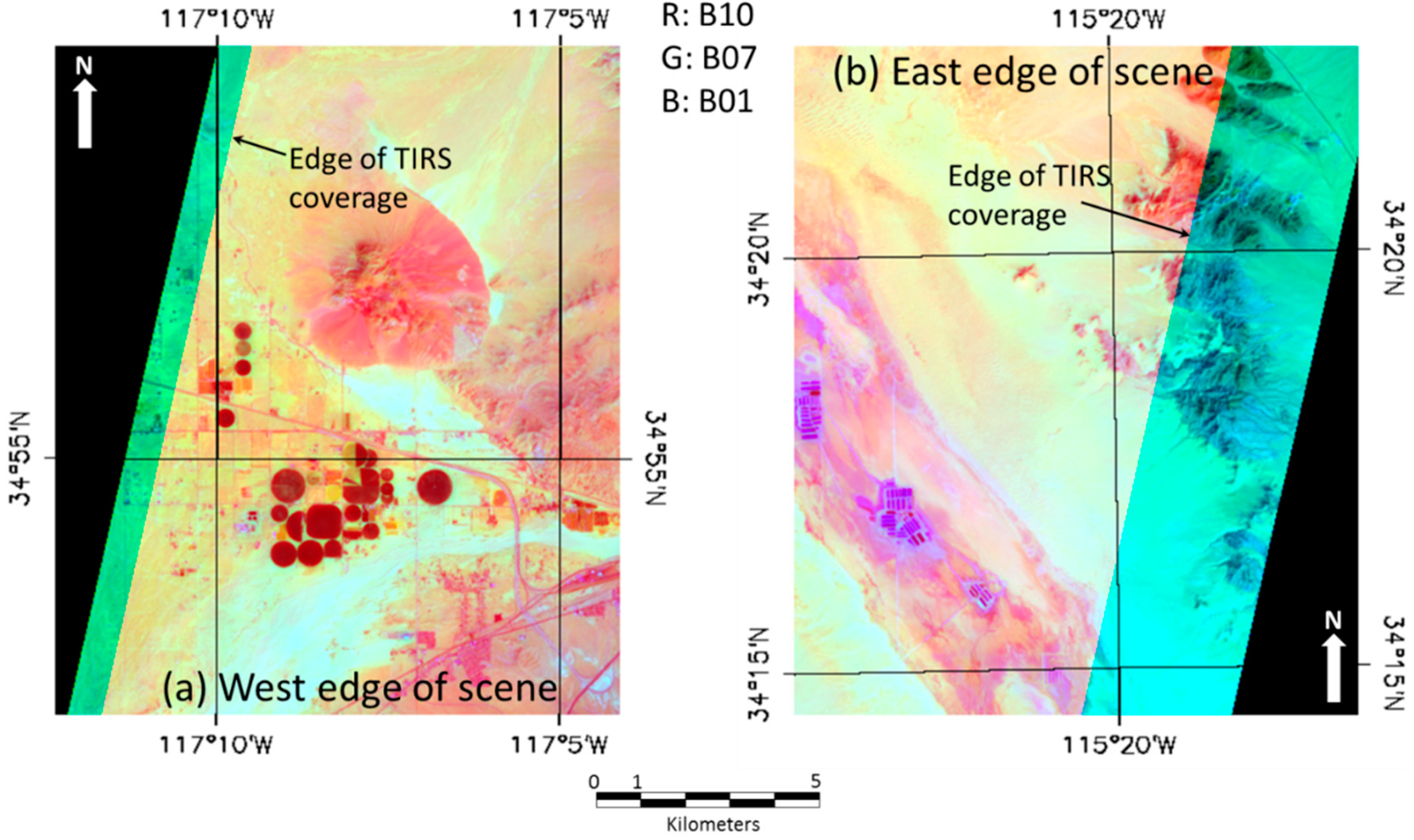
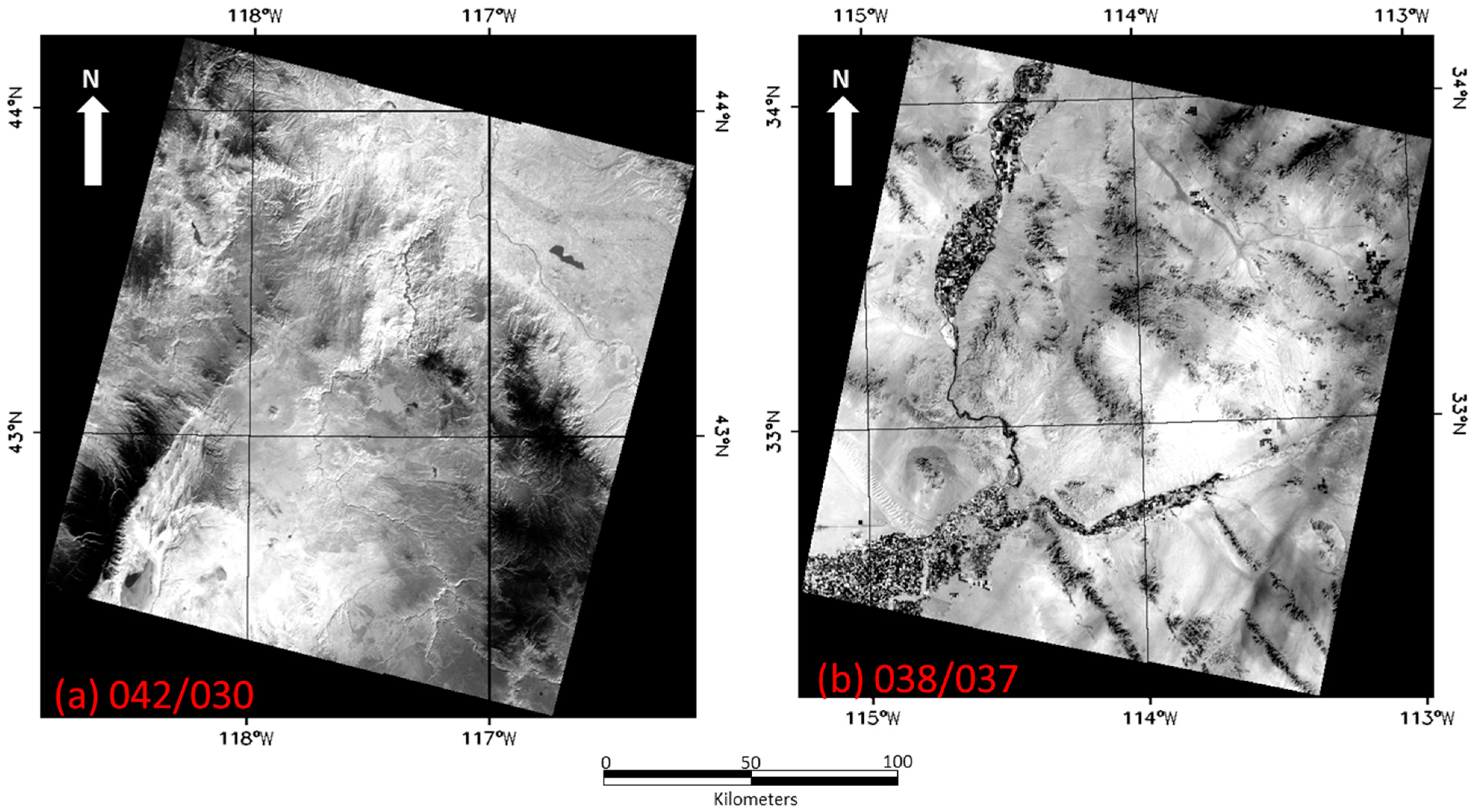
Cloud-free TIRS images over geometric calibration sites were then used to perform an initial quantitative update to the TIRS-to-spacecraft alignment. TIRS images over WRS path 042, row 030 from 9 March shown on the left side of Figure 8, and over WRS path 038, row 037 from 11 March shown on the right side of Figure 8, were used with Landsat 5 SWIR band reference images in the initial calibration. The coarse alignment updates made it possible to register the TIRS and GLS reference images sufficiently for the automated TIRS alignment calibration to operate. The TIRS alignment calibration procedure calculates corrections to both the TIRS-to-spacecraft and TIRS SCA-to-SCA alignments, and is described in the next section.

3.1. TIRS Alignment Calibration

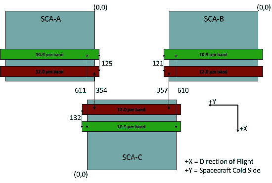
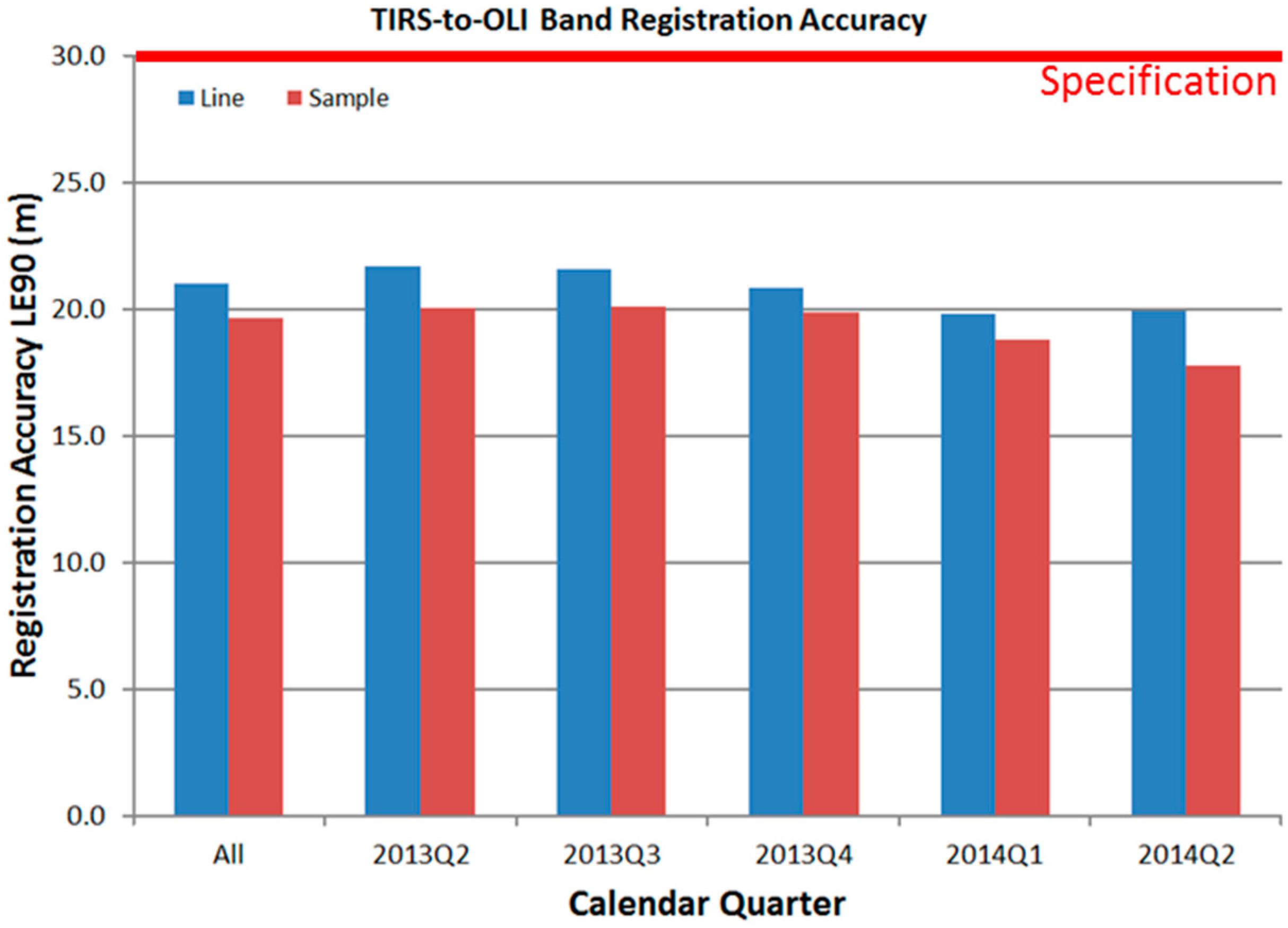
The on-orbit TIRS alignment calibration algorithm [7] was developed to simultaneously accomplish two objectives: (1) to measure TIRS-to-OLI instrument alignment, and (2) to detect and correct TIRS SCA-to-SCA misalignment. This is accomplished by generating Level 1T terrain and ground control point corrected TIRS images of the 10.9-micrometer band (band 10) in which each TIRS SCA is stored in its own output file. These SCA-separated images are then correlated with a Level 1T reference image created using the OLI SWIR1 (1610-nanometer) band (band 6). The measured image displacements from each SCA are used to estimate the overall alignment relationship between the TIRS and OLI instruments and to simultaneously correct any SCA-specific misalignments by adjusting the 8 Legendre coefficients that constitute each SCA’s line-of-sight model for the 10.9 micrometer band. The ultimate objective of this calibration is to ensure accurate registration between the TIRS and OLI spectral bands

Figure 8. Initial TIRS alignment calibration images, acquired prior to the first Operational Land Imager (OLI) imaging. (a) The interval on the left from WRS 042/030 acquired 9 March 2013 and (b) the interval on the right from WRS 038/037 acquired on 11 March 2013, provided the first complete TIRS on-orbit alignment calibration update, using Landsat 5 Thematic Mapper data as a reference.

Figure 8. Initial TIRS alignment calibration images, acquired prior to the first Operational Land Imager (OLI) imaging. (a) The interval on the left from WRS 042/030 acquired 9 March 2013 and (b) the interval on the right from WRS 038/037 acquired on 11 March 2013, provided the first complete TIRS on-orbit alignment calibration update, using Landsat 5 Thematic Mapper data as a reference.

Reliably matching data acquired by emissive (thermal) spectral bands with data from reflective spectral bands can be challenging due to the substantial differences in spectral response that are observed for many Earth targets. The ASTER mission was successful in operationally matching thermal bands to VNIR bands [10,11]. The approach used for TIRS relies on experience derived from Landsat 7 ETM+ data where it was found that the thermal and SWIR bands yielded the most consistent correlation performance [12].

The fundamental measurements used to perform the TIRS alignment calibration are TIRS-to-OLI image displacements measured at tie points in geometrically corrected Level 1T image space, using automated image correlation techniques. All of the TIRS geometric characterization and calibration algorithms utilize normalized gray scale correlation with a surface fitting polynomial to locate the peak of the correlation function to sub-pixel accuracy. This approach is similar to that used by ASTER [11] and ETM+ [12]. 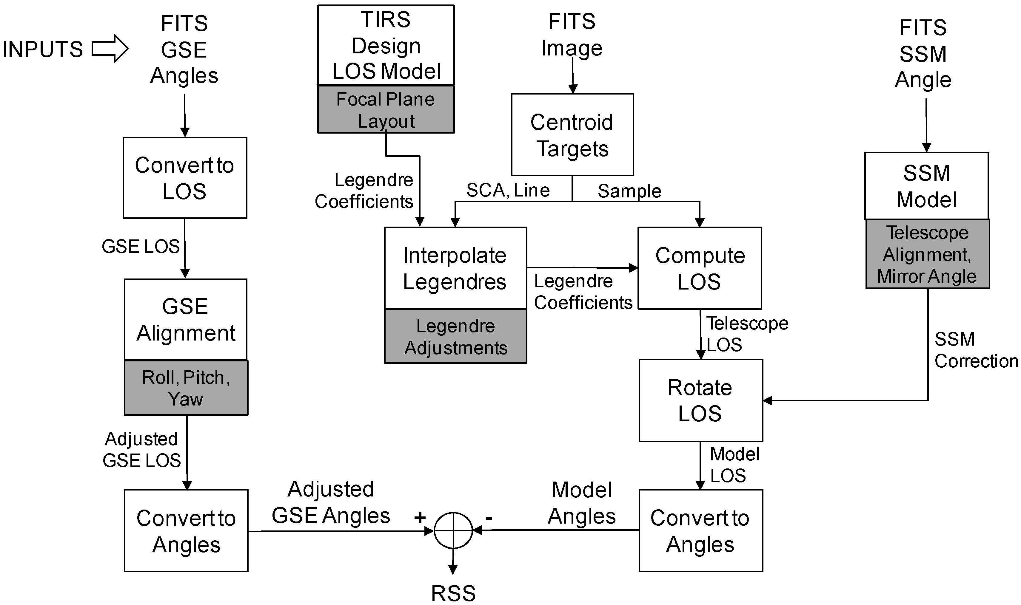When using well-defined image targets this method has been found to yield accuracy of 0.1 pixel or better [13]. The Level 1T row/column pixel coordinates of the original “search” TIRS tie point and of the corresponding “reference” location from the OLI image are both projected back into geometrically uncorrected TIRS line/detector image space using the TIRS geometric model. The detector coordinate is then used to compute a line-of-sight vector using the current Legendre coefficient model, per Equations (9) and (10). The search and reference line-of-sight vector coordinates and the search and reference line coordinates are differenced to compute apparent pointing offsets in the coordinate system used by the Legendre coefficient line-of-sight model:

$$X_{offset}=\frac{r_x}{r_z}-\frac{s_x}{s_z}+(reference line-search line)\times along track IFOV$$

(11)

$$Y_{offset}=\frac{r_y}{r_z}-\frac{s_y}{s_z}$$

(12)

where: $\left[\begin{array}{c}{r}_x\\ r_y\\ r_z\end{array}\right]$ and $\left[\begin{array}{c}{s}_x\\ s_y\\ s_z\end{array}\right]$ are the reference and search line-of-sight vectors, respectively.

Observations of this type for all three TIRS SCAs are used to simultaneously solve for 27 calibration parameter corrections: 3 TIRS-to-OLI alignment angles (roll-pitch-yaw) + (4 along-track 10.9 micrometer band Legendre coefficients + 4 cross-track 10.9 micrometer band Legendre coefficients) × 3 SCAs. Each X/Y observation pair contributes information to the three alignment angle corrections and to the 8 Legendre coefficient corrections for the SCA in which it was measured.

The alignment angle and Legendre coefficient corrections are highly correlated, so additional constraints are imposed on the fitting procedure to ensure that angular alignment adjustments are not absorbed by the Legendre polynomial model. These constraints are applied to the Legendre coefficient corrections to ensure that: (1) the sum of the cross-track corrections at the mid-points of the three SCAs is zero (suppressing roll effects); (2) the sum of the along-track corrections at the mid-points of the three SCAs is zero (suppressing pitch effects); and (3) the along-track corrections at the mid-points of the outboard SCAs are the same (suppressing yaw effects). Substituting a normalized detector coordinate of zero into equation (10) above shows that the adjustment to the X and Y line-of-sight coordinates for the center of an SCA can be constructed from the Legendre coefficient corrections as:

Δx_k = Δcoef_x_0k – Δcoef_x_2k / 2 (along-track)
Δy_k = Δcoef_y_0k – Δcoef_y_2k / 2 (cross-track)

(13)

where:

• Δcoef_x_0k and Δcoef_x_2k are the first and third x Legendre corrections for SCA k,
• Δcoef_y_0k and Δcoef_y_2k are the first and third y Legendre corrections for SCA k.

The constraint equations can thus be formulated as follows:

Δcoef_y₀₁ + Δcoef_y₀₂ + Δcoef_y₀₃ − (Δcoef_y₂₁ + Δcoef_y₂₂ + Δcoef_y₂₃)/2 = 0 (roll)
Δcoef_x₀₁ + Δcoef_x₀₂ + Δcoef_x₀₃ − (Δcoef_x₂₁ + Δcoef_x₂₂ + Δcoef_x₂₃)/2 = 0 (pitch)
Δcoef_x₀₁ − Δcoef_x₂₁/2 − Δcoef_x₀₃ + Δcoef_x₂₃ / 2 = 0 (yaw)

(14)

The collection of tie point measurements plus the three constraints are used in a least squares procedure to simultaneously estimate values for all 27 corrections. This solution procedure is iterated with a T-distribution outlier detection test that identifies and eliminates invalid tie point measurements. The final computed corrections are added to the current calibration parameters to create updated versions of the TIRS-to-OLI alignment and the Legendre coefficient line-of-sight model. The updated TIRS-to-OLI alignment matrix is then pre-multiplied by the OLI-to-spacecraft alignment matrix to construct the TIRS-to-spacecraft alignment matrix that is stored in the calibration parameter file (CPF) for operational use.

3.2. TIRS On-Orbit Alignment Calibration Operations

During the Landsat 8 commissioning period the first priority for geometric calibration was to refine the OLI geometric model [3]. Since the TIRS alignment calibration procedure uses OLI SWIR band imagery for its reference, a well calibrated OLI is a prerequisite for TIRS on-orbit calibration. Once well-calibrated OLI data were available, a series of 16 cloud-free scenes of geometric calibration sites, acquired between 21 March 2013, and 13 April 2013, were used to refine the TIRS alignment calibration. These calibration sites are arid regions, selected to provide a broad latitude distribution in both the northern and southern hemispheres, where Landsat 7 experience has shown that good SWIR band to thermal band correlation can be expected. It is important that clouds be avoided as the slight difference in along-track pointing direction of the TIRS and OLI detectors will introduce differences in the apparent locations of clouds that depend upon the cloud altitude. Clouds provide an extreme example of the parallax sensitivity that makes it necessary to terrain correct Landsat 8 image products to ensure proper instrument-to-instrument, SCA-to-SCA, and band-to-band alignment.

The measurements collected in the OLI/TIRS calibration scenes refined the initial TIRS alignment calibration derived from TIRS-only data to yield the first operational on-orbit calibration of the TIRS-to-OLI (and TIRS-to-spacecraft) alignment and the 10.9 micrometer band line-of-sight model. Table 5 shows the magnitude of the total TIRS instrument alignment and SCA placement adjustments applied to the prelaunch TIRS geometric model. Note that these adjustments include the effects of both the initial coarse corrections and the subsequent results from the TIRS alignment calibration procedure.

Table 5. On-orbit estimate of TIRS-to-spacecraft alignment, changes from the prelaunch alignment, and SCA placement updates resulting from Legendre coefficient model refinement. The alignment results show that the prelaunch TIRS alignment measurement met the TIRS alignment knowledge requirement of 2 milliradians (3 σ) [9]. Note the large adjustment to the cross-track position of SCA-A.

Parameter		Roll (Milliradians)	Pitch (Milliradians)		Yaw (Milliradians)
On-Orbit TIRS-to-Spacecraft Alignment		0.197	2.148		2.265
Change from Prelaunch Alignment		−1.576	1.447		0.521
SCA	Along-Track Offset (Microradians)			Cross-Track Offset (Microradians)
A	−49			−753
B	−77			−102
C	156			77

Table 5. On-orbit estimate of TIRS-to-spacecraft alignment, changes from the prelaunch alignment, and SCA placement updates resulting from Legendre coefficient model refinement. The alignment results show that the prelaunch TIRS alignment measurement met the TIRS alignment knowledge requirement of 2 milliradians (3 σ) [9]. Note the large adjustment to the cross-track position of SCA-A.

Parameter		Roll (Milliradians)	Pitch (Milliradians)		Yaw (Milliradians)
On-Orbit TIRS-to-Spacecraft Alignment		0.197	2.148		2.265
Change from Prelaunch Alignment		−1.576	1.447		0.521
SCA	Along-Track Offset (Microradians)			Cross-Track Offset (Microradians)
A	−49			−753
B	−77			−102
C	156			77

Noting that the TIRS pixel dimension is 142 microradians, the magnitude of the SCA-A cross-track adjustment can be seen to be more than 5 pixels. The sign of this adjustment is such that it counteracts the approximately 3.5-pixel adjustment applied as a result of the prelaunch TVAC measurements. The other SCA placement adjustments are on the order of one TIRS pixel or less, but they are larger than expected based upon the prelaunch calibration results. A loss of index in the steering mirror position telemetry during TVAC testing is suspected as the source of the anomalous cross-track error in prelaunch position for SCA-A.

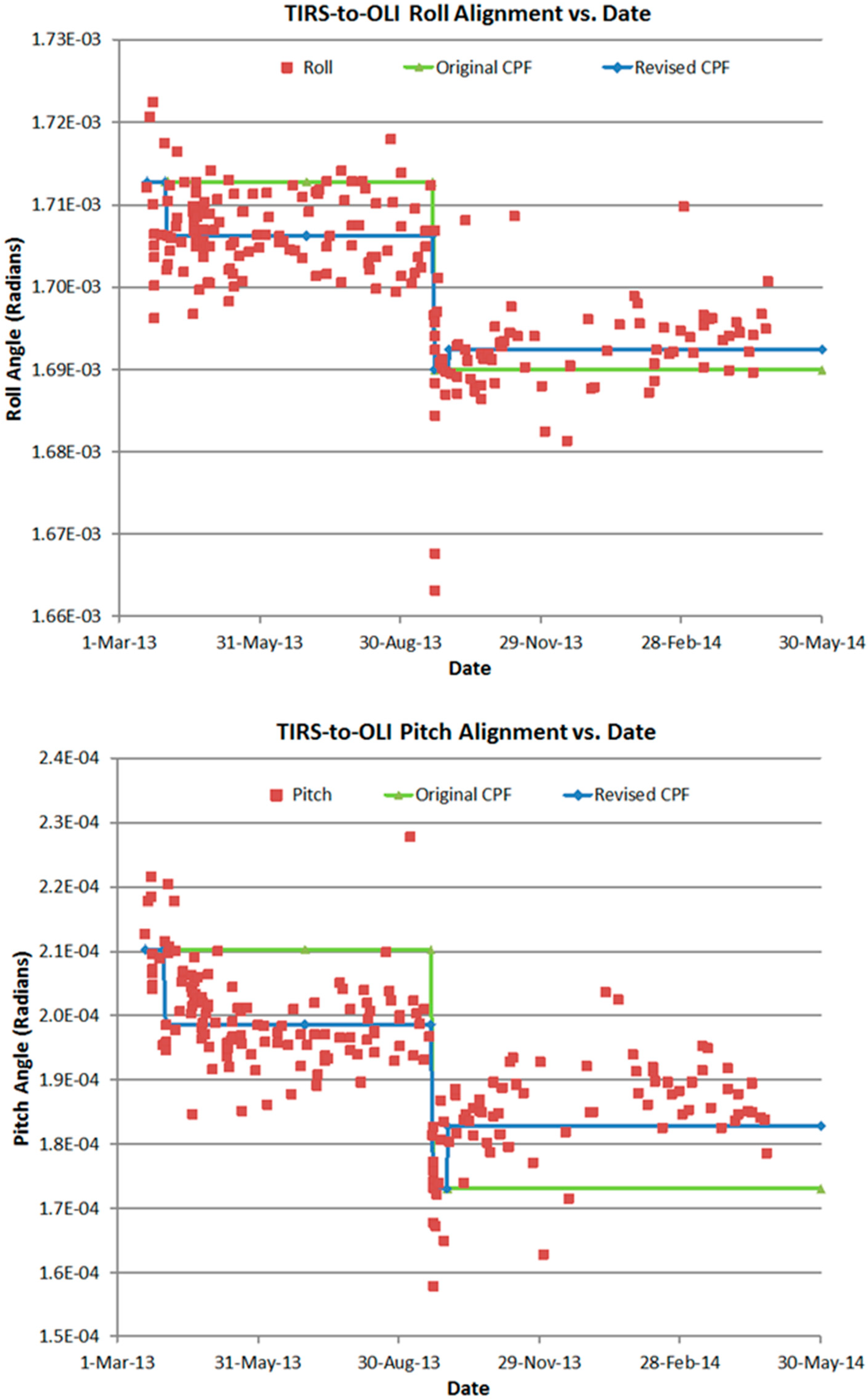
Figure 9. TIRS-to-OLI (a) roll (top) and (b) pitch (bottom) alignment measurements over time show a step discontinuity at the spacecraft safe-hold anomaly that occurred in late-September 2013. An update to the alignment calibration was issued shortly after imaging operations resumed (green lines). The entire calibration time history was subsequently refined (blue lines) in preparation for the February 2014 data reprocessing campaign.

Figure 9. TIRS-to-OLI (a) roll (top) and (b) pitch (bottom) alignment measurements over time show a step discontinuity at the spacecraft safe-hold anomaly that occurred in late-September 2013. An update to the alignment calibration was issued shortly after imaging operations resumed (green lines). The entire calibration time history was subsequently refined (blue lines) in preparation for the February 2014 data reprocessing campaign.

TIRS alignment calibration operations continue to be performed routinely to ensure that TIRS/OLI registration accuracy is maintained. These measurements have captured several changes in TIRS alignment behavior that have led to additional on-orbit adjustments to the TIRS-to-spacecraft alignment calibration. No significant changes to TIRS Legendre coefficient line-of-sight model have been observed. Figure 9 shows the time history of TIRS-to-OLI roll and pitch alignment measurements through the first quarter of 2014. Changes in this relationship, as distinct from common changes in the alignment of the two instruments to the spacecraft, can lead to errors in emissive-to-reflective band registration.

Figure 9 shows an abrupt change in apparent alignment in September 2013. This change was associated with an attitude control anomaly and resulting spacecraft safe-hold event that led to significant changes in the temperature environment around the instrument deck. Once imaging operations resumed following this event the TIRS alignment was checked and found to be more than 30 microradians different than the then-current calibrated value in the pitch axis. A smaller roll axis change was observed. The anomalous data points in this area are a result of using less-than-ideal scenes to make alignment measurements in the immediate aftermath of the anomaly.

An immediate update to the TIRS alignment calibration was issued to compensate for the observed change. The green lines on Figure 9 show the calibrated values. The TIRS alignment appeared to partially recover towards its previous condition in the weeks following the anomaly. This motivated an additional calibration update effective on 1 October 2013. When the decision was made to reprocess the entire Landsat 8 data set, in order to implement a significant improvement to the radiometric calibration knowledge, an additional refinement to the TIRS alignment calibration time history was implemented to better capture the changes in behavior that occurred during the commissioning period as the spacecraft was being maneuvered into its operational orbit. This change is most easily seen in the pitch axis where there is a declining trend in the early data. An additional source of variation affecting the early commissioning data that were acquired prior to achieving the operational WRS-2 orbit was a series of adjustments to the control temperatures for the TIRS telescope. The TIRS instrument team made these adjustments as part of the process of achieving best focus for the TIRS instrument.

The revised calibration, shown by the blue lines in Figure 9, was used during the data reprocessing campaign conducted in February 2014, and is the basis for the performance results reported below. Table 6 shows the current best estimates of the TIRS-to-OLI alignment angles and the magnitudes of the adjustments that have been made over time.

Table 6. TIRS-to-OLI alignment calibration angles over time are shown along with the magnitude of the adjustments that have been applied.

Time Period	Roll Angle (Micro-radians)	Roll Change (Micro-radians)	Pitch Angle (Micro-radians)	Pitch Change (Micro-radians)	Yaw Angle (Micro-radians)	Yaw Change (Micro-radians)
Launch–31MAR2013	1713	-	210	-	2753	-
01APR2013–20SEP2013	1706	−6	199	−12	2770	16
21SEP2013–30SEP2013	1690	−16	173	−25	2775	5
01OCT2013–30SEP2014	1692	2	183	10	2761	−14

Table 6. TIRS-to-OLI alignment calibration angles over time are shown along with the magnitude of the adjustments that have been applied.

Time Period	Roll Angle (Micro-radians)	Roll Change (Micro-radians)	Pitch Angle (Micro-radians)	Pitch Change (Micro-radians)	Yaw Angle (Micro-radians)	Yaw Change (Micro-radians)
Launch–31MAR2013	1713	-	210	-	2753	-
01APR2013–20SEP2013	1706	−6	199	−12	2770	16
21SEP2013–30SEP2013	1690	−16	173	−25	2775	5
01OCT2013–30SEP2014	1692	2	183	10	2761	−14

The largest alignment adjustments shown in Table 6 are associated with the late-September 2013 spacecraft safe-hold event described above. A more recent spacecraft safe-hold did not lead to a similar alignment disruption due to more careful management of the on-board heaters, and resulting temperatures, during the event. This was a lesson learned from the first anomaly. The apparent sensitivity of TIRS alignment to the temperature environment was not unexpected as prelaunch thermal/mechanical analysis had predicted that measureable within-orbit thermally induced changes in TIRS pointing might be expected [8]. Though some evidence of a latitude-dependent alignment effect has been observed, it is within the allowable instrument alignment stability thresholds so a position-in-orbit based alignment model has not been attempted and is not currently contemplated. The within-orbit effect as well as the potential for seasonal thermal effects motivates continued careful monitoring. Additional alignment updates will continue to be issued as events dictate.

3.3. TIRS Band Alignment Calibration

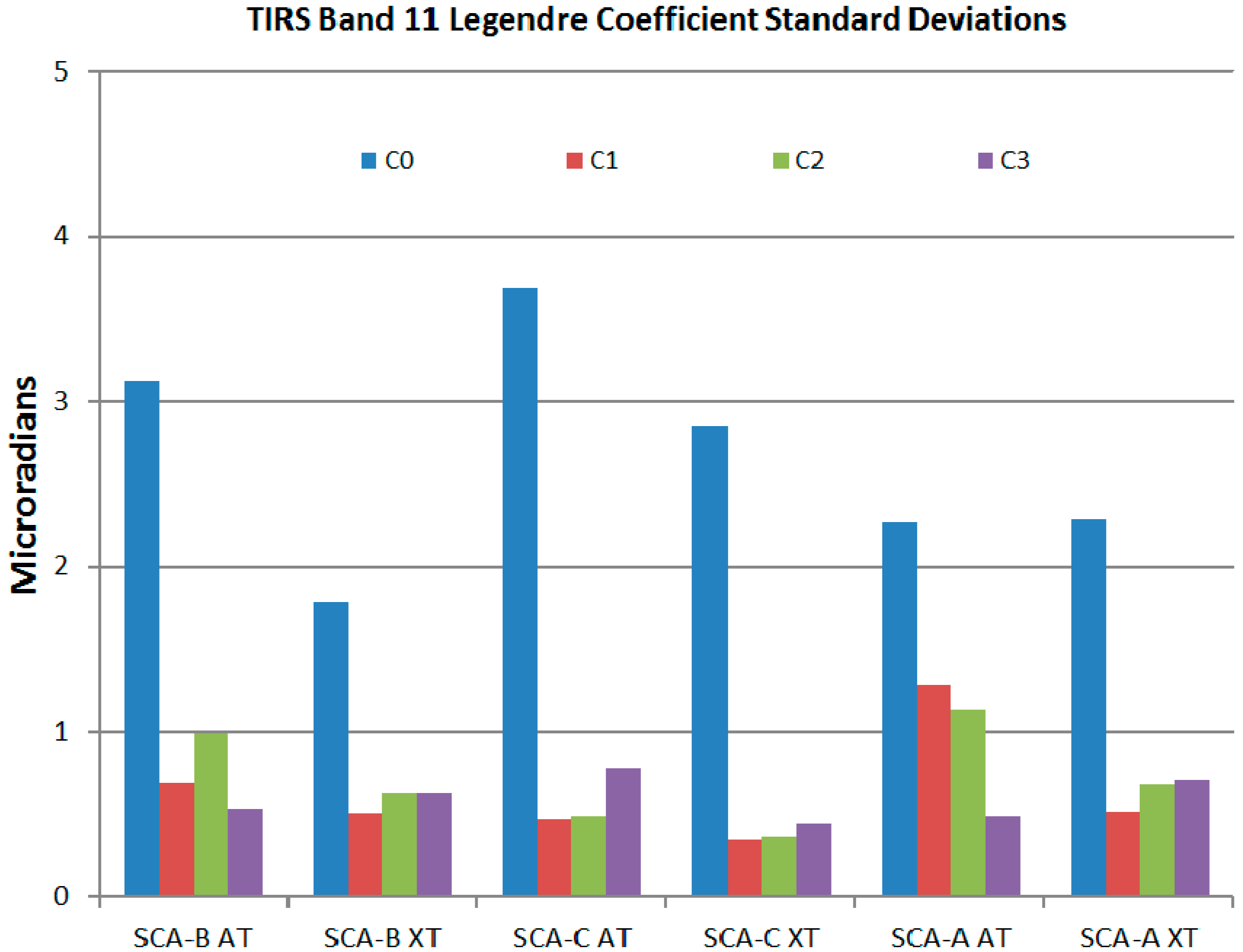
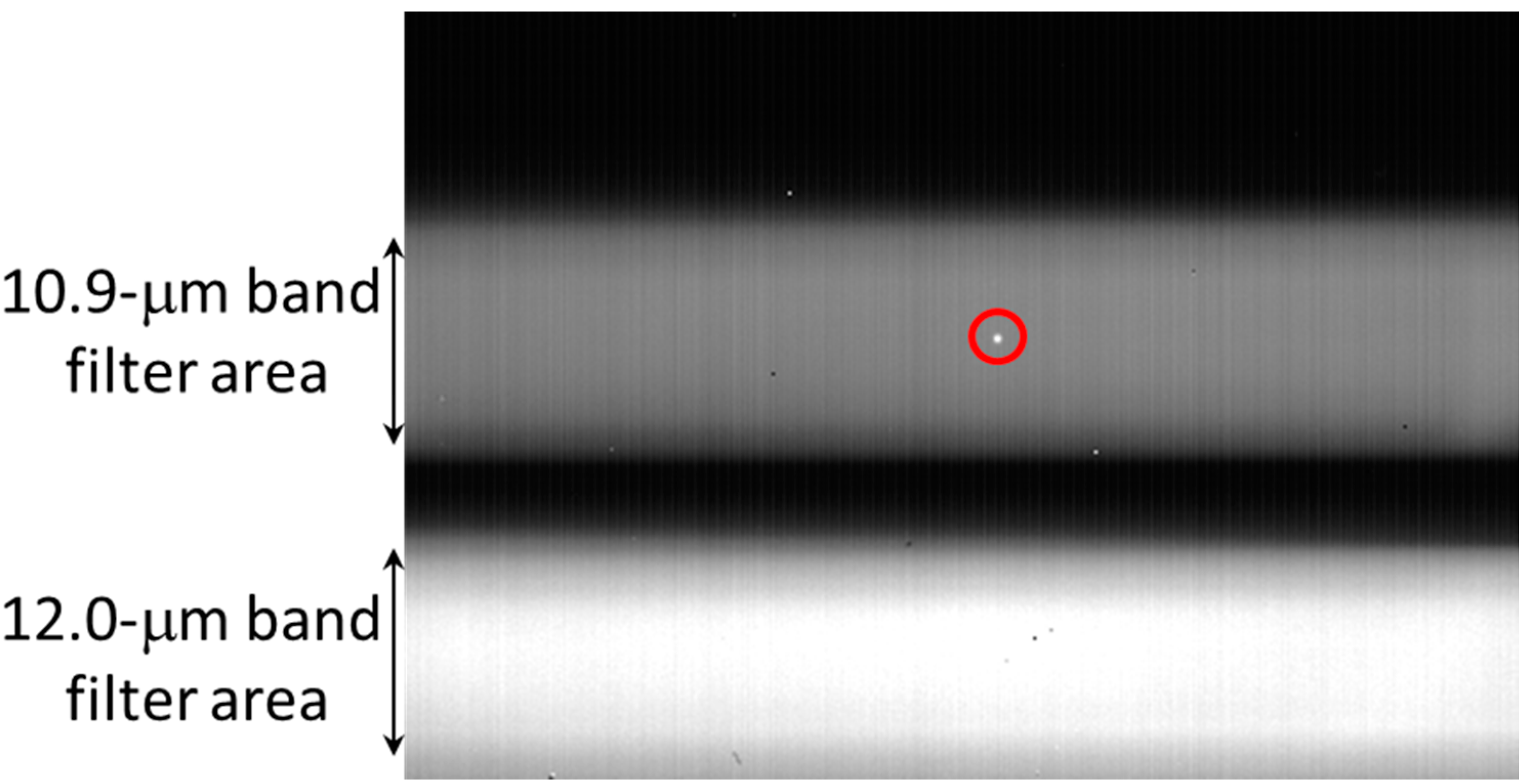
As described above, the TIRS alignment calibration procedure is used to refine both the overall TIRS-to-OLI alignment knowledge and the Legendre polynomial operational line-of-sight model coefficients for the 10.9-micrometer band (band 10) on each individual TIRS SCA. Having updated the pointing model for band 10, the alignment of the TIRS 12.0-micrometer band (band 11) to band 10 must be updated to restore TIRS internal band-to-band consistency. The TIRS band alignment calibration process uses SCA-separated images containing both TIRS spectral bands to measure band-to-band tie points with band 10 serving as the reference for band 11. The spectral similarity of the two bands makes this a relatively straightforward process with little sensitivity to scene content, other than the necessity of avoiding clouds. A set of ten cloud-free calibration scenes over desert sites, a subset of those used for TIRS alignment calibration, was used for on-orbit TIRS band alignment calibration. As was the case for TIRS alignment, tie point offsets measured in Level 1T image space are converted to the corresponding uncorrected detector/line coordinates and then to along-track and cross-track angular displacements using Equations (11) and (12). The preprocessed tie point measurements from each SCA are then used in a least squares solution to compute updates to the eight band 11 Legendre coefficients for that SCA. The Legendre coefficient updates for the calibration scenes were averaged to generate the final on-orbit update to the band 11 line-of-sight model.

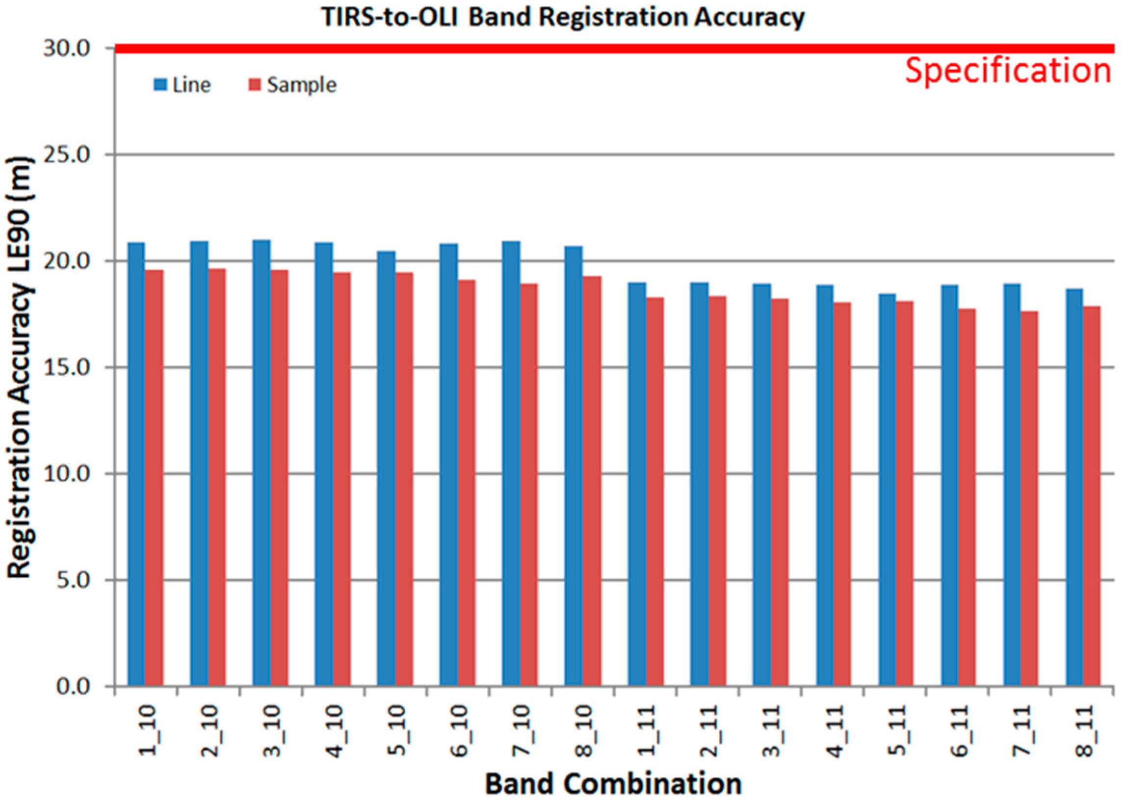
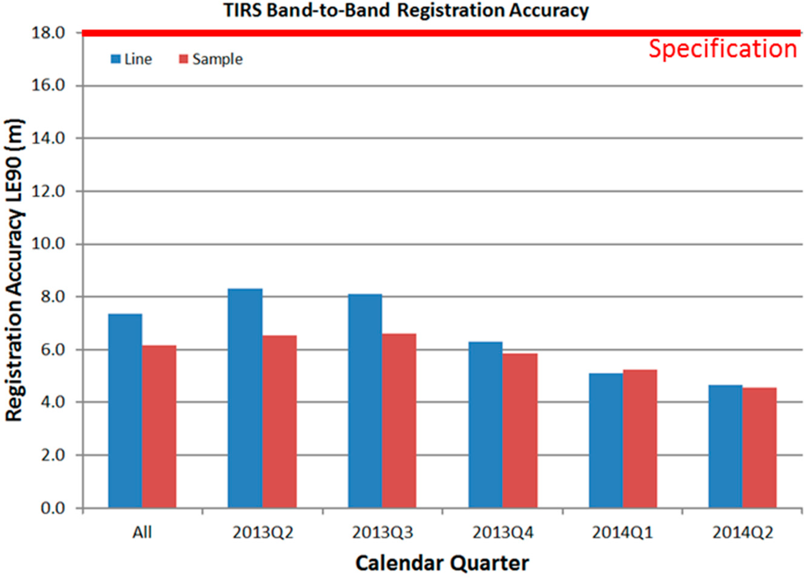
The standard deviations of the calculated Legendre coefficient updates are shown in Figure 10. Converting the standard deviations to 90% linear error (LE90) and summing the contributions from the four coefficients for each direction and SCA yields a maximum uncertainty less than 6.4 meters in the along-track direction and less than 4.9 meters in the cross-track direction. Calibration error should thus contribute only a small amount to the 18-meter (LE90) TIRS band registration performance requirement.

4. TIRS On-Orbit Geometric Performance Characterization

In addition to meeting the geometric accuracy requirements listed in Table 1 and the TIRS-to-spacecraft alignment knowledge requirement noted in Table 5, the TIRS instrument was required to be absolutely aligned to the spacecraft to within 5 milliradians (3σ) in each axis [9] to ensure co-alignment between the OLI and TIRS instrument fields of view. The on-orbit TIRS-to-spacecraft alignment angle measurements shown in Table 5 are all well below 5 milliradians, demonstrating that the required alignment control was achieved. Figure 11 shows an OLI-TIRS color composite image pair that demonstrates the relationship between the OLI and TIRS instrument fields of view. The two image windows were extracted from the western and eastern edges of a scene and show that the TIRS field of view (red image channel) is completely contained within the OLI field of view (green and blue channels) providing coincident reflective band coverage for the full thermal band swath.

Figure 10. Standard deviations of band 11 (12.0-μm) to band 10 (10.9-μm) band alignment calibration Legendre coefficient updates in the X/along-track (AT) and Y/cross-track (XT) directions. All SCAs showed good consistency (better than 4 microradians) relative to the 142-microradian TIRS pixel size.

Figure 10. Standard deviations of band 11 (12.0-μm) to band 10 (10.9-μm) band alignment calibration Legendre coefficient updates in the X/along-track (AT) and Y/cross-track (XT) directions. All SCAs showed good consistency (better than 4 microradians) relative to the 142-microradian TIRS pixel size.

Figure 11. OLI-TIRS composite image with the TIRS 10.9-micrometer band (band 10) in the red channel, the OLI SWIR2 band (band 7) in the green channel, and the OLI coastal-aerosol band (band 1) in the blue channel. (a) The left image window was extracted from the western edge of the scene and (b) the right window was extracted from the eastern edge of the scene. Note that the TIRS coverage is contained within the OLI coverage.

Figure 11. OLI-TIRS composite image with the TIRS 10.9-micrometer band (band 10) in the red channel, the OLI SWIR2 band (band 7) in the green channel, and the OLI coastal-aerosol band (band 1) in the blue channel. (a) The left image window was extracted from the western edge of the scene and (b) the right window was extracted from the eastern edge of the scene. Note that the TIRS coverage is contained within the OLI coverage.

As described in Section 3, the TIRS geometric calibration strategy is based upon aligning the TIRS 10.9-micrometer band to the OLI and then aligning the TIRS 12.0-micrometer band to the 10.9-micrometer band. By sharing a common spacecraft/platform model, absolute geodetic (geolocation) and geometric (Level 1T product) accuracy are transferred from the OLI to the TIRS making it unnecessary to, for example, measure ground control points in the TIRS imagery. TIRS-to-OLI registration accuracy and TIRS band-to-band registration accuracy are thus the fundamental aspects of TIRS geometric performance that are verified by direct measurement. Geodetic and geometric accuracy are inferred from the measured OLI performance [3] as described in Section 4.3.

4.1. TIRS-to-OLI Band Registration Accuracy

SCA-by-SCA tie point measurements between TIRS band 10 (10.9-micrometer) and OLI band 6 (SWIR1) are part of the TIRS alignment calibration procedure described above. Full band (combined SCA) measurements are also made between each TIRS spectral band and all OLI bands, except the cirrus band, in order to determine the resulting TIRS emissive to OLI reflective band registration accuracy. These measurements are made using scenes over the same arid test sites used for TIRS alignment calibration to provide good band-to-band image correlation performance. Summary results, expressed as LE90 registration in the line and sample directions for the first 13 months of operation for every TIRS/OLI band combination are shown in Figure 12. Note that the results for TIRS band 11 (12.0-micrometer) are somewhat better than those for TIRS band 10. Band 11 is closer to nadir, and closer to the OLI field of view, in the along-track direction than is band 10. This makes band 11 less sensitive to terrain parallax effects.

Figure 12. TIRS emissive to OLI reflective band LE90 registration (in meters) in the line and sample directions. Summary results for every TIRS-to-OLI band combination. The 30-meter LE90 registration accuracy requirement is shown by the red line.

Figure 12. TIRS emissive to OLI reflective band LE90 registration (in meters) in the line and sample directions. Summary results for every TIRS-to-OLI band combination. The 30-meter LE90 registration accuracy requirement is shown by the red line.

There is no substantial variation in registration performance across the OLI bands, suggesting that correlation performance variability across the different band combinations is not playing a significant role in the final results. Performance in the sample direction is slightly better than the line direction. This is attributed to the somewhat higher degree of TIRS-to-OLI alignment variability observed in the pitch direction as compared to the roll direction.

The worst-case band combination registration results for each calendar quarter are shown in Figure 13. Recent performance has been slightly better than that observed over the first several quarters of operations. This is likely due to better TIRS alignment calibration in the absence of significant temperature anomalies since late 2013.

Figure 13. TIRS emissive to OLI reflective band LE90 registration (in meters) in the line and sample directions. Worst-case band combination results by calendar quarter. The 30-meter LE90 registration accuracy requirement is shown by the red line.

Figure 13. TIRS emissive to OLI reflective band LE90 registration (in meters) in the line and sample directions. Worst-case band combination results by calendar quarter. The 30-meter LE90 registration accuracy requirement is shown by the red line.

The overall TIRS-to-OLI band registration accuracy results for the worst-case band pair measured using data acquired between April 2013 and May 2014 are shown in Table 7.

Table 7. TIRS-to-OLI and TIRS band-to-band LE90 registration accuracy performance in meters, in the line and sample directions, are shown along with the associated requirement thresholds.

Registration Accuracy	Line Direction	Sample Direction	Requirement
TIRS emissive to OLI reflective	21.0 meters	19.6 meters	30 meters
10.9-µm to 12.0-µm	7.4 meters	6.2 meters	18 meters

Table 7. TIRS-to-OLI and TIRS band-to-band LE90 registration accuracy performance in meters, in the line and sample directions, are shown along with the associated requirement thresholds.

Registration Accuracy	Line Direction	Sample Direction	Requirement
TIRS emissive to OLI reflective	21.0 meters	19.6 meters	30 meters
10.9-µm to 12.0-µm	7.4 meters	6.2 meters	18 meters

4.2. TIRS Band-to-Band Registration Accuracy

As was the case for TIRS-to-OLI registration, in addition to the SCA-by-SCA tie point measurements used for TIRS band alignment calibration, full scene (SCA combined) measurements are collected to characterize the resulting band registration accuracy. Due to the spectral similarity of the two TIRS bands, scene content is less important in this case as compared to TIRS-to-OLI registration. Table 7 shows the summary measured TIRS band-to-band registration accuracy for the time period from April 2013 through May 2014.

Figure 14 shows the measured LE90 thermal band-to-band registration accuracy in the line and sample directions by calendar quarter. The superior performance of the more recent data is attributed to the more stable thermal environment resulting from the lack of anomalous events since late 2013.

Figure 14. TIRS 10.9-micrometer band to 12.0-micrometer band LE90 registration (in meters) in the line and sample directions by calendar quarter. The 18-meter LE90 registration accuracy requirement is shown by the red line.

Figure 14. TIRS 10.9-micrometer band to 12.0-micrometer band LE90 registration (in meters) in the line and sample directions by calendar quarter. The 18-meter LE90 registration accuracy requirement is shown by the red line.

4.3. Geometric Performance Propagated from OLI

Absolute geodetic accuracy refers to the geolocation accuracy of a geometrically corrected image prior to the application of ground control points, i.e., the accuracy achievable using only spacecraft navigation information. Geometric accuracy refers to the horizontal positional accuracy of a Level 1T image product, corrected using ground control points and digital elevation data. As mentioned above, the absolute geodetic accuracy and geometric accuracy items listed in Table 1 are not measured directly but rather are derived from the corresponding measured OLI performance and the TIRS-to-OLI registration accuracy. Since the TIRS-to-OLI registration performance stated in Table 7 is for the worst-case band combination, it can be combined with the published OLI geodetic and geometric accuracy results [3] to estimate worst-case TIRS performance. The only minor complication in this process is the need to convert the LE90 TIRS-to-OLI registration accuracy to a CE90 equivalent for compatibility with the two-dimensional geodetic accuracy and geometric accuracy requirements. This is done by taking the larger of the line and sample LE90 accuracy results, dividing by 1.6449 to convert to 1σ accuracy, and then multiplying by 2.146 to convert to CE90. Note that these manipulations presume that the errors represented by these accuracy estimates are Gaussian. The propagated TIRS performance is computed as the root-sum-square of the measured OLI performance and the (CE90 equivalent) TIRS-to-OLI registration accuracy. The results of these calculations are shown in Table 8 along with the corresponding TIRS accuracy requirements, repeated from Table 1. The estimated TIRS performance is well within the requirement limits in both cases.

Table 8. Propagated estimates of TIRS absolute geodetic (geolocation) accuracy and geometric (Level 1T product) accuracy are derived from measured OLI performance [3] and TIRS-to-OLI registration accuracy.

Metric	Measured OLI Performance (CE90) [3]	TIRS-to-OLI Registration as CE90	Propagated TIRS Performance (CE90)	Requirement Threshold (CE90)
Geodetic Accuracy	18.1 meters (global estimate)	27.4 meters	32.8 meters	76 meters
Geometric Accuracy	11.7 meters (GLS anchor sites)	27.4 meters	29.8 meters	42 meters

Table 8. Propagated estimates of TIRS absolute geodetic (geolocation) accuracy and geometric (Level 1T product) accuracy are derived from measured OLI performance [3] and TIRS-to-OLI registration accuracy.

Metric	Measured OLI Performance (CE90) [3]	TIRS-to-OLI Registration as CE90	Propagated TIRS Performance (CE90)	Requirement Threshold (CE90)
Geodetic Accuracy	18.1 meters (global estimate)	27.4 meters	32.8 meters	76 meters
Geometric Accuracy	11.7 meters (GLS anchor sites)	27.4 meters	29.8 meters	42 meters

4.4. TIRS Image Registration Accuracy

The final element of TIRS geometric performance is multi-temporal image-to-image registration accuracy. This aspect of TIRS geometric performance is directly measured but is not considered to be a stressing requirement and is therefore not assessed with the same frequency as the other performance characteristics. TIRS image-to-image registration accuracy is measured by correlating a dense array of tie points in the 10.9-micrometer band images from two Level 1T products over the same site acquired on different dates. Table 9 shows the registration results for 240 scene-pairs acquired over the first 14 months of operations.

Table 9. TIRS image registration accuracy is measured by correlating dense arrays of tie points in the 10.9-micrometer band for images of the same site acquired at different times. Summary results for 240 scene-pairs are shown as LE90 accuracy in meters.

Metric	Line Direction	Sample Direction	Requirement
Image Registration Accuracy	21.7 meters	16.3 meters	45 meters

Table 9. TIRS image registration accuracy is measured by correlating dense arrays of tie points in the 10.9-micrometer band for images of the same site acquired at different times. Summary results for 240 scene-pairs are shown as LE90 accuracy in meters.

Metric	Line Direction	Sample Direction	Requirement
Image Registration Accuracy	21.7 meters	16.3 meters	45 meters

Since Level 1T products are registered to the GLS ground control framework using the OLI reflective bands, TIRS multi-temporal image registration accuracy will be, to some degree, dependent upon the stability of TIRS-to-OLI registration. The fact that the TIRS image registration accuracy is slightly better than the TIRS-to-OLI registration accuracy suggests that a significant portion of the TIRS-to-OLI registration variability presented in Table 7 is due to effects, such as thermally induced within-orbit alignment changes, that are repeatable for a given ground location. Some of the TIRS-to-OLI registration error thus cancels out when comparing two TIRS images over the same site.

5. Summary and Conclusions

Following its launch in February 2013, the Landsat 8 TIRS instrument entered a commissioning period that included an intensive set of on-orbit geometric calibration procedures. This calibration activity measured the alignment of the TIRS instrument relative to the OLI instrument, refined the prelaunch knowledge of the relative locations of the three TIRS sensor chips assemblies (SCAs), and aligned the 12.0-micrometer spectral band to the 10.9-micrometer band. The initial instrument alignment checks showed that good TIRS-to-OLI field of view co-alignment was achieved during spacecraft integration. The unexpectedly large magnitudes of some of the required adjustments to the prelaunch TIRS line-of-sight model parameters indicated that the challenging prelaunch calibration measurement campaign was only partially successful in establishing an accurate baseline geometric model. Fortunately, TIRS has been shown to meet all geometric requirements using the results of the on-orbit geometric calibration for geometric correction processing. Key performance results, compared to the corresponding mission requirements, are summarized in Table 10.

The geometric calibration of the TIRS instrument continues to be monitored and updated as necessary to maintain performance. On-board events that disturb the instrument’s thermal environment, specifically a spacecraft anomaly that occurred in September 2013, have been shown to disrupt the TIRS alignment sufficiently to require recalibration. Some evidence of the within-orbit alignment variability predicted by the prelaunch STOP model has been observed on-orbit, but with a smaller magnitude than was predicted. The potential for longer-term, possibly seasonal, sensitivity to the on-orbit thermal environment is a focus of the on-going calibration activity to monitor and update the TIRS line-of-sight model.

Table 10. Using the line-of-sight model parameters determined through on-orbit geometric calibration, the TIRS instrument is meeting all geometric performance requirements. Key performance characteristics and the corresponding requirements are shown for comparison.

Characteristic	TIRS Performance	Requirement
TIRS-to-Spacecraft Alignment Accuracy	2.3 milliradians (worst axis)	5 milliradians (3-sigma)
TIRS-to-Spacecraft Alignment Knowledge (Prelaunch)	1.6 milliradians (worst axis)	2 milliradians (3-sigma)
TIRS Field-of-View (Swath)	186.2 kilometers	185 kilometers
TIRS-to-OLI Registration Accuracy	21.0 meters (LE90) (worst direction)	30 meters (LE90)
TIRS Band-to-Band Registration Accuracy	7.4 meters (LE90) (worst direction)	18 meters (LE90)
TIRS Absolute Geodetic Accuracy	32.7 meters (CE90)	76 meters (CE90)
TIRS Geometric (Level 1T Product) Accuracy	29.8 meters (CE90)	42 meters (CE90)
TIRS Image Registration Accuracy	21.7 meters (LE90) (worst direction)	45 meters (LE90)

Table 10. Using the line-of-sight model parameters determined through on-orbit geometric calibration, the TIRS instrument is meeting all geometric performance requirements. Key performance characteristics and the corresponding requirements are shown for comparison.

Characteristic	TIRS Performance	Requirement
TIRS-to-Spacecraft Alignment Accuracy	2.3 milliradians (worst axis)	5 milliradians (3-sigma)
TIRS-to-Spacecraft Alignment Knowledge (Prelaunch)	1.6 milliradians (worst axis)	2 milliradians (3-sigma)
TIRS Field-of-View (Swath)	186.2 kilometers	185 kilometers
TIRS-to-OLI Registration Accuracy	21.0 meters (LE90) (worst direction)	30 meters (LE90)
TIRS Band-to-Band Registration Accuracy	7.4 meters (LE90) (worst direction)	18 meters (LE90)
TIRS Absolute Geodetic Accuracy	32.7 meters (CE90)	76 meters (CE90)
TIRS Geometric (Level 1T Product) Accuracy	29.8 meters (CE90)	42 meters (CE90)
TIRS Image Registration Accuracy	21.7 meters (LE90) (worst direction)	45 meters (LE90)

References and Notes

1. Irons, J.; Dwyer, J.; Barsi, J. The next Landsat satellite: The Landsat data continuity mission. Remote Sens. Environ. 2012, 122, 11–21. [Google Scholar] [CrossRef]
2. Knight, E.; Kvaran, G. Landsat-8 operational land imager design, characterization, and performance. Remote Sens. 2014, 6, 10286–10305. [Google Scholar] [CrossRef]
3. Storey, J.; Choate, M.; Lee, K. Landsat-8 operational land imager on-orbit geometric calibration and performance. Remote Sens. 2014, in press. [Google Scholar]
4. Reuter, D.; Richardson, C.; Pellerano, F.; Irons, J.; Allen, R.; Anderson, M.; Jhabvala, M.; Lunsford, A.; Montanaro, M.; Smith, R.; et al. The Thermal Infrared Sensor (TIRS) on Landsat 8: Design overview and pre-launch characterization. Remote Sens. 2014. under review. [Google Scholar]
5. NASA. Landsat Data Continuity Mission Thermal Infrared Sensor Requirements Document—Revision F1; NASA Goddard Space Flight Center: Greenbelt, MD, USA, 2012. [Google Scholar]
6. ZEMAX EE. Software for Optical System Design, ZEMAX Development Corporation. Available online: http://www.zemax.com/ (accessed on 10 October 2014).
7. USGS. LDCM Cal/Val Algorithm Description Document—Version 3.0; U.S. Geological Survey: Sioux Falls, SD, USA, 2013. [Google Scholar]
8. Cheng, K. Final TIRS Structural Thermal Optical Performance (STOP) Analysis Report; NASA Goddard Space Flight Center: Greenbelt, MD, USA, 2011. [Google Scholar]
9. NASA. Landsat Data Continuity Mission Observatory Interface Requirements Document—Revision D6; NASA Goddard Space Flight Center: Greenbelt, MD, USA, 2009. [Google Scholar]
10. Fujisada, H. ASTER Level-1 data processing algorithm. IEEE Trans. Geosci. Remote Sens. 1998, 36, 1101–1112. [Google Scholar] [CrossRef]
11. Iwasaki, A.; Fujisada, H. ASTER geometric performance. IEEE Trans. Geosci. Remote Sens. 2005, 43, 2700–2706. [Google Scholar] [CrossRef]
12. Lee, D.; Storey, J.; Choate, M.; Hayes, R. Four years of Landsat-7 on-orbit geometric calibration and performance. IEEE Trans. Geosci. Remote Sens. 2004, 42, 2786–2795. [Google Scholar] [CrossRef]
13. USGS. Landsat 7 Image Assessment System (IAS) Geometric Algorithm Theoretical Basis Document (ATBD)—Version 1.0; U.S. Geological Survey: Sioux Falls, SD, USA, 1998. [Google Scholar]