Applying Spectral Unmixing to Determine Surface Water Parameters in a Mining Environment

Abstract

Compared to natural waters, mine waters represent an extreme water type that is frequently heavily polluted. Although they have been traditionally monitored by in situ measurements of point samples taken at regular intervals, the emergence of a new generation of multispectral and hyperspectral (HS) sensors means that image spectroscopy has the potential to become a modern method for monitoring polluted surface waters. This paper describes an approach employing linear Spectral Unmixing (LSU) for analysis of hyperspectral image data to map the relative abundances of mine water components (dissolved Fe—Fe_diss, dissolved organic carbon—DOC, undissolved particles). The ground truth data (8 monitored ponds) were used to validate the results of spectral mapping. The same approach applied to HS data was tested using the image data resampled to WorldView2 (WV2) spectral resolution. A key aspect of the image data processing was to define the proper pure image end members for the fundamental water types. The highest correlations detected between the studied water parameters and the fractional images using the HyMap and the resampled WV2 data, respectively, were: dissolved Fe (R² = 0.74 and R²_vw2 = 0.6), undissolved particles (R² = 0.57 and R²_vw2 = 0.49) and DOC (R² = 0.42 and R²_vw2 < 0.40). These fractional images were further classified to create semi-quantitative maps. In conclusion, the classification still benefited from the higher spectral resolution of the HyMap data; however the WV2 reflectance data can be suitable for mapping specific inherent optical properties (SIOPs), which significantly differ from one another from an optical point of view (e.g., mineral suspension, dissolved Fe and phytoplankton), but it seems difficult to differentiate among diverse suspension particles, especially when the waters have more complex properties (e.g., mineral particles, DOC together with tripton or other particles, etc.).

1. Introduction

Compared to natural waters, mine waters represent an extreme water type that is frequently heavily polluted. These waters have traditionally been monitored by in situ measurements of point samples taken at regular intervals. However, point samples are not sufficient for monitoring spatial and temporal variations over large areas or in polluted regions where the water quality can change dramatically and should be monitored on a regular basis. The absorption and scattering properties of water are described by its inherent optical properties (IOPs), where the absorption coefficient, volume scattering function and beam attenuation coefficient belong among major IOPs. IOPs are independent of the ambient light field but are influenced by optically active water constituents (e.g., phytoplankton, suspended sediments, and colored dissolved organic matter (CDOM), also called yellow substances or gelbstoffe [1]), which have wavelength-dependent light absorption or scattering properties. A common way to quantify this contribution is based on the use of specific inherent optical properties (SIOPs). These explain how much each substance contributes to the final absorption and scattering [2] and are estimated from derived IOP values and the measured concentrations of the water constituents [3].

At the present time, as a new generation of multispectral and hyperspectral (HS) sensors is emerging, image spectroscopy can potentially become a modern method for monitoring polluted surface waters. Most of the studies published so far have focused on aspects of eutrophication [4,5,6,7,8,9] or turbidity [9,10,11]; however, polluted mine waters are more complex and other factors, such as dissolved organic carbon (DOC) or dissolved Fe (Fe_diss), are important parameters contributing to assessment of the water quality. Therefore, deeper understanding of such complex water reflectance together with its IOPs and SIOPs is crucial for accurate estimation of the concentrations of water constituents using remote sensing [12]. Mathews and Bernard [13] published a study on the IOPs of selected water constituents (phytoplankton, gelbstoff and tripton) for three small optically diverse lakes in South Africa. Frauendorf [14] studied the specific optical properties of minewaters (e.g., Fe_diss and DOC), while Glaesser et al. [15] also described an attempt to classify waters in terms of their pH using water SIOPs.

Semi-empirical [8,16,17,18,19] and analytical [20,21,22,23] approaches have been used to analyze hyperspectral data for estimation of water constituents; the latter approach (including radiative transfer modeling) requires sound knowledge of the inherent optical properties of the water body, requiring the SIOPs of the specific constituents [1], for implementation in the model. In this paper, image hyperspectral (HS) data, i.e., the HyMap dataset, were utilized together with limited ground truth data (hydrochemical data) to classify mining water parameters (Fe_diss, DOC, undissolved particles). However, at the time of image data acquisition no field spectroscopic data could be collected on the studied waters. Therefore, neither an empirical modeling requiring a large statistical dataset (a purely statistical approach, e.g., partial least squares regression—PLSR) nor physical modeling (e.g. [23]) could be employed. Instead, we tested an approach using fundamental water end members derived from the HS images to map the relative abundances of the selected surface water parameters and the ground truth data to validate the results of spectral mapping.

Satellite remote sensing data have some advantages over airborne sensors: they can cover more extensive areas, revisit the same area regularly and, moreover, satellite data with medium or coarse spatial resolution are frequently available either free (e.g., Landsat, MODIS and future Sentinel images) or are far more affordable than aerial HS data and thus accessible for a much greater number of users. High spatial resolution multispectral satellite data, such as WorldView2 (WV2) [24], provide sufficient spectral resolution within the VIS/NIR spectral region to assess water optical properties and simultaneously have very high spatial resolution. The nominal cost of purchasing WV2 data is still rather high (for a customer order: 34.4 EUR/km² where an area of 100 km² or larger is required); however these costs are still lower than acquiring aerial HS data, especially when the man-power required for the HS data calibration and pre-processing is included. The four primary multi-spectral (MS) bands include traditional blue (450–510 nm; Band 2 of WV2), green (510–580 nm; Band 3 of WV2), red (630–690 nm; Band 5 of WV2), and near-infrared (NIR1: 770–895 nm; Band 7 of WV2) bands, which are similar but not identical to the Quick Bird satellite images. Four additional bands include a shorter wavelength blue band, centered at approximately 427 nm, called the coastal band for its applications in water color studies (Band 1 of WV2); a yellow band centered at approximately 608 nm (Band 4 of WV2); a red-edge band centered strategically at approximately 724 nm at the onset of the high reflectivity portion of the vegetation response (Band 6 of WV2); and an additional, longer wavelength near-infrared band, centered at approximately 949 nm (NIR2: band 8 of WV2), which is sensitive to atmospheric water vapor [24]. Moreover, the WV2 optical bands have very high spatial resolution (2.0-m pixel for the MS bands), which can be beneficial, especially for small inland waters. The WV2 data, which has sufficient spectral and spatial resolution, exhibit an obvious potential for mine water monitoring and therefore we subsequently tested the same approach employed for the HS data using the HyMap image data resampled to WV2 spectral resolution.

The following aspects were studied and are discussed in detail in this paper:

-

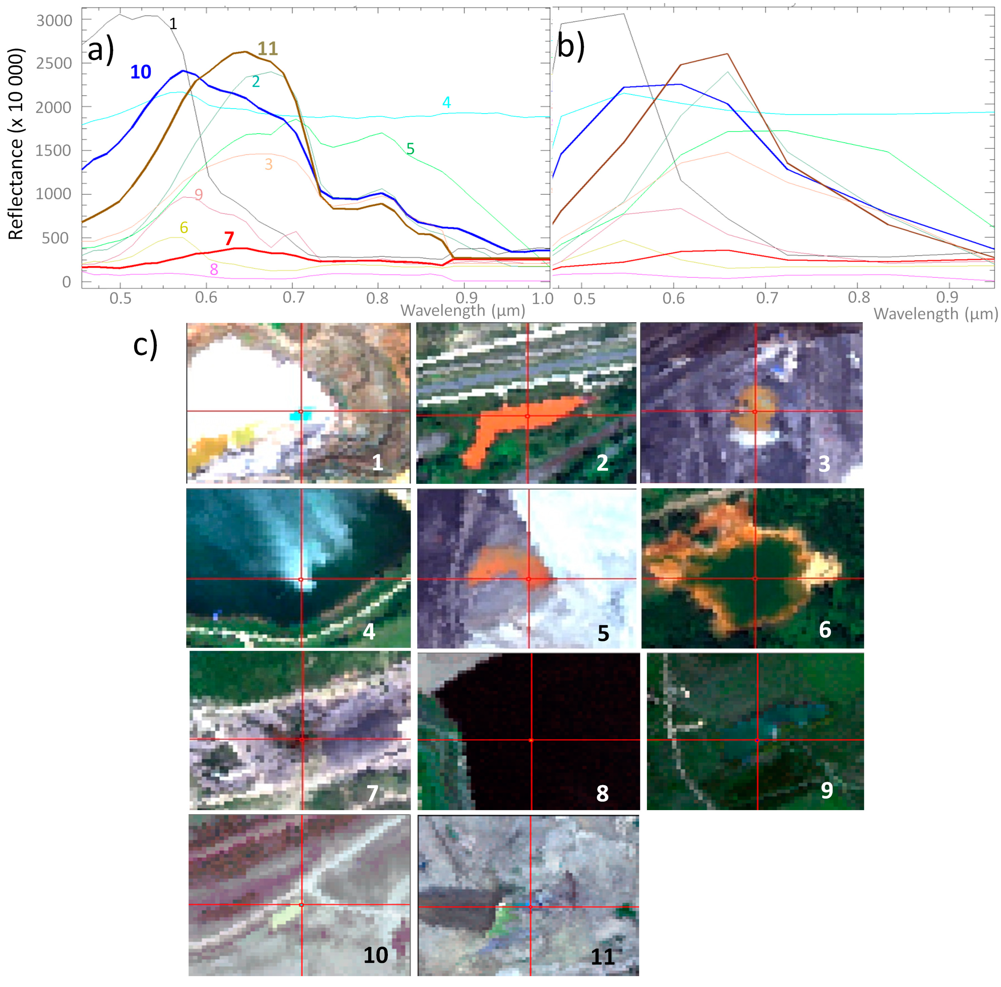
Representative, image-derived end members were extracted for diverse water types: mine waters are rather complex and are characterized by high variability; therefore, the spectral properties of fundamental image end members can provide valuable information on the water constituent types in the study area.

-

Image reflectance data for the derived end members as well as for the sampled waters were compared with the literature to discover whether their spectral and physical-chemical properties correspond and whether the spectral properties can be explained on a physical basis.

-

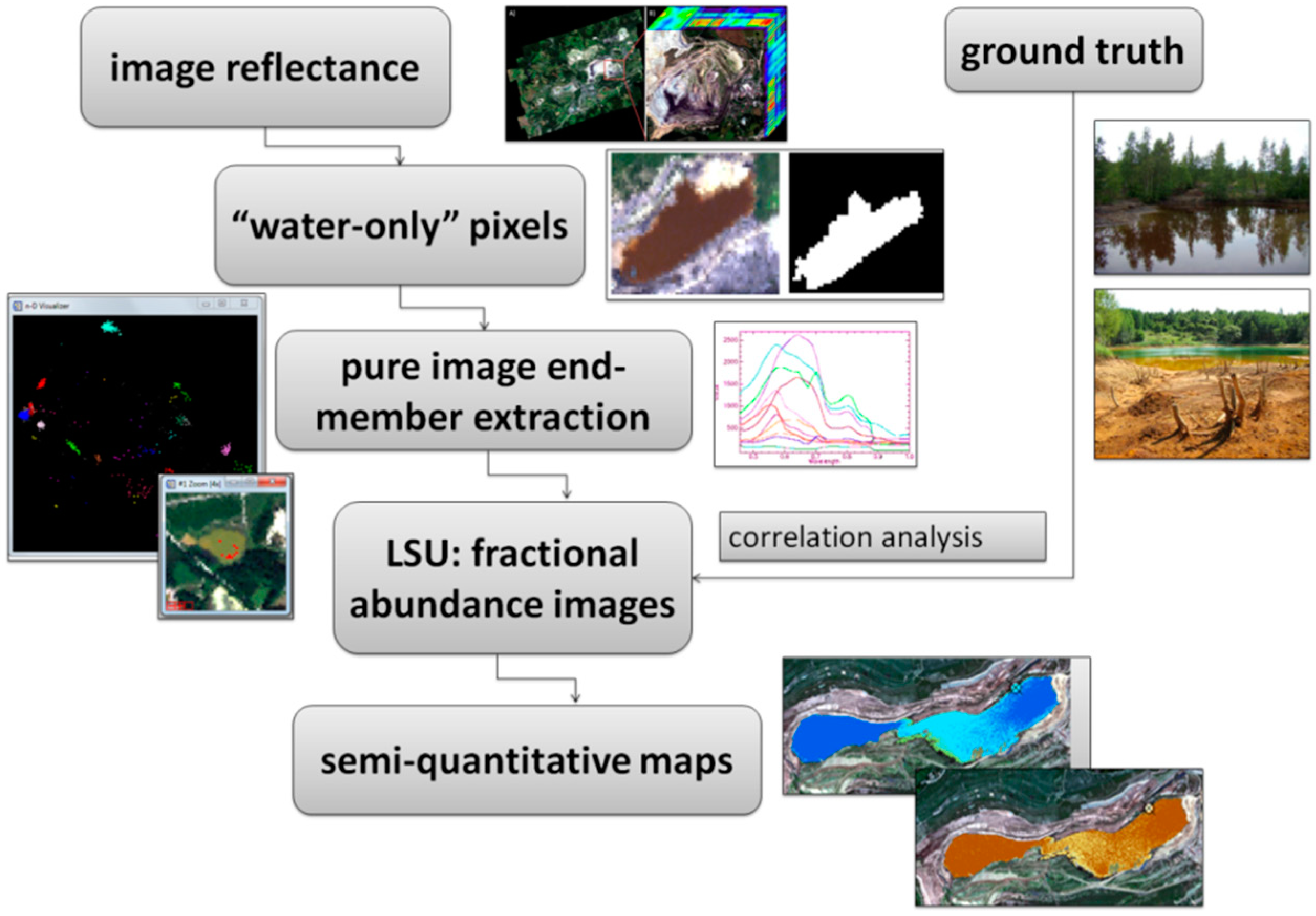
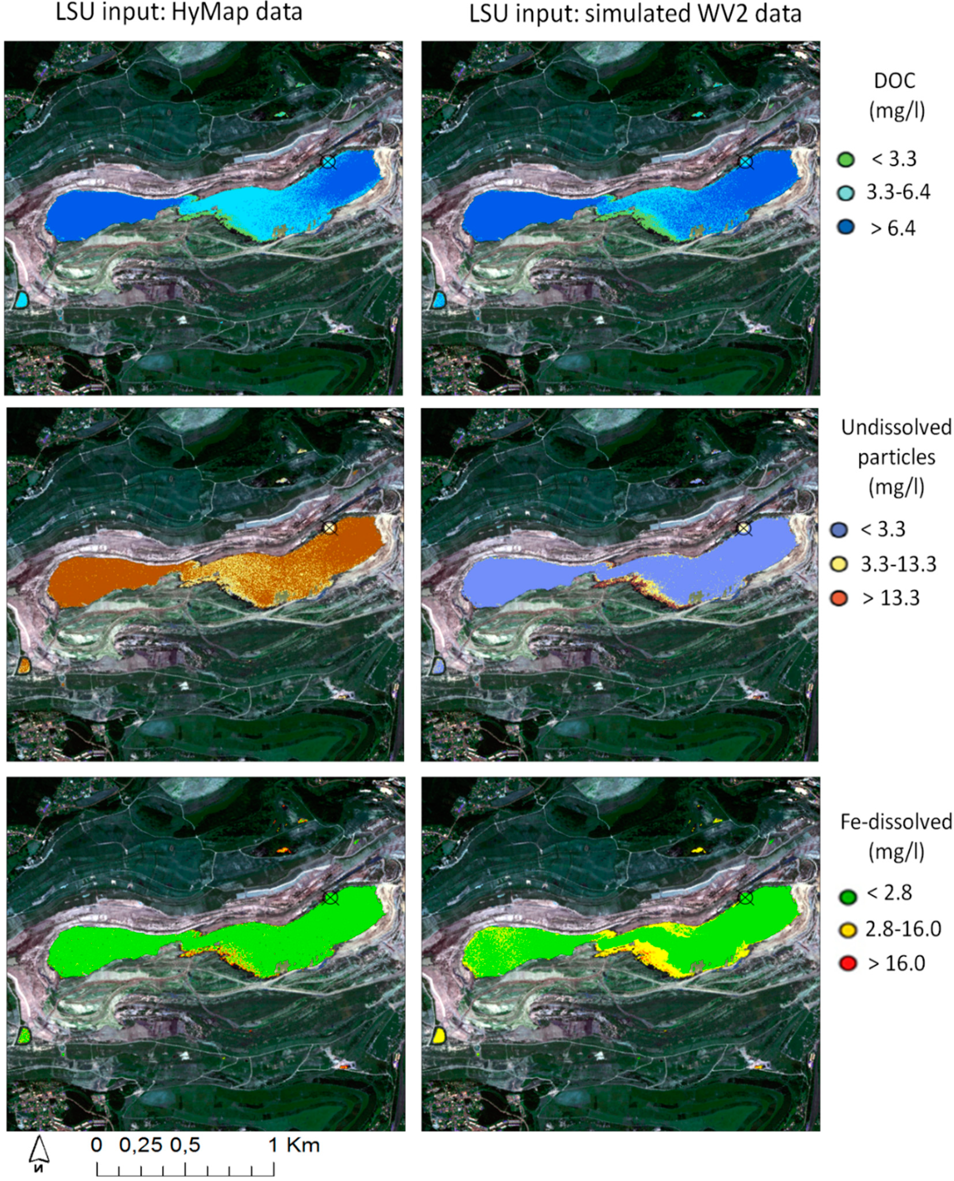
Linear Spectral Unmixing (LSU) was employed and semi-quantitative maps for the selected parameters were created and validated using the ground truth data (hydrochemical data).

-

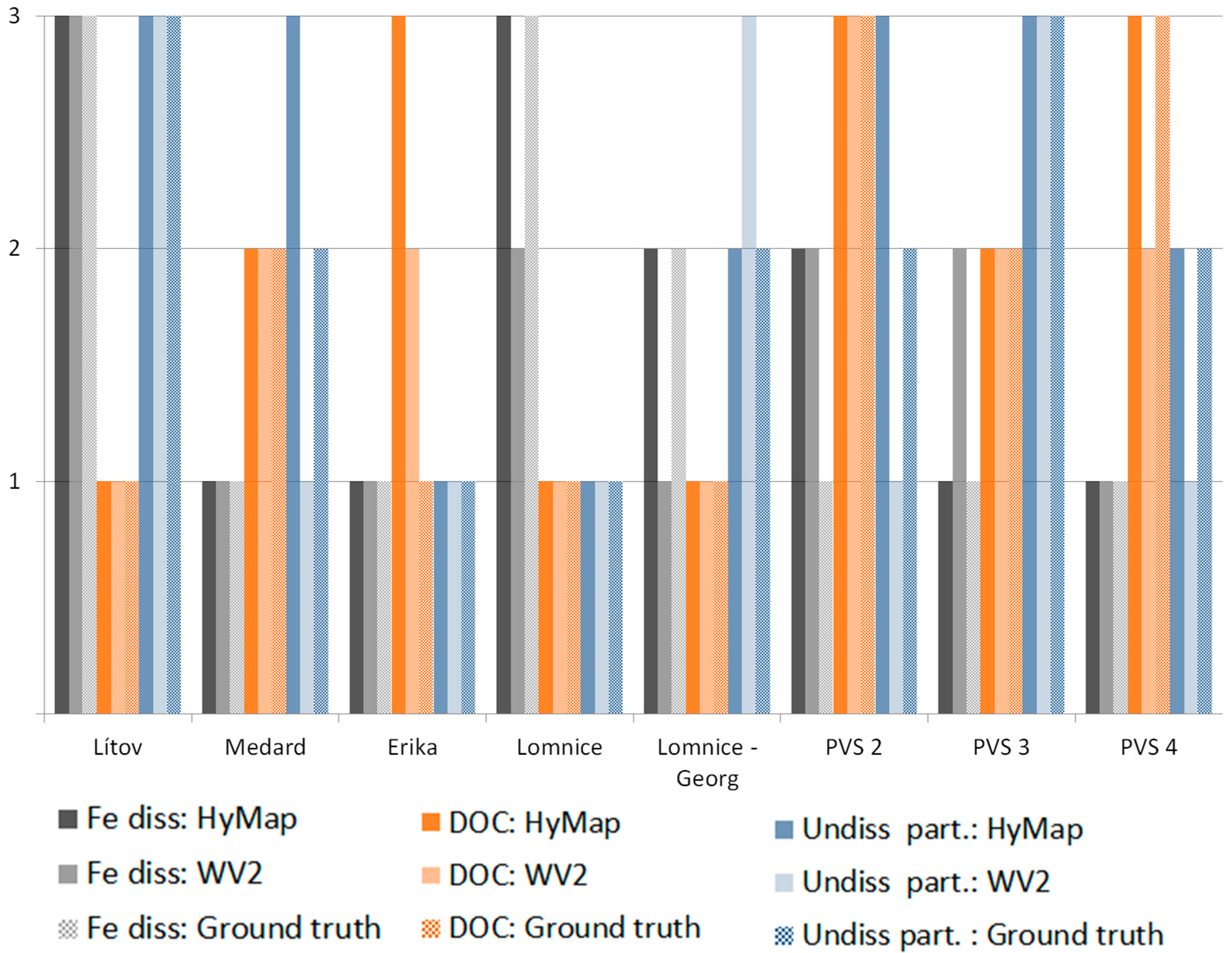
A test was then performed to discover whether the same approach can be employed successfully using the HyMap image data resampled to World View 2 spectra resolution.

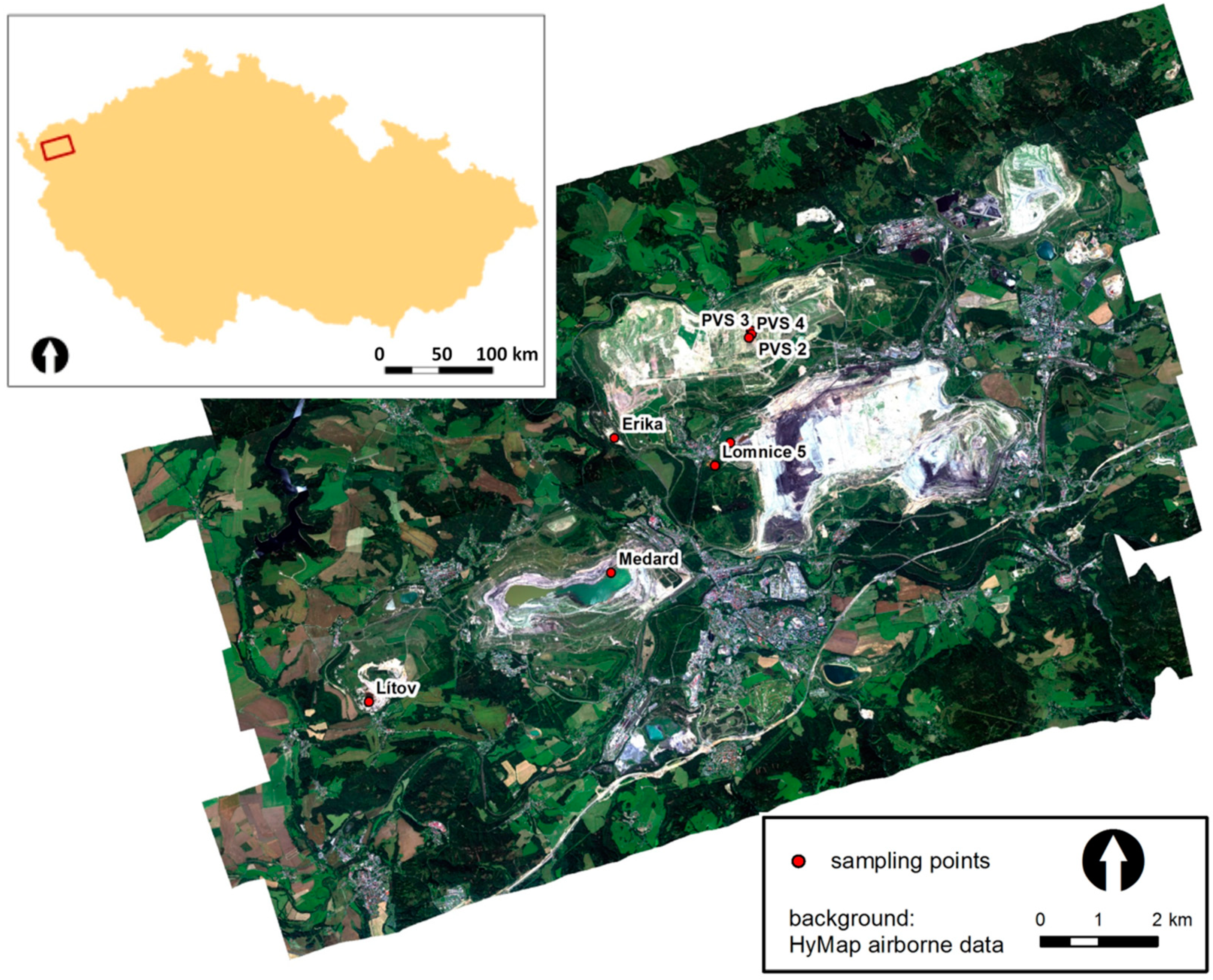
1.1. Test Site

The study was performed in the Sokolov basin in the Western part of the Czech Republic, in a region affected extensive by long-term lignite mining. The basement of the Sokolov Basin is formed of Variscan and pre-Variscan metamorphic complexes of the Eger, Erzgebirge, Slavkov Forest, Thuring-Vogtland Crystalline Units and granitoids of the Karlovy Vary Pluton. The upper portions of these rocks are frequently weathered to a kaolinitic residue. The basal late Eocene Staré-Sedlo-Formation is formed of well-sorted fluvial sandstones and conglomerates and is overlain by an up to 350 m thick volcano-sedimentary complex, which contains three lignite seams with a variable sulfur (S) contents. Material at the dumps, consists mostly of Cypris clays, which can be characterized as well-laminated clays with varying mineralogical compositions: kaolinite, montmorillonite, illite with admixtures of Ca-Mg-Fe carbonates, sulphates, sulphides, analcite, Mg-micas and bitumen [25]. Because of the presence of S in the coal, the mining sites are largely affected by acid mine drainage (AMD) ([26,27,28]).

The mining site is characterized by extreme dynamics, material heterogeneity, high pH gradients and widely varying surface water pollution. In 2009, diverse abandoned pits and dumps could be found within the lignite basin together with still-operating mines as well as many artificial ponds with different chemical and physical properties (Figure 1).

Figure 1. Test site: sampling/measuring points displayed on the HyMap 2009 data (corrected reflectance, true color coding).

Figure 1. Test site: sampling/measuring points displayed on the HyMap 2009 data (corrected reflectance, true color coding).

1.2. Hyperspectral Image Data

The hyperspectral image data (9 flight lines) were acquired in 2009 (July 27) during the HyEUROPE 2009 flight campaign using the HyMap (HyVista Corp., Australia) airborne imaging spectrometer. The HyMap sensor records image data in 126 narrow spectral bands covering the entire spectral interval between 0.450 and 2.480 µm in the spectral range with Full Width Half Maximum (FWHM) of 15 nm and ground field of view of 4 m. The resulting ground pixel resolution of the image datasets was 5 m. The 2009 HyMap multiple flight line data were atmospherically corrected using software (SW) package ATCOR-4 version 5.0 [29]. In addition to the atmospheric correction, the 2009 reflectance data had to be further processed to minimize the Bidirectional Reflectance Distribution Function (BRDF) effect employing semi-empirical nadir normalization with the kernel-based Ross-Li model for all the flight lines (further detailed description on the HyMap 2009 data pre-processing in [30]). Finally, the hyperspectral image data were ortho-rectified using PARGE SW and georeferenced to the UTM 33N (WGS-84) coordinate system.

Once the image preprocessing was complete, a “water-only” image was produced employing a maximum likelihood supervised classification method. As the water SIOPs mainly vary in the visible and near infrared spectral regions (VNIR), only the first 35 HyMap bands covering the VNIR spectrum were selected and subsequent image analysis was applied to the water-only pixels (Section 1.3), characterized by bands covering the 0.45–1.00 µm spectral region. The optical properties were compared with the measured water quality data (Figure 1 and also Section 1.3) by extraction of the image reflectance for the pixels corresponding to the sampling locations.

1.3. Ground Truth Data

One week after the flight campaign, a field trip was organized to investigate the general chemical and physical properties of the Sokolov surface waters. The weather and hydro-meteorological conditions remain unchanged; therefore, the authors assume that the conditions in the studied waters remained similar enough to allow comparison between the ground truth data and the image analysis outputs. Seventeen water sites were selected (Figure 1 and Figure 2) where the pH, Eh, conductivity (Con) and redox potential were determined using a field pH-Eh meter (pH/Cond 340i), together with temperature (T) at the site. Four in-situ measurements were taken at each sampling point to determine the pH, Eh and T. In addition, three samples were taken from the uppermost 30 cm of water to determine the other parameters—dissolved Fe, DOC, undissolved particles—these samples were treated following laboratory standards. All the samples were immediately placed in a cooler and then transferred to a refrigerator, where they were stored until transport to the certified laboratories of the Czech Geological Survey. They were then analyzed using standard methods: (i) dissolved Fe (ČSN EN ISO17025)—the iron (Fe) was analyzed in filtered water samples (0.45 µm filter pore size); the water samples were then acidified using concentrated HNO₃ (0.5 mL/100 mL) and dissolved Fe was determined using the PE-3100AA spectrometer; (ii) DOC (EN 1484:1997): water was filtered using a diafragmal filter (0.45 µm pore size), inorganic carbon was removed by acidification and purging, the CO₂ formed by oxidation was determined after reduction and the final determination of CO₂ was carried out by infrared spectrophotometry; (iii) undissolved particles ČSNEN 872 (757349)—the samples were filtered using a 0.45 mm millipore syringe filter.

Figure 2. Sampled waters: boxplots of the major parameters further discussed in the text. Boxes indicate the variations as defined by the standard deviation; the median is indicated as a horizontal line in the box; Quartile 1 and Quartile 3 indicate the minimum and maximum values, respectively.

Figure 2. Sampled waters: boxplots of the major parameters further discussed in the text. Boxes indicate the variations as defined by the standard deviation; the median is indicated as a horizontal line in the box; Quartile 1 and Quartile 3 indicate the minimum and maximum values, respectively.

Figure 2 shows the basic statistics for the studied water parameters. The water pH varied between 3.0 and 8.5 with a median value of pH 4.2. The dissolved Fe concentrations varied between 0 and 120 mg/L; however, at low pH values (<3.5), the concentration varied between 25 and 120 mg/L which is in agreement with [15]. DOC could be found at a concentration up to 9.0 mg/L; these concentrations are also comparable with the results for mine waters published by [15]. Undissolved particle concentrations ranged between 0.5 and 16.0 mg/L with a median value of 12.0 mg/L.

1.4. Spectral Mapping Methods

The general processing scheme is depicted in Figure 3. Image end members were derived from the “water-only” pixels and used for further image processing. A method consisting of minimum noise fraction transformation (MNF) [31,32] and pixel purity index (PPI) [33] procedures was employed to select the “pure” image end members. In this routine, the image data are subjected to spectral and spatial reduction to identify the end members of spectrally unique pixels, which are assumed to be the most pure. The MNF bands were plotted in scatterplots to examine the distribution of the data in feature space and the nature of the spectral mixing. The spectral end members were identified from the scatterplots of various MNF band combinations, using a similar approach to [8,34,35]. The end members in the feature space were highlighted to identify the pixels represented in the image. It was anticipated that application of this procedure to the hyperspectral image data would yield the spectra of all the fundamental water types differing in their chemical compositions and physical properties.

Figure 3. Processing scheme used for the HyMap image reflectance data as well as for the image reflectance resampled to WV2 spectral resolution.

Figure 3. Processing scheme used for the HyMap image reflectance data as well as for the image reflectance resampled to WV2 spectral resolution.

The image end members were then used to unmix their relative contributions, using ENVI, on a pixel-by-pixel basis to produce images of the relative abundance of each of the identified end members. The linear spectral unmixing (LSU) [36] method was employed to relatively estimate the selected end-member abundances, as it allows identification of the sub-components of the spectrum and determination of the abundances of different materials for each pixel. The linear spectral mixture modeling framework can be expressed mathematically:

$$R_i(\lambda )={\displaystyle \sum _{j=1}^n{F}_j{R}_f{(\lambda )}_i+{\epsilon }_i}$$

(1)

$$0\le {\displaystyle \sum _{j=1}^0{F}_j\le 1}$$

(2)

where R_i is the composite reflectance of the mixed spectrum in band i, F_j the fraction of the end member (j) in the mixture, R_f is the reflectance of that end member in band i, n is the number of end members, ε is the error in sensor band i and λ is the wavelength. Equation (2) constrains the fractions that can have values between 0 and 1. The above equations implicitly assume that each cover type contributes linearly to the pixel reflectance and thus there are negligible non-linear interactions between the end members.

The LSU method has already been employed by [37,38,39,40,41] to model more complex water properties. Spectral mixture analysis is based on the principle that the reflectance recorded for each pixel within an image is a combination of the reflectance from all the pure end members found in that image. The result is an image band for each end member containing the relative abundances of the material within each pixel. These fractional images can be used to constrain additional spectral analyses, as input to biophysical and biogeochemical models [42]. Although the derived end members did not have to be absolutely pure, they represented the most extreme water types found within the studied areas. The authors thus assumed that that linear mixing was a sufficient first-order approximation to constrain the relative abundances.

After the fractional images were derived as the results of LSU, it was desirable to select only those exhibiting a statistical relationship to the studied hydrochemical parameters. Therefore, all the fractional images were compared with the field data collected from the discrete locations (e.g., the ground truth data). The correlations between the ground truth data—water samples from the 8 water bodies that were large enough to be resolved under a 5-m pixel of the HyMap data—and the corresponding pixel values of the fractional images were then determined. As a result, three fractional images exhibiting the strongest correlations with the studied parameters (Fe_diss, DOC, undissolved particles) were selected and further utilized for spatial mapping (Section 2.4).

Figure 4. Image spectra (scaled reflectance) of the selected sampling points that best illustrated the discussed gradients: (a) Samples differing in their undissolved particle content. (b) Samples differing in their Fe_diss content. (c) Samples differing in their DOC content, but whose spectral properties show that they are rather complex and contain DOC together with tripton and a mineral suspension. Diagnostic scattering and absorbance features for particular matter (PM), Fe_diss and DOC are also indicated.

Figure 4. Image spectra (scaled reflectance) of the selected sampling points that best illustrated the discussed gradients: (a) Samples differing in their undissolved particle content. (b) Samples differing in their Fe_diss content. (c) Samples differing in their DOC content, but whose spectral properties show that they are rather complex and contain DOC together with tripton and a mineral suspension. Diagnostic scattering and absorbance features for particular matter (PM), Fe_diss and DOC are also indicated.

To test whether the WV2 data can be successfully utilized for this type of application, the HyMap image data were convolved to the WV2 spectral resolution. The following routine convolving a high-resolution data set to a lower-resolution dataset was employed. Information on the central wavelength together with the Full Width at Half Maxima (FWHM) for each WV2 band were used (a response function library of the WV2 data is available under the ENVI 5.0 version) and a Gaussian model was employed using the FWHM spacing. The HyMap and the convolved WV2 spectra of the selected sampling points and image-derived end members are plotted together in Figure 4 and Figure 5 for comparison. The same approach as that described for the HyMap data processing was then applied to the simulated WV2 data (Figure 3) and the classification results were compared.

Figure 5. Image-derived end members used for the LSU: (a) The end members (EM) of the corresponding fractional images exhibiting strongest correlations with the studied hydrochemical parameters are shown in bold (EM 7: Fe_diss, EM10: DOC and EM11: undissolved particles). (b) The same end members resampled to WV2 spectral resolution. (c) Each end member corresponding geographic position: water with high contents of diverse suspended matter (EM1, 4, 10), water with Fe precipitated on mineral suspended matter (EM2), water with high chlorophyll a concentrations (EM9), clear water (EM8), water with high contents of dissolved Fe (EM7), water with high levels of DOC and solid tripton or other particulate matter (EM3 and 11).

Figure 5. Image-derived end members used for the LSU: (a) The end members (EM) of the corresponding fractional images exhibiting strongest correlations with the studied hydrochemical parameters are shown in bold (EM 7: Fe_diss, EM10: DOC and EM11: undissolved particles). (b) The same end members resampled to WV2 spectral resolution. (c) Each end member corresponding geographic position: water with high contents of diverse suspended matter (EM1, 4, 10), water with Fe precipitated on mineral suspended matter (EM2), water with high chlorophyll a concentrations (EM9), clear water (EM8), water with high contents of dissolved Fe (EM7), water with high levels of DOC and solid tripton or other particulate matter (EM3 and 11).

2. Results and Discussion

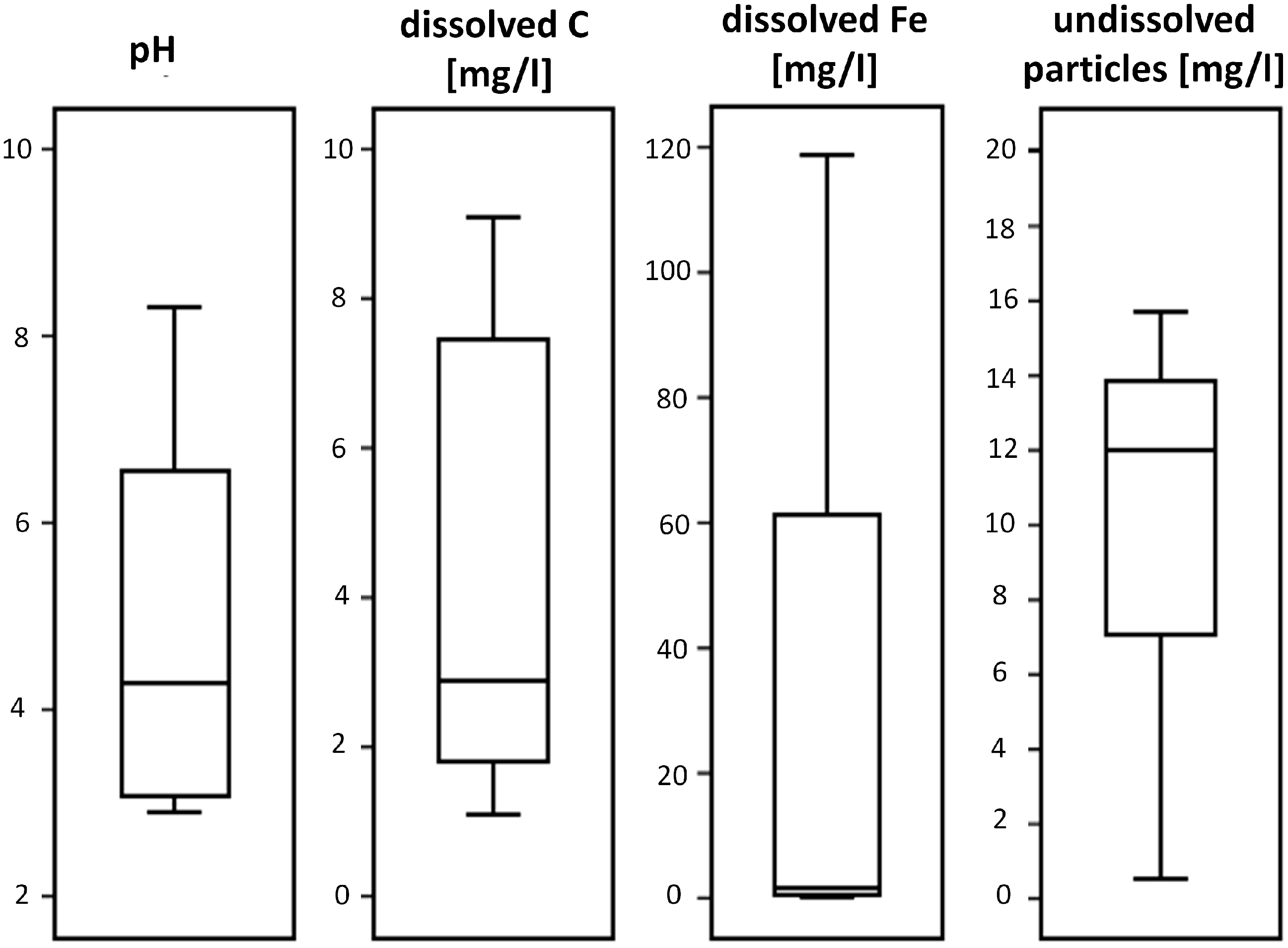
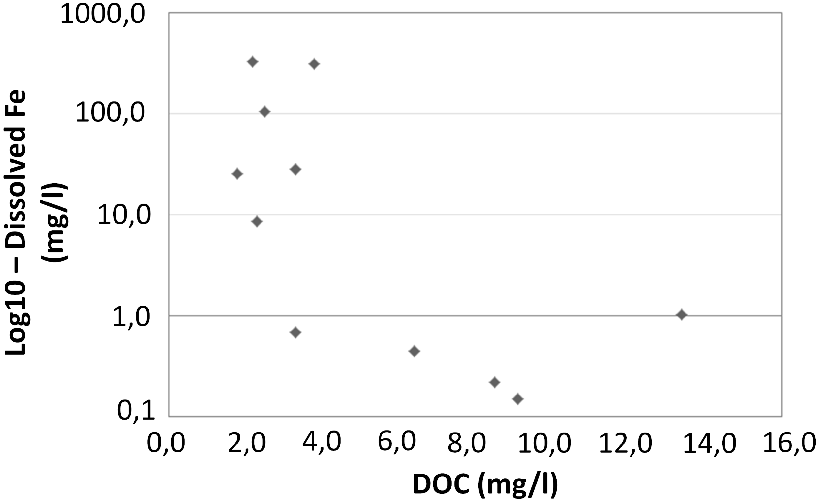
2.1. Linking the Chemical and Optical Properties of the Sampled Waters

To compare chemical and optical properties of the sampled waters, the corresponding pixel image spectra were derived for each sampling point with the following results. Figure 4 shows the image spectra (scaled reflectance) of the selected sampling points that best illustrated the gradients discussed below.

Undissolved particles: Due to scattering from suspended matter, the reflectance increases with the turbidity value in all the parts of the studied spectrum (0.45–1.00 µm, Figure 4a). Waters rich in undissolved particles exhibit the following reflectance peaks—the strongest at 0.55–0.56 µm and additional peaks around 0.70 and 0.81 µm, respectively. This is in agreement with [19,43], as high reflectance in the green (0.56 µm) and red/NIR regions was found for sediment-dominated waters. The region near 0.71 µm was found to correlate positively with the turbidity values [6,16,17,44,45] whereas not being overlapping with the absorptions caused by other optically active substances (e.g., phytoplankton and dissolved organic matter).

Dissolved Fe (Fe_diss): The reflectance at 0.45–0.90 µm was found to be reduced for the samples with high Fe_diss contents, especially in the blue wavelength region, and the location of the peak wavelength moved towards the red region with increasing Fe_diss concentration (Figure 4b). Ritchie, Zimba and Everitt [43] and Glaesser et al. [15] found the same trend, however no other references were found for comparison and discussion of these results.

Dissolved Organic Carbon (DOC): Considering the DOC parameter, it is also important to point out that the relevant optical parameter is not DOC itself, but rather colored dissolved organic matter (CDOM), the photo-active component of DOC. CDOM can be determined from the absorbance of filtered water samples at 420 or 440 nm and conversion of the values to absorptivity values [46]. In 2009 this procedure was not available at the laboratories which performed the water sample analysis. Many studies have reported a correlation greater than 0.9 between CDOM and DOC for marine systems [46,47,48,49]. For freshwaters, good correlation between CDOM and DOC was found by [50,51,52,53,54]; however, on the other hand, some studies reported a weaker relationship [55,56,57]. The authors attempted to link the spectral properties with DOC, although they are aware that DOC is not a direct optical parameter. This aspect is discussed in greater detail in the paper.

A water column with DOC as the only primary component increases the absorption particularly at blue wavelengths and decreases the reflectance across the VIS spectrum, as DOC itself absorbs light across the VIS and produces no significant scattering [44,58,59]. On the other hand, water containing DOC and tripton reflect light primarily in the red and infrared regions. This can be explained by a combination of scattering from tripton and selective absorption by DOC at shorter wavelengths [58]. Image reflectance characterizing waters with high DOC (Figure 4c) contents was obviously represented by optically complex waters. The diagnostic DOC absorption in the blue region was not present; on the other hand, increased reflectance was found throughout the entire studied spectrum (0.45–1.00 µm), pointing to the presence of suspended matter. Similarly as for undissolved particles (Figure 4a), reflectance peaks were found around 0.57 and 0.81 µm; however, the difference between these two peaks is smaller for DOC-rich waters. In addition, the difference between the reflectance at 0.57 and 0.64 µm decreases with increasing DOC content. The typical chlorophyll absorption around 0.69 µm also appears, together with chlorophyll scattering between 0.69 and 0.77 µm [43] (Figure 4c) indicating that the samples contain also tripton. Schalles et al. [60], Schiebe et al. [61] and Ritchie et al. [62] pointed out that the influence of chlorophyll is present even at high suspended sediment concentrations, which can predominate in the remainder of the spectrum. The complex spectral properties discussed above show that the reflectance of the sampled waters, although it corresponds to sufficiently large DOC gradients, is dominating by algal scattering.

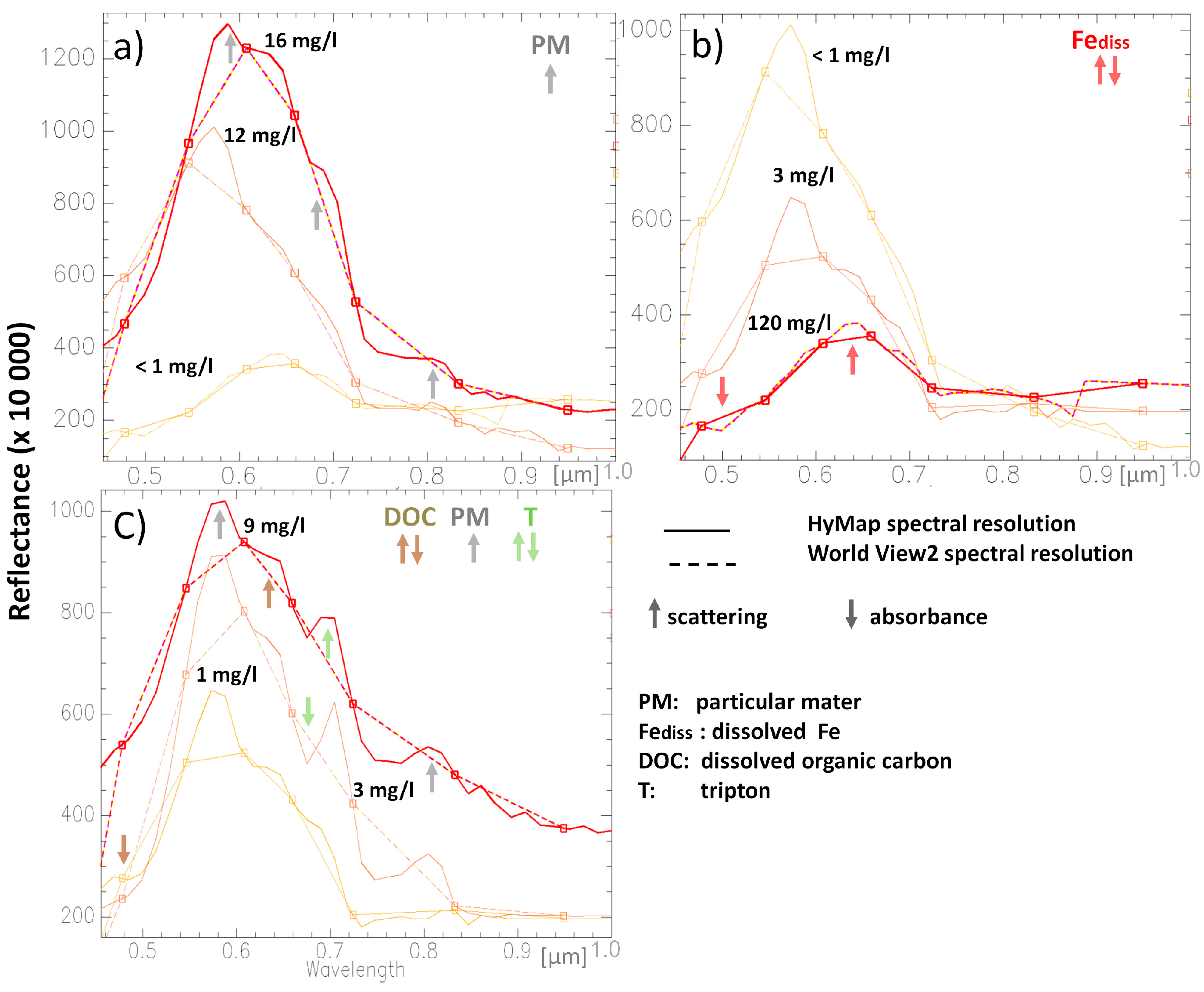
2.2. Reflectance Properties of the Derived Image End Members

Employing the LSU method, 11 “pure” end members were derived for the water-only image pixels (Figure 5a). These end members represented the most extreme water types within the studied area and exhibited large enough differences in spectral shapes as well as in albedo within the studied spectral range (0.45–1.00 µm) (Figure 5). A fraction image was derived for each end member, where each pixel value in this image corresponded to the relative fraction of an end member. The range of fraction values varied between 0 and 1, corresponding to an end member abundance of 0%–100%. All the 11 fractional images derived from LSU were compared with the field data collected from the discrete locations (e.g., the ground truth data). The correlations between the ground truth data and the corresponding pixel values of the fractional images were then determined. Two fractional images, corresponding to end members 7 and 10, exhibited the strongest correlations with the two studied hydrochemical parameters, Fe_diss (R² = 0.72, end member 7: EM7, Table 1) and undissolved particles (R² = 0.57, end member 10: EM10, Table 1), respectively. These two end members (EM7 and EM10, Figure 6a) exhibited basically the same reflectance properties as those already described in 2.1. (“Linking the chemical and optical properties of the sampled waters”, Figure 4a,b). End member 7 exhibited reduced reflectance, especially in the blue wavelength region, and the peak wavelength was located at 0.640 µm. End member 10 exhibited the reflectance peaks typical for sediment-dominated waters, with the strongest at 0.55–0.56 µm and additional peaks around 0.70 and 0.81 µm.

Table 1. Statistics for the linear regression results: water ground truth data and the selected fractional images yielding the highest R².

Variable	End Member n. (Add Figure 5a)	R2 :Hymap/WV2	Sig.: Hymap/WV2
Fe dissolved	EM 7	0.74/0.60	0.006/0.009
DOC	EM 11	0.42/<0.40	0.116/-
Undissolved particles	EM 10	0.57/0.49	0.031/0.044

Table 1. Statistics for the linear regression results: water ground truth data and the selected fractional images yielding the highest R².

Variable	End Member n. (Add Figure 5a)	R2 :Hymap/WV2	Sig.: Hymap/WV2
Fe dissolved	EM 7	0.74/0.60	0.006/0.009
DOC	EM 11	0.42/<0.40	0.116/-
Undissolved particles	EM 10	0.57/0.49	0.031/0.044

The weakest correlation was found between the fractional image and DOC (R² = 0.42, end member 11, Table 1). The reflectance property of the corresponding end member is characterized by typical decreased reflectance in the blue region and a reflectance maximum at the red wavelength (at 0.65 µm) while exhibiting a second reflectance peak at 0.81 µm (EM11, Figure 6). This reflectance can be explained by a combination of scattering from solid tripton or other particulate matter (high red reflectance with a maximum at 0.67 µm, [19,63] and selective absorption by DOC at shorter wavelengths (blue wavelengths: 0.45–0.50 µm). The weak statistical relationship can be explained by a well-known fact that DOC is present in diverse chemical forms (e.g., [64]). In addition, the relevant optical parameter is not DOC itself, but rather colored dissolved organic matter (CDOM). As stated above, many studies reported excellent correlations between CDOM and DOC; however, the relationship between these two parameters may be more complicated because of diverse environmental factors as well as anthropogenic contaminations [56,65]. Not all DOC is colored and therefore the introduced uncertainty in the relationship between DOC and CDOM could also explain the weak correlation [57].

Figure 6. Sampled water characteristics: high contents of dissolved Fe were present when there were low DOC concentrations (<5 mg/L).

Figure 6. Sampled water characteristics: high contents of dissolved Fe were present when there were low DOC concentrations (<5 mg/L).

2.3. Spectral Resolution Issues: Hyperspectral (HyMap) vs. Multispectral (WorldView2)

Although R² describing the linear relationship between the studied water variables and corresponding fractional abundances of unmixed images decreased when the simulated WV2 data was used, the achieved results for Fe_diss and the undissolved particles are still acceptable (Table 1, WV2: Fe_diss: R²_WV2 = 0.60, Undissolved particles: R²_WV2 = 0.49). In contrast, a statistically significant linear relationship was not obtained for DOC (Table 1, R²_WV2 < 0.40). In the comparison of the hyperspectral (HyMap) and multispectral (WV2) properties of the sampled waters (Figure 4a–c) and the image end members (Figure 5a), the shapes or general trends are preserved, but the subtle details obtained using HS data, especially at 0.45–0.50, 0.65–0.70 and 0.72–0.90 µm, are missing. These differences can mean that the weak relationship which was still detectable under the HyMap spectral resolution was no longer detected using the WV2 resampled data. The differences between the end members representing Fe_diss and the undissolved particles are still large enough, but those between the end members of the undissolved particles and DOC are no longer sufficient.

2.4. Semi-Quantitative Maps

Before assessing the classification results of LSU images, it is necessary to mention that mine waters represent an extreme water type that is heavily polluted. The water column for these extreme waters is not transparent (Figure 5c) and the substrate (e.g., submerged macrophytes and sandy bottoms in lakes) signal cannot be detected through the water column in most cases. Therefore, the depth and the bottom albedo aspect [1] have not been taken into account in this particular case.

Figure 7. Lomnice-Georg: Semi-quantitative maps derived for dissolved organic carbon (DOC), undissolved particles and dissolved Fe. The legend is uniform for both the classified map and for the sampling point.

Figure 7. Lomnice-Georg: Semi-quantitative maps derived for dissolved organic carbon (DOC), undissolved particles and dissolved Fe. The legend is uniform for both the classified map and for the sampling point.

The results of the classifications of the EnMap and the WV2 convolved image data are displayed in Figure 7, Figure 8 and Figure 9. The HyMap LSU fractional images were classified and enabled differentiation among low, middle and high contents for all three studied parameters—DOC, undissolved particles and Fe_diss. Surprisingly, even DOC was classified satisfactorily in these basic classes, although it exhibited the weakest relationship (R² = 0.42). Furthermore, the classifications show that a reciprocal relationship exists between the contents of dissolved C and dissolved Fe. In other words, waters rich in dissolved Fe were depleted in dissolved C and vice versa. The same chemical pattern was found in the hydrochemical properties of the sampled waters (Figure 6). This is not a common trend that can be found in natural waters with more representative concentrations of dissolved Fe. Instead, positive correlations between DOC and dissolved Fe are common at higher pH values (>5), where the dissolved Fe is primarily associated with dissolved organic ligands such as HS or siderophores [66,67,68]. The trend described in this paper could be related to the pH, as the waters with very high Fe_diss had low pH, and DOC levels could have been depressed because of the tendency of iron to coagulate and precipitate DOC at low pH values [64].

Figure 8. Medard: Semi-quantitative maps derived for dissolved organic carbon (DOC), undissolved particles and dissolved Fe. The legend is uniform for both the classified map and for the sampling point.

Figure 8. Medard: Semi-quantitative maps derived for dissolved organic carbon (DOC), undissolved particles and dissolved Fe. The legend is uniform for both the classified map and for the sampling point.

Figure 9. Validation of semi-quantitative mapping: the corresponding pixel values of the classified maps (classified LSU fractional images) are compared to the classified values of the ground truth data. Classes 1, 2 and 3 (Y axis) correspond to low, middle and high content classes for DOC, undissolved particles and Fe_diss displayed in Figure 7 and Figure 8.

Figure 9. Validation of semi-quantitative mapping: the corresponding pixel values of the classified maps (classified LSU fractional images) are compared to the classified values of the ground truth data. Classes 1, 2 and 3 (Y axis) correspond to low, middle and high content classes for DOC, undissolved particles and Fe_diss displayed in Figure 7 and Figure 8.

Waters rich in DOC were found mainly in former lignite mines (e.g., Medard, Lomnice-Georg, Podkrušnohorská-PVS, Figure 7, Figure 8 and Figure 9), where the lignite seam is exposed and thus accessible for weathering. Waters rich in Fe_diss can be found in environments characterized by very low pH, such as Lítov (Figure 9), the site characterized by the lowest pH among the Sokolov mines and dumpsites [27,28].

Comparison of the HyMap and WV2 classifications showed good agreement, especially for Fe_diss. Basically, the same patterns were identified (Figure 7, Figure 8 and Figure 9) using either the HyMap or convolved WV2 image data as inputs of LSU. For the undissolved particles, good agreement was found for some sites (e.g., Litov, Lomnice and Erika, Figure 9). On the other hand, the WV2 classification for Medard (Figure 8) and Podkrušnohorská-PVS2 (Figure 9) exhibited low values while the HyMap classification yielded the opposite results—high values. This misclassification can be explained by the high spectral similarity of the WV2 resampled spectra of the end members for DOC and undissolved particles. The high spectral similarity increases a level of collinearity in the end-member matrix, which makes the unmixing model more unstable and more sensitive to random error (e.g., noise) [69].

3. Conclusions

This paper demonstrates that the LSU method can be utilized to map selected water parameters at a semi-quantitative level using HyMap or World View2 image data even when there is a limited amount of ground truth data. LSU was tested on polluted mine waters which differ significantly from natural waters. A key aspect was to define the proper pure image end members for the fundamental water types (water rich in suspended solids and dissolved Fe and DOC). Although the derived end members did not have to be absolutely pure, they represented the most extreme water types within the studied area and exhibited large enough differences in spectral shapes as well as in albedo within the studied spectral range (0.45–1.00 µm). However, the demonstrated method can also be successfully employed for other waters as long as the water end-members are sufficiently spectrally different (uncorrelated) and don’t cause end-member matrix (multi-)collinearity [69].

Correlations between the studied water parameters and the three fractional images were detected for the HyMap data and the resampled WV2 data, respectively: dissolved Fe (R² = 0.74 and R²_vw2 = 0.6), undissolved particles (R² = 0.57 and R²_vw2 = 0.49) and DOC (R² = 0.42 and R²_vw2 < 0.40). Either utilizing the HyMap or the convolved WV2 image data, the selected LSU fractional images enabled differentiation among low, middle and high contents for all three studied parameters—DOC, undissolved particles and Fe_diss.

In conclusion, the classifications still benefited from the higher spectral resolution of the HyMap data; however, the WV2 reflectance data can be sufficient for mapping SIOPs, which significantly differ from an optical point of view (e.g., mineral suspension and dissolved Fe) but cannot really differentiate among diverse suspended particles (e.g., mineral particles, DOC together with tripton or adsorbed on other particles, etc.). On the other hand, mapping and classification of mine waters, which usually have rather small spatial extent, may still benefit from the higher spatial resolution of the WV2 data. In this paper, only the WV2 spectral resolution was simulated; however the spatial resolution was limited to 5 m—the original spatial resolution of the HyMap data.

The study also demonstrates that these methods could be used to classify mine waters into basic groups. As water sampling is very time-consuming and costly, this can improve the efficiency of water sampling/monitoring or be used to support further detailed investigations leading to quantitative spectral mapping. Processing time can be saved when temporal changes are studied by deriving the end members from an image acquired under the most extreme weather conditions, when the concentrations of the studied components are the highest. These end members can be then utilized for spectral mapping of other temporal image data.

Only a limited number of papers have been published to date on mine water pollution and how image spectroscopy could be used for this aspect. Therefore, more systematic work to link optical and physical-chemical properties of waters should be performed in the future.

References and Notes

1. Roessler, S.; Wolf, P.; Schneider, T.; Zimmermann, S.; Melzer, A. Water constituent retrieval and littoral bottom mapping using hyperspectral apex imagery and submersed artificial surfaces. EARSeL eProc. 2013, 1, 44–57. [Google Scholar]
2. Stroembeck, N. Water quality and optical properties of Swedish lakes and coastal waters in relation to remote sensing. In Comprehensive Summaries of Uppsala Dissertations from the Faculty of Science and Technology; Karlstads University: Karlstad, Sweden, 2001; Volume 633, p. 27. [Google Scholar]
3. Ambarwulan, W.; Salama, M.S.; Mannaerts, C.M.; Verhoef, W. Estimating specific inherent optical properties of tropical coastal waters using bio-optical model inversion and in situ measurements: Case of the Berau estuary, East Kalimantan, Indonesia. Hydrobiologia 2011, 658, 197–211. [Google Scholar] [CrossRef]
4. Koponen, S.; Pulliainen, J.; Kallio, K.; Vepsalainen, J.; Hallikainen, M. Use of MODIS data for monitoring turbidity in Finnish lakes. In Proceedings of the 2001 IEEE International Geoscience and Remote Sensing Symposium, Sydney, Australia, 9–13 July 2001; pp. 2184–2186.
5. Koponen, S.; Pulliainen, J.; Servomaa, H.; Zhang, Y.; Hallikainen, M.; Kallio, K.; Vepsalainen, J.; Pyhalahti, T.; Hannonen, T. Analysis on the feasibility of multi-source remote sensing observations for chl-a monitoring in Finnish lakes. Sci. Total Environ. 2001, 268, 95–106. [Google Scholar] [CrossRef] [PubMed]
6. Koponen, S.; Attila, J.; Pulliainen, J.; Kallio, K.; Pyhalahti, T.; Lindfors, A.; Rasmus, K.; Hallikainen, M. A case study of airborne and satellite remote sensing of a spring bloom event in the Gulf of Finland. Cont. Shelf Res. 2007, 27, 228–244. [Google Scholar] [CrossRef]
7. Pulliainen, J.; Kallio, K.; Eloheimo, K.; Koponen, S.; Servomaa, H.; Hannonen, T.; Tauriainen, S.; Hallikainen, M. A semi-operative approach to lake water quality retrieval from remote sensing data. Sci. Total Environ. 2001, 268, 79–93. [Google Scholar] [CrossRef] [PubMed]
8. Thiemann, S.; Kaufmann, H. Lake water quality monitoring using hyperspectral airborne data—A semiempirical multisensor and multitemporal approach for the Mecklenburg Lake District, Germany. Remote Sens. Environ. 2002, 81, 228–237. [Google Scholar] [CrossRef]
9. Doxaran, D.; Castaing, P.; Lavender, S.J. Monitoring the maximum turbidity zone and detecting fine-scale turbidity features in the Gironde estuary using high spatial resolution satellite sensor (SPOT HRV, Landsat ETM+) data. Int. J. Remote Sens. 2006, 27, 2303–2321. [Google Scholar] [CrossRef]
10. Harrington, J.A.; Schiebe, F.R.; Nix, J.F. Remote sensing of Lake Chicot, Arkansas: Monitoring suspended sediments, turbidity, and Secchi depth with Landsat MSS Data. Remote Sens. Environ. 1992, 39, 1–27. [Google Scholar] [CrossRef]
11. Santini, F.; Alberotanza, L.; Cavalli, R.M.; Pignatti, S. A two-step optimization procedure for assessing water constituent concentrations by hyperspectral remote sensing techniques: An application to the highly turbid Venice lagoon waters. Remote Sens. Environ. 2010, 114, 887–898. [Google Scholar] [CrossRef]
12. Huang, C.; Chen, X.; Li, Y.; Yang, H.; Sun, D.; Li, J.; Le, C.; Zhou, L.; Zhang, M.; Xu, L. Specific inherent optical properties of highly turbid productive water for retrieval of water quality after optical classification. Environ. Earth Sci. 2014. [Google Scholar] [CrossRef]
13. Matthews, M.W.; Bernard, S. Characterizing the absorption properties for remote sensing of three small optically-diverse South African reservoirs. Remote Sens. 2013, 5, 4370–4404. [Google Scholar] [CrossRef]
14. Frauendorf, J. Entwicklung und Anwendung von Fernerkundungsmethoden zur Ableitung von Wasserqualitätsparametern Verschiedener Restseen des Braunkohlentagebaus in Mitteldeutschland. PhD Thesis, Martin Luther University Halle Wittenberg, Halle, Germany, 2002. [Google Scholar]
15. Glaesser, C.; Groth, D.; Frauendorf, J. Monitoring of hydrochemical parameters of lignite mining lakes in Central Germany using airborne hyperspectral casi-scanner data. Int. J. Coal Geol. 2011, 86, 40–53. [Google Scholar] [CrossRef]
16. Harma, P.; Vepsalainen, J.; Hannonen, T.; Pyhalahti, T.; Kamari, J.; Kallio, K.; Eloheimo, K.; Koponen, S. Detection of water quality using simulated satellite data and semi-empirical algorithms in Finland. Sci. Total Environ. 2001, 268, 107–121. [Google Scholar] [CrossRef] [PubMed]
17. Kallio, K.; Kutser, T.; Hannonen, T.; Koponen, S.; Pulliainen, J.; Vepsalainen, J.; Pyhalahti, T. Retrieval of water quality from airborne imaging spectrometry of various lake types in different seasons. Sci. Total Environ. 2001, 268, 59–77. [Google Scholar] [CrossRef] [PubMed]
18. Lee, Z.P.; Carder, K.L.; Steward, R.G.; Peacock, T.G.; Davis, C.O.; Patch, J.S. An empirical algorithm for light absorption by ocean water based on color. J. Geophys. Res. 1998, 103, 27967–27978. [Google Scholar] [CrossRef]
19. Olmanson, L.G.; Brezonik, P.L.; Bauer, M.E. Airborne hyperspectral remote sensing to assess spatial distribution of water quality characteristics in large rivers: The Mississippi River and its tributaries in Minnesota. Remote Sens. Environ. 2013, 130, 254–265. [Google Scholar] [CrossRef]
20. Albert, A.; Mobley, C.D. An analytical model for subsurface irradiance and remote sensing reflectance in deep and shallow case-2 waters. Opt. Express 2003, 11, 2873–2890. [Google Scholar] [CrossRef] [PubMed]
21. Doxaran, D.; Cherukuru, N.; Lavender, S.J. Apparent and inherent optical properties of turbid estuarine waters: Measurements, empirical quantification relationships, and modeling. Appl. Opt. 2006, 45, 2310–2324. [Google Scholar] [CrossRef] [PubMed]
22. Lee, Z.P.; Carder, K.L.; Mobley, C.D.; Steward, R.G.; Patch, J.S. Hyperspectral remote sensing for shallow waters. I. A semianalytical model. Appl. Opt. 1998, 37, 6329–6338. [Google Scholar] [CrossRef] [PubMed]
23. Gege, P. The water color simulator WASI: An integrating software tool for analysis and simulation of optical in situ spectra. Comput. Geosci. 2004, 30, 523–532. [Google Scholar] [CrossRef]
24. DigitalGlobe. The Benefits of the 8 Spectral Bands of Worldview-2. Available online: http://worldview2.digitalglobe.com/docs/WorldView-2_8-Band_Applications_Whitepaper.pdf (accessed on 1 March 2009).
25. Rojík, P. New stratigraphic subdivision of the tertiary in the Sokolov Basin in Northwestern Bohemia. J. Czech Geol. Soc. 2004, 49, 173–186. [Google Scholar]
26. Kopackova, V.; Chevrel, S.; Bourguignon, A.; Rojik, P. Application of high altitude and ground-based spectroradiometry to mapping hazardous low-pH material derived from the Sokolov open-pit mine. J. Maps 2012, 8, 220–230. [Google Scholar] [CrossRef]
27. Kopackova, V. Using multiple spectral feature analysis for quantitative pH mapping in a mining environment. Int. J. Appl. Earth Obs. Geoinf. 2014, 28, 28–42. [Google Scholar] [CrossRef]
28. Lhotakova, Z.; Brodsky, L.; Kupkova, L.; Kopackova, V.; Potuckova, M.; Misurec, J.; Klement, A.; Kovarova, M.; Albrechtova, J. Detection of multiple stresses in Scots pine growing at post-mining sites using visible to near-infrared spectroscopy. Environ. Sci. Process Impacts 2013, 15, 2004–2015. [Google Scholar] [CrossRef] [PubMed]
29. Guanter, L.; Richter, R.; Kaufmann, H. On the application of the MODTRAN4 atmospheric radiative transfer code to optical remote sensing. Int. J. Remote Sens. 2009, 30, 1407–1424. [Google Scholar] [CrossRef]
30. Kopackova, V.; Misurec, J.; Lhotakova, Z.; Oulehle, F.; Albrechtova, J. Using multi-date high spectral resolution data to assess the physiological status of macroscopically undamaged foliage on a regional scale. Int. J. Appl. Earth Obs. Geoinf. 2014, 27, 169–186. [Google Scholar] [CrossRef]
31. Boardman, J.W.; Kruse, F.A. Automated spectral analysis: A geological example using AVIRIS data, North Grapevine Mountains, Nevada. In Proceedings of the 1994 Thematic Conference on Geologic Remote Sensing—Exploration, Environment, and Engineering, San Antonio, TX, USA, 9–19 May 1994; pp. 407–418.
32. Green, A.A.; Berman, M.; Switzer, P.; Craig, M.D. A transformation for ordering multispectral data in terms of image quality with implications for noise removal. IEEE Trans. Geosci. Remote Sens. 1988, 26, 65–74. [Google Scholar] [CrossRef]
33. Boardman, J.W. Analysis, understanding and visualization of hyperspectral data as convex sets in n-space. Proc. SPIE 1995, 2480, 14–22. [Google Scholar]
34. Adams, J.B.; Smith, M.O.; Gillespie, A.R. Imaging spectroscopy: Interpretation based on spectral mixture analysis. In Remote Geochemical Analysis: Elemental and Mineralogical Composition; Pieters, C.M., Englert, P., Eds.; Cambridge University Press: New York, NY, USA, 1993; pp. 145–166. [Google Scholar]
35. Rainey, M.; Tyler, A.N.; Gilvear, D.J.; Bryant, R.; McDonald, P. Mapping estuarine intertidal sediment size fractions through airborne remote sensing. Remote Sens. Environ. 2003, 86, 480–490. [Google Scholar] [CrossRef]
36. Settle, J.J.; Drake, N.A. Linear mixing and the estimation of ground cover proportions. Int. J. Remote Sens. 1993, 14, 1159–1177. [Google Scholar] [CrossRef]
37. Tyler, A.N.; Svab, E.; Preston, T.; Presing, M.; Kovacs, W.A. Remote sensing of the water quality of shallow lakes: A mixture modelling approach to quantifying phytoplankton in water characterized by high-suspended sediment. Int. J. Remote Sens. 2006, 27, 1521–1537. [Google Scholar] [CrossRef]
38. Jiao, Y.; Wang, S.; Zhou, Y.; Yan, F.; Zhou, W.; Zhu, L. Using unmixing method to retrieve the concentration of Chl-a in Lake Tai. In Proceedings of the 2006 IEEE International Geoscience and Remote Sensing Symposium, Denver, CO, USA, 31 July–4 August 2006; pp. 3427–3429.
39. Stein, D.; Stewart, S.; Gilbert, G.; Schoonmaker, J. Band selection for viewing underwater objects using hyperspectral sensors. Proc. SPIE 1999. [Google Scholar] [CrossRef]
40. Thiemann, S.; Berger, M.; Kaufmann, H. Feasibility study for lake water quality assessment using MIDORI AVNIR data. In Proceedings of the 1998 International Geoscience and Remote Sensing Symposium, Seattle, WA, USA, 6–10 July 1998; pp. 936–938.
41. Alcantara, E.; Barbosa, C.; Stech, J.; Novo, E.; Shimabukuro, Y. Improving the spectral unmixing algorithm to map water turbidity distributions. Environ. Model. Softw. 2009, 24, 1051–1061. [Google Scholar] [CrossRef]
42. Asner, P.; Lobell, B. A biogeophysical approach for automated SWIR unmixing of soils and vegetation. Remote Sens. Environ. 2000, 74, 99–112. [Google Scholar] [CrossRef]
43. Ritchie, J.C.; Zimba, P.V.; Everitt, J.H. Remote sensing techniques to assess water quality. Photogramm. Eng. Remote Sens. 2003, 69, 695–704. [Google Scholar] [CrossRef]
44. Dekker, A.G.; Peters, S.W.M. The use of the Thematic Mapper for the analysis of eutrophic Lakes: A case-study in The Netherlands. Int. J. Remote Sens. 1993, 14, 799–821. [Google Scholar] [CrossRef]
45. Koponen, S.; Pulliainen, J.; Kallio, K.; Hallikainen, M. Lake water quality classification with airborne hyperspectral spectrometer and simulated MERIS data. Remote Sens. Environ. 2002, 79, 51–59. [Google Scholar] [CrossRef]
46. Matsuoka, A.; Bricaud, A.; Benner, R.; Para, J.; Sempere, R.; Prieur, L.; Belanger, S.; Babin, M. Tracing the transport of colored dissolved organic matter in water masses of the Southern Beaufort Sea: Relationship with hydrographic characteristics. Biogeosciences 2012, 9, 925–940. [Google Scholar] [CrossRef]
47. Fichot, C.G.; Benner, R. A novel method to estimate DOC concentrations from CDOM absorption coefficients in coastal waters. Geophys. Res. Lett. 2011, 38, L03610. [Google Scholar]
48. Mannino, A.; Russ, M.E.; Hooker, S.B. Algorithm development and validation for satellite-derived distributions of DOC and CDOM in the U.S. Middle Atlantic Bight. J. Geophys. Res. 2008, 113, C07051. [Google Scholar]
49. Tehrani, N.C.; D’Sa, E.J.; Osburn, C.L.; Bianchi, T.S.; Schaeffer, B.A. Chromophoric dissolved organic matter and dissolved organic carbon from sea-viewing wide field-of-view sensor (SeaWiFS), Moderate Resolution Imaging Spectroradiometer (MODIS) and MERIS Sensors: Case study for the Northern Gulf of Mexico. Remote Sens. 2013, 5, 1439–1464. [Google Scholar] [CrossRef]
50. Zhu, W.; Yu, Q.; Tian, Y.Q.; Becker, B.L.; Zheng, T.; Carrick, H.J. An assessment of remote sensing algorithms for colored dissolved organic matter in complex freshwater environments. Remote Sens. Environ. 2014, 140, 766–778. [Google Scholar] [CrossRef]
51. Kallio, K. Absorption properties of dissolved organic matter in Finnish lakes. Proc. Estonian Acad. Sci. Biol. Ecol. 1999, 48, 75–83. [Google Scholar]
52. Tranvik, L.J. Bacterioplankton growth on fractions of dissolved organic carbon of different molecular weights from humic and clear waters. Appl. Environ. Microbiol. 1990, 56, 1672–1677. [Google Scholar] [PubMed]
53. Zhang, Y.; Qin, B.; Zhu, G.; Zhang, L.; Yang, L. Chromophoric dissolved organic matter (CDOM) absorption characteristics in relation to fluorescence in Lake Taihu, China, a large shallow subtropical lake. Hydrobiologia 2007, 581, 43–52. [Google Scholar] [CrossRef]
54. Spencer, R.G.M.; Hernes, P.J.; Ruf, R.; Baker, A.; Dyda, R.Y.; Stubbins, A.; Six, J. Temporal controls on dissolved organic matter and lignin biogeochemistry in a pristine tropical river, Democratic Republic of Congo. J. Geophys. Res. 2010, 115, G03013. [Google Scholar]
55. Bracchini, L.; Dattilo, A.M.; Hull, V.; Loiselle, S.A.; Martini, S.; Rossi, C.; Santinelli, C.; Seritti, A. The bio-optical properties of CDOM as descriptor of lake stratification. J. Photochem. Photobiol. B 2006, 85, 145–149. [Google Scholar] [CrossRef] [PubMed]
56. Spencer, R.G.M.; Butler, K.D.; Aiken, G.R. Dissolved organic carbon and chromophoric dissolved organic matter properties of rivers in the USA. J. Geophys. Res. 2012, 117, G03001. [Google Scholar]
57. Brezonik, P.L.; Olmanson, L.G.; Finlay, J.C.; Bauer, M.E. Factors affecting the measurement of CDOM by remote sensing of optically complex inland waters. Remote Sens. Environ. 2014, in press. [Google Scholar]
58. Arenz, R.F.; Lewis, W.M.; Saunders, J.F. Determination of chlorophyll and dissolved organic carbon from reflectance data for Colorado reservoirs. Int. J. Remote Sens. 1996, 17, 1547–1566. [Google Scholar] [CrossRef]
59. Witte, W.G.; Whitlock, C.H.; Harriss, R.C.; Usry, J.W.; Poole, L.R.; Houghton, W.M.; Morris, W.D.; Gurganus, E.A. Influence of dissolved organic materials on turbid water optical properties and remote-sensing reflectance. J. Geophys. Res. 1982, 87, 441–446. [Google Scholar] [CrossRef]
60. Schalles, J.; Schiebe, F.; Starksand, P.; Troeger, W. Estimation of algal and suspended sediment loads (singly and combined) using hyperspectral sensors and integrated mesocosm experiments. In Proceedings of the 1997 International Conference on Remote Sensing for Marine and Coastal Environments, Orlando, FL, USA, 17–19 March 1997; pp. 111–120.
61. Schiebe, F.R.; Harrington, J.A.; Ritchie, J.C. Remote sensing of suspended sediments: The Lake Chicot, Arkansas project. Int. J. Remote Sens. 1992, 13, 1487–1509. [Google Scholar] [CrossRef]
62. Ritchie, J.C.; Schiebe, F.R.; Cooper, C.M.; Harrington, J.A. Landsat-MSS studies of chlorophyll in sediment dominated lakes. In Proceedings of the 1992 International Geoscience and Remote Sensing Symposium, Houston, TX, USA, 26–29 May 1992; pp. 1514–1517.
63. Hirtle, H.; Rencz, A. The relation between spectral reflectance and dissolved organic carbon in lake water: Kejimkujik National Park, Nova Scotia, Canada. Int. J. Remote Sens. 2003, 24, 953–967. [Google Scholar] [CrossRef]
64. Koehler, S.J.; Kothawala, D.; Futter, M.N.; Liungman, O.; Tranvik, L. In-lake processes offset increased terrestrial inputs of dissolved organic carbon and color to lakes. PLoS One 2013, 8, e70598. [Google Scholar] [CrossRef] [PubMed]
65. Chen, R.F.; Gardner, G.B. High-resolution measurements of chromophoric dissolved organic matter in the Mississippi and Atchafalaya River plume regions. Mar. Chem. 2004, 89, 103–125. [Google Scholar] [CrossRef]
66. Shapiro, J. Effects of yellow organic acids on iron and other metals in water. J. Am. Water Works Assoc. 1964, 56, 1062–1082. [Google Scholar]
67. Gledhill, M.; McCormack, P.; Ussher, S.; Achterberg, P.; Mantoura, R.F.C.; Worsfold, P.J. Production of siderophore type chelates by mixed bacterioplankton populations in nutrient enriched seawater incubations. Mar. Chem. 2004, 88, 75–83. [Google Scholar] [CrossRef]
68. Xiao, Y.; Sara-Aho, T.; Hartikainen, H.; Vaehaetalo, A.V. Contribution of ferric iron to light absorption by chromophoric dissolved organic matter. Limnol. Oceanogr. 2013, 58, 653–662. [Google Scholar] [CrossRef]
69. Van der Meer, F.; Jia, X. Collinearity and orthogonality of endmembers in linear spectral unmixing. Int. J. Appl. Earth Obs. Geoinf. 2012, 18, 491–503. [Google Scholar] [CrossRef]