1. Introduction
Optical remote sensing data are able to provide information on biophysical and structural vegetation parameters with high temporal and/or spatial resolution and over large areas. Therefore, they are of great interest for the ecosystem modeling science community. Many research fields have been linking respective models and remote sensing data, for example in agriculture [
1], forestry [
2] and hydrology [
3], and also for analyzing climate change impact [
4]. A large number of studies focused on the use of multispectral data, for example from Landsat, SPOT or AVHRR sensors. Unfortunately, these have limited applicability for estimating vegetation parameters, like Leaf Area Index (LAI) or leaf chlorophyll (C
ab), due to data acquisition in broad bands only. In contrast, hyperspectral sensors are designed to capture reflectance in very narrow bands and, therefore, facilitate the detection of subtle absorption features. While absorption features in visible light (VIS) are dominated by leaf pigments, like chlorophyll and carotenoids, absorption in the near-infrared (NIR) and shortwave infrared (SWIR) is mainly influenced by leaf cell structure and water content, respectively (see [
5] and references therein).
Simple or multiple linear regression methods are often used to extract vegetation parameters from spectral measurements [
6]. Vegetation indices used as predictor variables contain only a small amount of information captured by the full spectral signature. However, more sophisticated methods originating in data mining and machine learning might have a higher potential to exploit the full information content of spectral remote sensing data, which are characterized by their high dimensionality and autocorrelation between adjacent bands. One of those promising machine learning techniques is called random forest (RF), developed by [
7]. RF performance deriving biophysical parameters from hyperspectral data has been investigated only by a limited number of studies, e.g., [
8], showing good results. On the other hand, RF has already been applied successfully in ecology (e.g., [
9,
10]) and for classification of hyperspectral remote sensing data (e.g., [
11,
12]), rather than regression.
Most studies testing the quality of machine learning methods to, e.g., derive Cab were based on (i) a single measurement campaign and (ii) evaluated against in situ data with considerable measurement uncertainties. Single campaigns usually depict a very small number of homogeneous phenological growth stages of the analyzed crop. The transferability of any generated model onto crops with different phenological states is then limited: structural or bio-chemical differences might translate differently into measured reflection profiles dependent on the underlying phenological status. Here, we applied RF onto datasets that cover the complete vegetation period, including all principal growth stages. In order to exclude potentially disturbing factors coming with airborne measurements, such as atmospheric conditions or aircraft movements, only laboratory and field observations were considered here. Nevertheless, the approach is of interest to the scientific community in light of increasing airborne hyperspectral data availability and up-coming hyperspectral satellite missions, e.g., the Environmental Mapping and Analysis Program (EnMAP), the Hyperspectral Infrared Imager (HysPIRI) or the Hyperspectral Imager Suite (HISUI).
To avoid evaluating against potentially imprecise
in situ measurements, the algorithm was, furthermore, applied to simulated spectral signatures based on the radiative transfer model (RTM), PROSAIL ([
13,
14,
15]). Those simulated spectra allow for the application of RF on idealized data where the ‘truth’ is already known. Simulations also included added noise and bias on reflection profiles. The transferability of these results with respect to measured data was subsequently investigated. C
ab and LAI estimates were derived from simulated and measured spectra and phenological stages, on a measurement basis only.
Consequently, the aims of this study were to: (i) extract biophysical vegetation information from RTM-based hyperspectral signatures (excluding evaluation against imprecise in situ data); (ii) detect appropriate spectral regions concerning vegetation status; (iii) transfer results based on simulated data to laboratory and field measurements covering most barley and wheat growth stages; and (iv) assess potentially limiting factors and advantages of the implemented approach.
2. Data and Methods
2.1. Laboratory Experiment
The laboratory experiment was conducted at the Helmholtz Centre for Environmental Research (UFZ) laboratory in Bad Lauchstädt from 27 April to 20 July 2009; hence, covering a full vegetation period with 2 measurements per week, summing-up to a total of 23 measurement days. Summer barley (Hordeum vulgare) was grown in a shade house in 8 containers of 90 × 90 cm with varying water supply on two different soil types (sandy and chernozem). This resulted in eight scenarios (two soil types + four water treatments). Four container pairs were exposed to different water regimes: Containers 1, 2—dry water regime at barley’s mature stage; Containers 3, 4—periodic interruption in water irrigation; Containers 5, 6—successive decrease in water supply; Containers 7, 8—sufficient water supply (water capacity at 60%) at any time.
Bidirectional diffuse reflectance data were acquired with an ASD FieldSpec 3TM spectroradiometer (ASD Inc., Boulder, CO, USA)which records the electromagnetic radiation reflected by the target from 350 nm to 2500 nm in 2151 spectral bands featuring a spectral resolution of 3 nm (350 nm–1000 nm) and 10 nm (1001 nm–2500 nm) interpolated to 1 nm. Measurements were taken in nadir direction ~30 cm above the canopy (25° foreoptic). An artificial light source was used (quartz tungston, 1000 W) with a 45° illumination angle. Per container and measurement day, the spectra used for further analysis constituted the average of 25 ASD measurements.
ASD measurements below 400 nm and above 2300 nm suffer to a certain extent from noise. We therefore tested whether eliminating bands within these spectral ranges affects RF. Eliminating bands had no effect on prediction accuracies (R2, MAE), but only on wavelengths selected as important predictors: the number of selected wavelengths situated in bio-physically meaningful regions was higher after elimination. Consequently, the spectral regions mentioned above were eliminated for further analysis. In order to ensure comparability, bands in spectral regions affected by water vapor of the field measurements were also eliminated.
Parallel
in situ measurements of biophysical and structural vegetation parameters included C
ab, derived by a Minolta SPAD (Special Products Analysis Division) 502 Chlorophyll meter
TM (Minolta Co. Ltd. Osaka, Japan), and leaf area index, LAI 2000 Plant Canopy Analyzer
TM (LI-COR, Biosciences, Lincoln, NE). Moreover, soil spectra were collected for wet and dry soil conditions. These
in situ measurements were also taken twice per week between April and July 2009. Each LAI value for subsequent analysis constitutes two measurements at each container and measurement day, with three LAI measurements, respectively. The final LAI value is hence the average of six measurements. We randomly selected 10 leaves of each container and measurement day for SPAD measurements. The final SPAD value is hence the average of 10 SPAD readings. Chlorophyll content was also derived on the basis of wet chemical analysis from leaf samples [
16], which facilitated SPAD data conversion into units of µg/mL. PROSAIL requires C
ab content in relation to leaf surface area (µg/cm
2), and a formula applied by [
17] to summer barley and originally developed by [
18] was used for conversion.
Phenological growth stages were measured according to the BBCH scale [
19], which distinguishes 10 principal growth stages: 0 = germination, 1 = leaf development, 2 = tillering, 3 = stem elongation, 4 = ear appearance, 5 = heading, 6 = flowering, 7 = fruit development, 8 = fruit ripening, 9 = senescence. For an exact description of plant development, secondary growth stages are additionally used. For example, the principal growth Stage 6 (flowering), where 20% of flowers are open, is indicated as BBCH Scale 62.
2.2. Field Measurements
Hyperspectral field measurements were collected independently by the German Research Center for Geosciences (GFZ) and the Helmholtz Center for Environmental Research (UFZ). While UFZ simultaneously collected SPAD, LAI and BBCH information, GFZ acquired BBCH stages only.
2.2.1. UFZ
The UFZ study site constitutes a gradient (in terms of elevation, precipitation, temperature and land-use intensity) from the Harz mountains into the lowlands to the northeast between Straßberg and Aschersleben in central Germany. This area is dominated by agriculture with some forest patches in the higher elevated parts. The site was sampled several times during each of the growing seasons between 2010 and 2013 focusing on 3 cereal types: winter wheat (Triticum aestivum), winter rye (Secale cereale) and winter barley (Hordeum vulgare).
Spectral measurements were collected with an ASD FieldSpec 3TM spectroradiometer under clear skies between 2 h before and after the Sun meridian to ensure likewise illumination conditions with no foreoptic (bare fiber). Each spectral profile used for further analysis constitutes the average of 25 measurements 50 cm above the canopy. A white reference was taken after the collection of 3 spectral profiles (75 measurements). Bands below 400 nm and in the spectral ranges from 1340–1420 nm, 1800–1940 nm and above 2300 nm were eliminated due to their low signal-to-noise ratios (SNRs), caused by strong water vapor absorption in the atmosphere and detector sensitivity. In total, about 200 spectral profiles covering most of the phenological BBCH stages could be used for further analysis.
Parallel in situ measurements of biophysical and structural vegetation parameters (Cab and LAI) were collected simultaneously along the lines of the laboratory procedure.
2.2.2. GFZ
The GFZ study site, Beelitz-Wittbrietzen, is a typical agricultural landscape in eastern Germany characterized by the cultivation of different crops close together and is well suited for monitoring plant development and taking measurements regularly. The site was sampled in nearly regular intervals during the 2007 and 2008 growing seasons. Spectral measurements were sampled for 2 selected cereal types: winter wheat and winter barley.
Spectral reflectance measurements were collected using an ASD FieldSpec Pro FR spectroradiometer. All spectral measurements were collected under clear skies between 2 h before and after the Sun meridian to ensure likewise illumination conditions with an 8° foreoptic. Canopy reflectance was measured approximately 1 m above the plants (diameter of field of view: about 14 cm) in the nadir direction while walking slowly through the canopy and integrating a spectral signal (average of 20 × 50 individual ASD measurements).
Several transects (about 20 m) were sampled in this way to obtain representative spectra for each canopy at each growth stage. For each target, 10 spectral measurements (each averaged from 50 individual ASD measurements) were taken and averaged to minimize noise and the inherent variability of the plants and to average out variances due to the measurement method. The spectra were stored in spectral libraries and corrected for detector jumps (offset between two detectors). Bands below 400 nm and in the spectral ranges from 1340–1420 nm, 1800–1940 nm and above 2300 nm were eliminated due to their low signal-to-noise ratios (SNRs), caused by strong water vapor absorption in the atmosphere and detector sensitivity.
2.3. Simulation of Spectral Signatures Using PROSAIL
While the PROSPECT (Leaf Optical Properties Model, [
13]) simulates reflectance as a function of leaf biophysical and chemical parameters, the SAIL canopy bidirectional reflectance model [
14] accounts for canopy architecture. In recent years, these two models have been coupled (PROSAIL) with subsequent versions to implement new developments in the field of radiative transfer modeling. The MATLAB
TM (MATLAB Release 2010b, The MathWorks, Inc., Natick, Massachusetts, USA) source code distributed via
http://teledetection.ipgp.jussieu.fr/prosail/ (accessed on 24 March 2012) consisting of PROSPECT-5B [
20] and 4SAIL [
21], was used in this study.
The 1-dimensional SAIL model assumes the canopy layer to be a horizontally homogeneous, infinite and turbid medium only consisting of flat leaves with a perfect Lambertian reflection. Leaf azimuth angle is assumed to be randomly distributed with a canopy characterization based on LAI and a leaf inclination distribution function (LIDF) only [
14,
21]. Due to its physical assumptions, the model was originally designed for crops and can also be applied (with some limitations) to broadleaf species.
We used PROSAIL to simulate 4 datasets with an increasing number of varied parameters and also introducing noise + bias. In Simulation 1, only the basic biophysical and structural parameters were varied (see
Table 1). The parameter distribution for modeling was obtained from laboratory
in situ measurements. In Simulation 2, the additional influence of different soil backgrounds was investigated. For this purpose, measured spectra of dry and wet soils were integrated into PROSAIL, and the soil brightness coefficient (psoil) accordingly varied. Simulation 3 included additional biophysical and structural modifications, varying all model variables simultaneously. Thus, possible phenological changes in carotenoid content (C
ar), brown pigment content (C
brown), plant water content (C
w), dry matter content (C
m), leaf mesophyll structure (N), leaf angle distribution (angl) and hot spot size (hspot, maximum measured reflectivity, which occurs when the sensor is in direct alignment between the light source and the target) were considered. Simulation 4 also implements the influence of measurement uncertainties on RF performance. Noise was added to the produced reflectance signatures as a Gaussian distribution with a standard deviation of 3% of reflectance amplitude at each wavelength. A 2% measurement bias accounting for errors in sensor calibration was introduced, as well.
Table 1.
Dataset simulation concept concerning Simulations 1–4 with an increasing number of varied PROSAIL parameters. psoil, soil brightness coefficient; angl, leaf angle distribution; hspot, hot spot size.
Table 1.
Dataset simulation concept concerning Simulations 1–4 with an increasing number of varied PROSAIL parameters. psoil, soil brightness coefficient; angl, leaf angle distribution; hspot, hot spot size.
| Dataset | Research Question | Varied Model Parameters |
|---|
| Simulation 1 | Basic biophysical and structural parameters | Cab, Cw, Cm, LAI |
| Simulation 2 | Additional soil influence | Cab, Cw, Cm, LAI + psoil + different soils |
| Simulation 3 | Total variability | Cab, Cw, Cm, LAI + psoil + different soils + Car, Cbrown, N, angl, hspot |
| Simulation 4 | Total variability + Measurement uncertainties + Measurement bias | Cab, Cw, Cm, LAI + psoil + different soils + Car, Cbrown, N, angl, hspot + Additional noise (3%,Gaussian) + Additional bias (2%) |
Ten thousand parameter combinations were generated within each of the four simulations. Varied parameters were drawn randomly from an underlying statistical distribution. The statistical distributions and parameter ranges specific to summer barley (and crops in general) were derived from laboratory data and literature (see
Table 2 and [
17,
22,
23,
24]).
2.4. Random Forest Methodology
The RF methodology is based on classification and regression trees (CART, [
25]). In this study, it was used in regression mode. RF was identified as an appropriate methodology, because it combines the representation of non-linear relations and also of interactions between variables with usability. Furthermore, its parameter values are fairly robust, which might be an advantage when dealing with hyperspectral remote sensing data and their relation to plant physiological status. Another aspect is RF’s ability to work with numerous predictor variables, even if their contribution to the response variable is weak, as tested by [
7]. Furthermore, it is possible to gain information on the importance of predictor variables by modeling the response from the internal structure of the grown random forest.
Table 2.
PROSAIL parameterization for respective simulations with: Gaussian mixture = a probability density function consisting of 1–4 Gaussian distributions with respective mean(s), standard deviation(s) and weight(s); tts = solar zenith angle; tto = observer zenith angle; psi = azimuth; and skyl = diffuse light.
| Parameter | Mean | SD | Min | Max | Distribution | Reference |
|---|
| Cab | Data | Data | 0 | 100 | Gaussian Mixture | Data |
| Car | 10 | 2 | 0 | 100 | Truncated Gaussian | - |
| Cbrown | 0 | 0.2 | 0 | 1.5 | Truncated Gaussian | [22] |
| Cw | 0.015 | 0.003 | 0.006 | 0.03 | Truncated Gaussian | Data |
| Cm | 0.005 | 0.001 | 0.002 | 0.01 | Truncated Gaussian | [17,24] |
| N | 1.3 | 0.1 | 1 | 1.5 | Truncated Gaussian | [17,23] |
| LAI | Data | Data | 0 | 15 | Truncated Gaussian | Data |
| angl | 45 | - | 20 | 70 | Uniform | [17] |
| psoil | Data | Data | 0 | 1 | Truncated Gaussian | Data |
| skyl | 0.01 | - | - | - | Fixed | - |
| hspot | 0.1 | 0.3 | 0.001 | 1 | Truncated Gaussian | [22] |
| tts | 45 | - | - | - | Fixed | Laboratory conditions |
| tto | 0 | - | - | - | Fixed | Laboratory conditions |
| psi | 0 | - | - | - | Fixed | Laboratory conditions |
In this study, the randomForest package [
26] implemented in the statistical software “R” [
27] was used. The RF algorithm was applied for all four PROSAIL simulations and for laboratory, as well as field data separately. All simulated wavelengths between 400 and 2500 nm (in total, 2101) were used as predictor variables. In laboratory and field measurements, wavelengths affected by noise were eliminated (see
Section 2.2), resulting in 1679 predictor variables. The dependent variables (LAI, C
ab) for PROSAIL simulations originated from the spectral profiles’ parameter set and for ASD measurements from respective SPAD and LAI 2000 Plant Canopy Analyzer data acquisitions. RF performance was evaluated on an independent validation dataset based on the coefficient of determination (
R2) and on the internally computed variable importance (within RF). Variable importance is derived from the total decrease in node impurities from splitting on the variable when the random forest is generated [
26]. Here, RF refers to the residual sum of squares (averaged over all trees).
Recent remote sensing studies have used RF on hyperspectral data often for land-use classification [
28,
29,
30,
31] or to quantify shrub cover [
32]. The influence of feature reduction (FR) preceding RF was also analyzed [
33,
34]. Here, we used principal component analysis (PCA, the first 5 components) for FR. This usually improved prediction accuracies between 4% and 8% (
R2).
RF predictions on simulated datasets were derived from a single run. RF predictions on laboratory and field data were based on 100 runs (median thereof) with randomly varying training datasets. We used varying numbers of RF runs due to substantially different sample sizes of laboratory vs. simulated data. RF runs on sample sizes of ~10,000 show almost identical results, whereas runs on relatively small sample sizes can differ. For each run, 70% of ASD measurements were used as the training dataset and 30% for predicting. The RF parameter values “ntree” and “mtry” were set to 1000 and 700, respectively. Additionally, a 10-fold cross-validation (CV) was performed, which provides RF prediction performance as mean absolute errors (MAE). Other parameterization values for “ntree” and “mtry” were tested, but had little impact on the derived results.
3. Results
3.1. In Situ Measurements
3.1.1. Laboratory
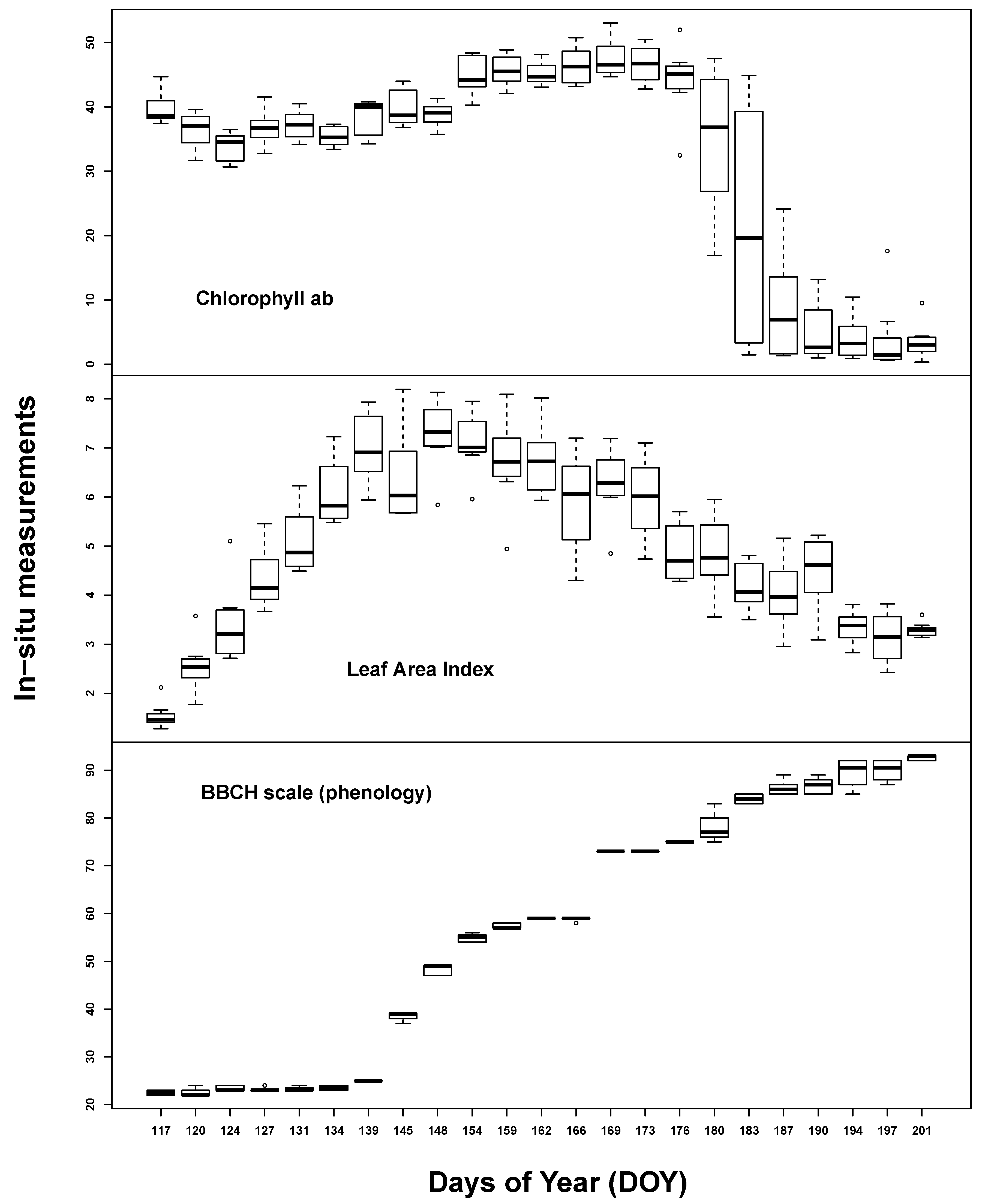
Temporal plant biophysical properties were dominated by plant phenology. While there was also some effect of the different implemented water treatments at the end of the measurement period, soil influence seemed to be almost negligible. All
in situ measurements varied considerably over the course of the seasonal evolution (see
Figure 1). Chlorophyll content was high throughout the early to middle growing stages (35–45 µg/cm
2) until the start of ripening. LAI steadily increased up to 7 m
2/m
2 until ear appearance, followed by slow, steady decline. BBCH measurements covered most of the barley macro-stages: tillering (20–29), stem elongation (30–39), ear appearance (40–49), heading (50–59), flowering (60–69), fruit development (70–79), fruit ripening (80–89) and senescence (90+).
3.1.2. Field
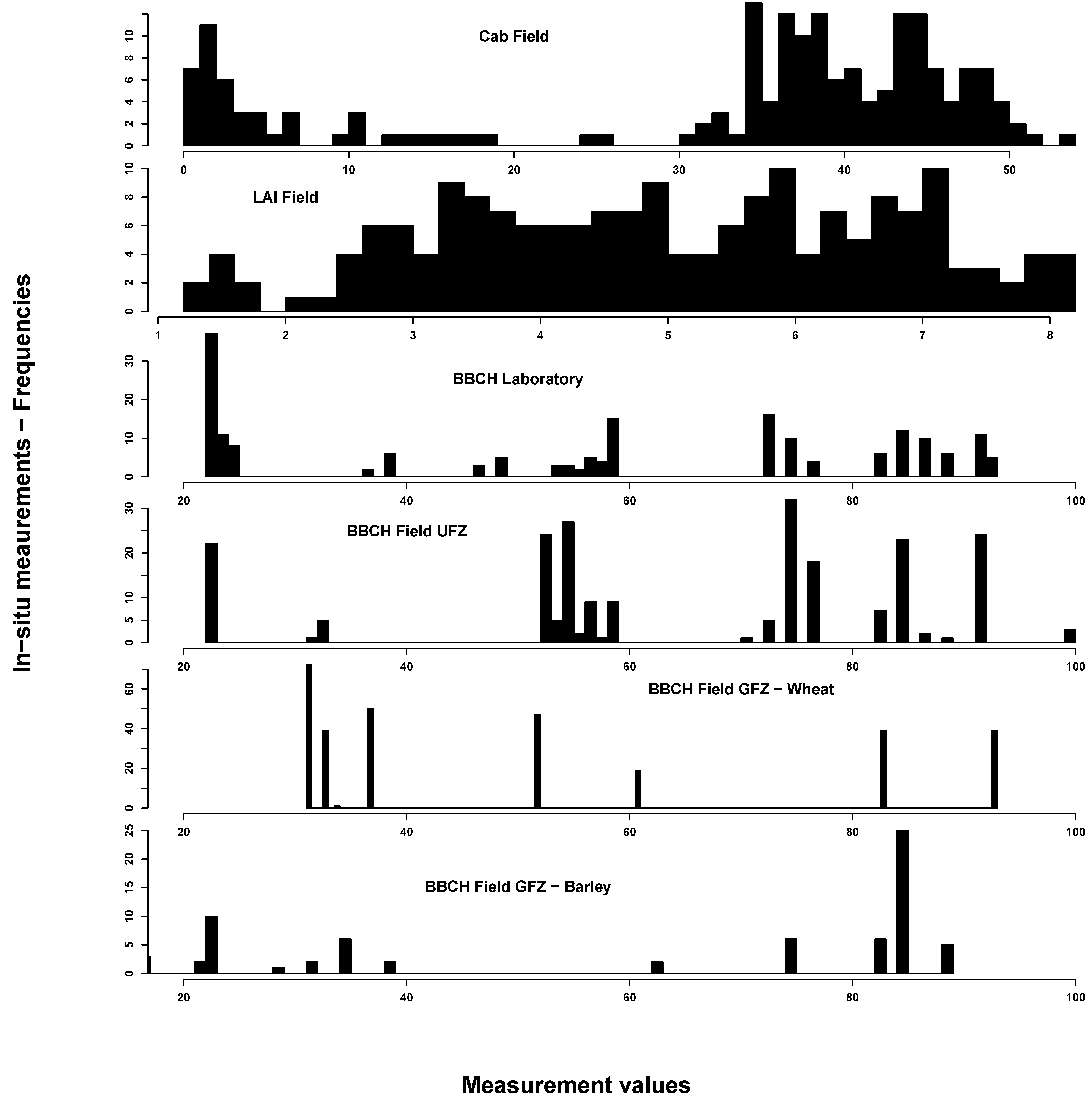
In situ measurements exhibited the spectrum of eco-physiological values for chlorophyll, LAI and BBCH, considering that most of the vegetation period was covered by measurements (see
Figure 2). Most C
ab values could be found around 40 and around 5 µg/cm
2. This reflects the typical bimodal C
ab distribution over a crop vegetation period with moderate to high values until the start of ripening and subsequent very low values. LAI was normally distributed between 1 and 8 m
2/m
2. BBCH measurements covered most of the macro-stages. There were, however, some differences between GFZ and UFZ measurements: GFZ measurements did not include BBCH stages below 30 and between 62 and 82 for wheat, but generally more measurements between BBCH 30 and 40.
Figure 1.
Summary of the in situ laboratory measurements: chlorophyll content (µg/cm2) (top), Leaf Area Index (m2/m2) (middle) and phenological measurements (Growth stages of mono-and dicotyledonous plants, BBCH scale) (bottom).
Figure 1.
Summary of the in situ laboratory measurements: chlorophyll content (µg/cm2) (top), Leaf Area Index (m2/m2) (middle) and phenological measurements (Growth stages of mono-and dicotyledonous plants, BBCH scale) (bottom).
Figure 2.
Summary of the in situ field measurements: chlorophyll content (µg/cm2) (top), Leaf Area Index (m2/m2) (second from top) and phenological measurements from the German Research Center for Geosciences (GFZ) and Helmholtz Centre for Environmental Research-UFZ (UFZ) Growth stages of mono-and dicotyledonous plants (BBCH) scale) (bottom two). For comparison, the laboratory BBCH measurements are also shown (middle)
3.2. PROSAIL Simulations
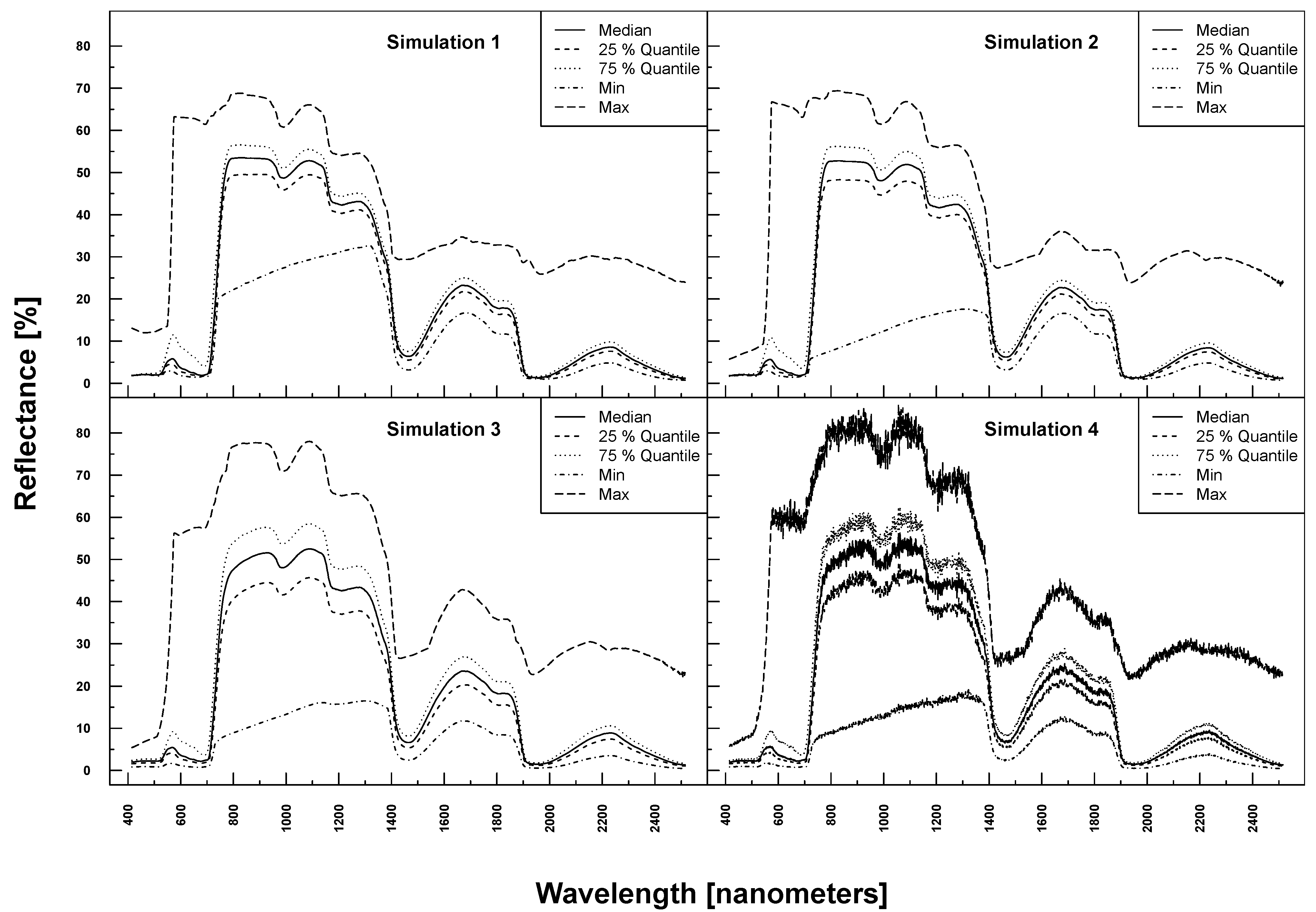
PROSAIL simulated spectra varied considerably in shape and magnitude within and between Simulations 1–4 (see
Figure 3). The more parameters were varied, the higher the variation at each wavelength. Simulation 3, for example, exhibited higher maximum and lower minimum reflectances over the full spectrum compared to Simulation 1. The added noise and bias clearly translated into the reflection profiles of Simulation 4.
Figure 3.
PROSAIL simulated spectral profiles (summary statistics over 10,000 simulations). Variation of basic biophysical and structural parameters (Simulation 1) (top left), variation of additional soil parameters (Simulation 2) (top right), variation of all parameters (Simulation 3) (bottom left) and variation of all parameters + additional noise and bias (Simulation 4) (bottom right).
3.3. Random Forest Prediction
All vegetation parameters in Simulations 1 and 2 (additional soil influence) could be derived precisely (
R2 near one, see
Table 3). In Simulation 3, where all biophysical and structural model variables were varied, prediction accuracy was still very high for C
ab, but lower when deriving LAI. Added noise and bias (Simulation 4) did not affect RF performance. RF prediction accuracy was lower on laboratory data with
R2 values between 0.80 and 0.94. Deduction of phenological phases based on ASD measurements could be performed at a similar level as respective C
ab and LAI estimates.
Table 3.
RF prediction accuracy (R-squared and cross-validation) on simulated, laboratory and field data (FR using the first five PCA components). RF predictions on laboratory and field data were based on 100 runs with randomly varying training datasets (median thereof). Cross-validation was 10-fold. BBCH prediction based on GFZ field measurements is shown for wheat (first value) and barely (second value) separately.
| Dataset | R2 Cab | MAE Cab | R2 LAI | MAE LAI | R2 BBCH | MAE BBCH |
|---|
| Simulation 1 | 0.99 | 2.09 | 0.98 | 0.56 | - | - |
| Simulation 2 | 0.99 | 2.37 | 0.97 | 0.63 | - | - |
| Simulation 3 | 0.98 | 3.21 | 0.88 | 1.10 | - | - |
| Simulation 4 | 0.98 | 3.23 | 0.89 | 0.88 | - | - |
| Laboratory data | 0.94 | 4.66 | 0.80 | 0.91 | 0.91 | 8.01 |
| Field data UFZ | 0.89 | 6.94 | 0.89 | 0.65 | 0.80 | 10.72 |
| Field data GFZ | - | - | - | - | 0.85/0.88 | 9.87/12.07 |
RF prediction accuracy (
R2) was generally at a similar level for laboratory and field-based measurements: C
ab and BBCH at a slightly lower level and LAI at a slightly higher level (see
Table 3). Phenological stages could be derived with similar predictive power for the two independent field measurement sets (UFZ and GFZ). Prediction accuracy was just marginally affected by the species observed,
i.e., wheat or barley (see
Table 3). The number of UFZ field measurements with single crops was too low to allow for a robust comparison. RF predictions on the complete datasets were similar (
R2 0.80 for UFZ and 0.85 for GFZ field measurements). MAE of C
ab estimates increased when more complexity was introduced in PROSAIL simulations and furthermore for laboratory and field measurements. In contrast, MAE of LAI estimates decreased for Simulation 4 and also for all ASD measurements, despite decreasing
R2.
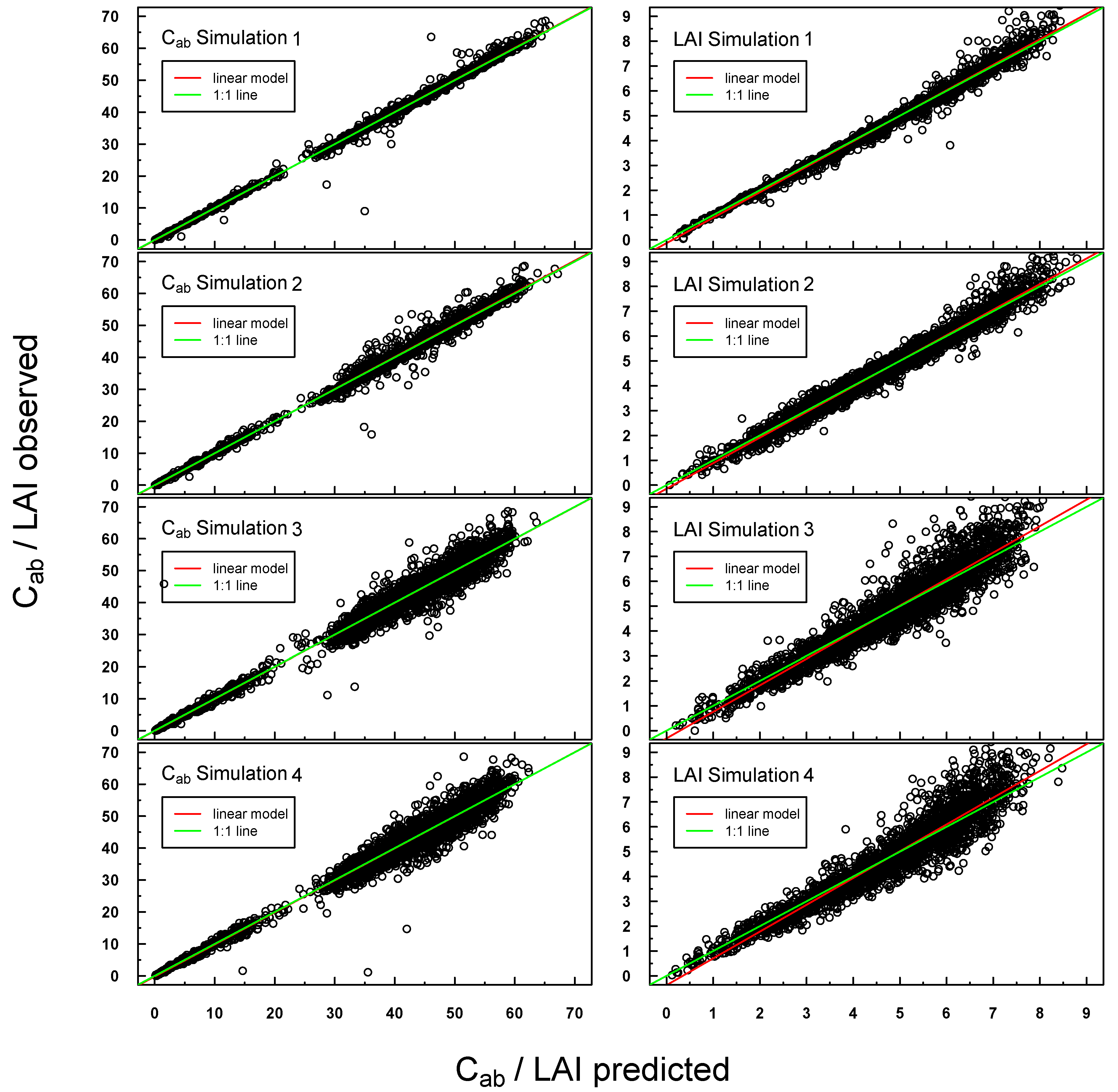
Predicted
vs. observed C
ab/LAI values for PROSAIL Simulations 1–4 were highly positively linearly correlated (see
Figure 4). Scattering increased slightly for Simulations 3 and 4, especially at higher LAI values. A small offset could be detected for LAI Simulations 3 and 4.
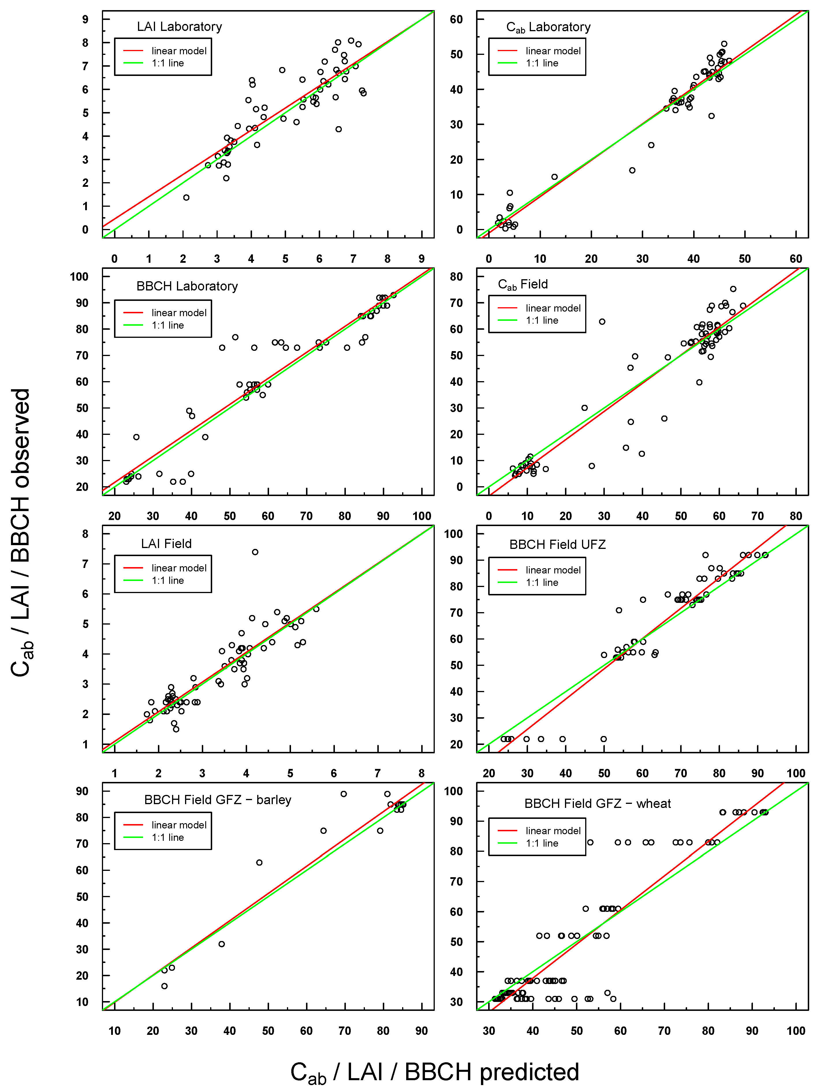
Predicted
vs. observed values for
in situ laboratory and field measurements were also highly positively linearly correlated (see
Figure 5). Scattering was generally more pronounced with respect to Simulations 1–4, but the respective linear regressions were still very close to the ideal 1:1 line.
Figure 4.
Scatterplot of predicted vs. measured Cab/LAI for PROSAIL Simulations 1–4. The respective linear regression model is indicated with a red line and the “ideal” 1:1 relationship with a green line. In the case of a congruent linear regression and a 1:1 line, the former is superimposed by the latter.
Figure 5.
Scatterplot of predicted vs. observed values for all laboratory and field in situ measurements (Cab, LAI, BBCH). The respective linear regression model is indicated with a red line and the “ideal” 1:1 relationship with a green line. In the case of a congruent linear regression and a 1:1 line, the former is superimposed by the latter.
3.4. Important Wavelengths
RF also provides a measure of internally assigned importance/weights for predicting variables (wavelengths) based on the grown tree structure. Here, we extracted for each run the 20 most important wavelengths (a single run for simulated data and 100 for ASD measurements). Because RF results for ASD measurements are based on 100 runs, selected important wavelengths are presented as frequencies. The most prominent spectral regions selected as predictor variables just varied slightly between Simulations 1–4 and ASD measurements regressing on C
ab (see
Table 4 and
Figure 6,
Figure 7,
Figure 8,
Figure 9 and
Figure 10). However, laboratory and field measurements also included spectral regions from NIR and SWIR. Selected wavelengths when regressing on LAI did generally vary more, also within PROSAIL simulations.
Table 4.
Summary of most important spectral regions (in nm) selected by RF for simulated, laboratory and field-based hyperspectral profiles. GFZ collected BBCH stages only for spectral field measurements.
Table 4.
Summary of most important spectral regions (in nm) selected by RF for simulated, laboratory and field-based hyperspectral profiles. GFZ collected BBCH stages only for spectral field measurements.
| Dataset | Cab | LAI | BBCH |
|---|
| Simulation 1 | 700–720 | 750, 1140, 1270, 1870 | - |
| Simulation 2 | 700–720 | 1,140, 1270, 1870 | - |
| Simulation 3 | 680–715 | 930, 960, 1700, 1870 | - |
| Simulation 4 | 680–715 | 950, 1450, 1700, 1870 | - |
| Laboratory data | 680–710, 2300 | 715, 810–910, 1100–1300 | 700, 1450, 2300 |
| Field data UFZ | 680–810, 1150, 1430, 2300 | 450–500, 750–950, 1200 | 700, 780, 1300, 2300 |
| Field data GFZ | - | - | 400, 700, 780, 1300, 1450, 2000 |
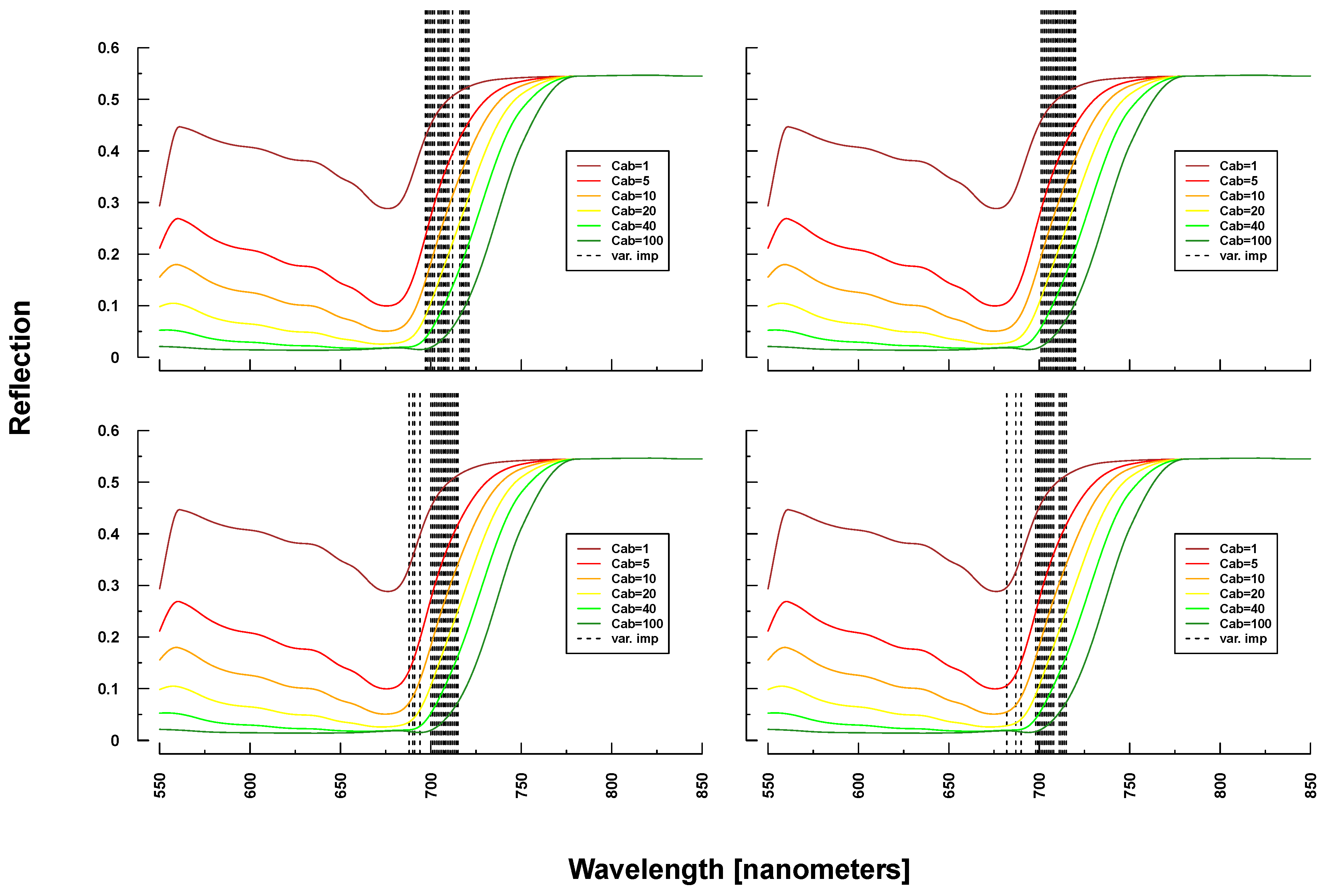
Figure 6.
Identified important wavelengths (according to RF) for predicting chlorophyll content based on PROSAIL simulations. A single run was performed with a randomly selected training dataset. Identified important wavelengths are plotted as vertical lines. Colored lines indicate PROSAIL simulated spectral profiles with changing Cab parameterization between 1 and 100 g/m2 (y-axis). For all simulations, the same spectraare plotted. Variation of basic biophysical and structural parameters (Simulation 1) (top left), variation of additional soil parameters (Simulation 2) (top right), variation of all parameters (Simulation 3) (bottom left)and variation of all parameters + additional noise and bias (Simulation 4) (bottom right).
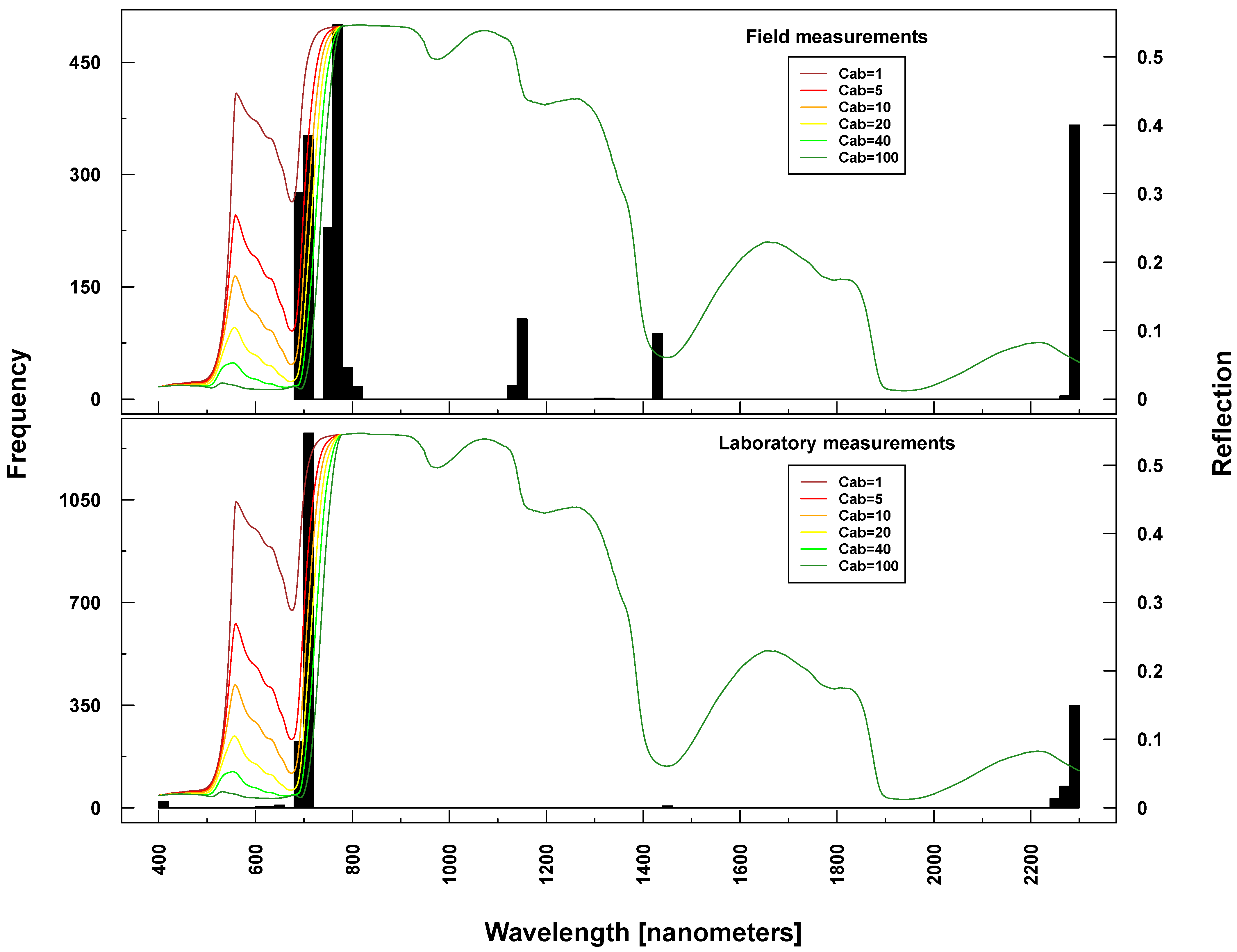
Selected important wavelengths for C
ab prediction originated consistently from the VIS and red edge (rapid reflectance change of vegetation in the NIR), covering the spectral regions between 680 and 810 nm (vertical lines or bars in
Figure 6 and
Figure 7). This is the spectral region that is most affected when changing C
ab parameters values in PROSAIL simulations (colored lines in respective Figures). In the case of ASD measurements, also wavelengths at 2300 nm (laboratory and field) and at 1150/1430 nm (field only) were selected (
Figure 7), where changing C
ab content has little or no influence on simulated spectra according to PROSAIL.
Figure 7.
Identified important wavelengths (according to RF) for predicting chlorophyll content based on ASD laboratory (bottom) and field measurements (top). One hundred RF runs were performed with randomly selected training datasets. Identified important wavelengths are plotted as frequencies (y-axis). Lines indicate PROSAIL simulated spectral profiles with changing Cab parameterization between 1 and 100 g/m2 (z-axis).
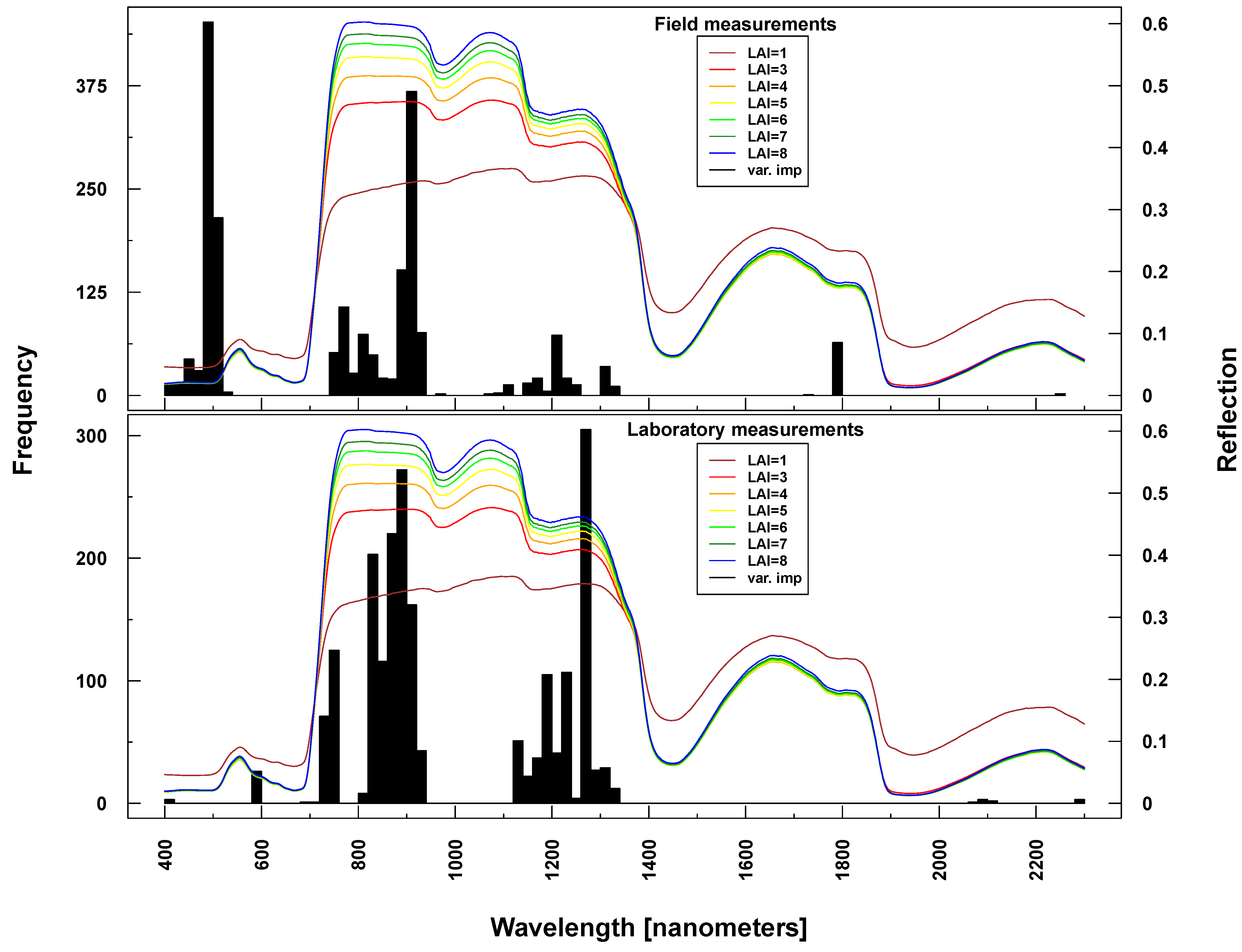
Important variables for LAI prediction of PROSAIL simulations were consistently selected from the NIR and SWIR (vertical lines or bars in
Figure 8 and
Figure 9). This is in line with PROSAIL simulations based on changing LAI parameterization where the spectral region between 800 and 1200 nm is mostly affected. However, within these spectral regions, selected wavelengths changed considerably between Simulations 1 and 4. Please notice that changes below LAI = 2 can affect the complete electromagnetic spectrum between 400 and 2500 nm. Important wavelengths for deriving LAI from laboratory and field measurements were primarily situated in the spectral region 700–1300 nm, hence excluding wavelengths >1400 nm, which were selected from all PROSAIL simulations. Field measurement-based predictions also included wavelengths around 500 nm (
Figure 9).
Figure 8.
Identified important wavelengths (according to RF) for predicting LAI based on PROSAIL simulations. A single run was performed with a randomly selected training dataset. Identified important wavelengths are plotted as vertical lines. Colored lines indicate PROSAIL simulated spectral profiles with changing LAI parameterization between 1 and 9 m2/m2(y-axis). For all simulations, the same spectra are plotted. Variation of basic biophysical and structural parameters (Simulation 1) (top left), variation of additional soil parameters (Simulation 2) (top right), variation of all parameters (Simulation 3) (bottom left) and variation of all parameters + additional noise and bias (Simulation 4) (bottom right).
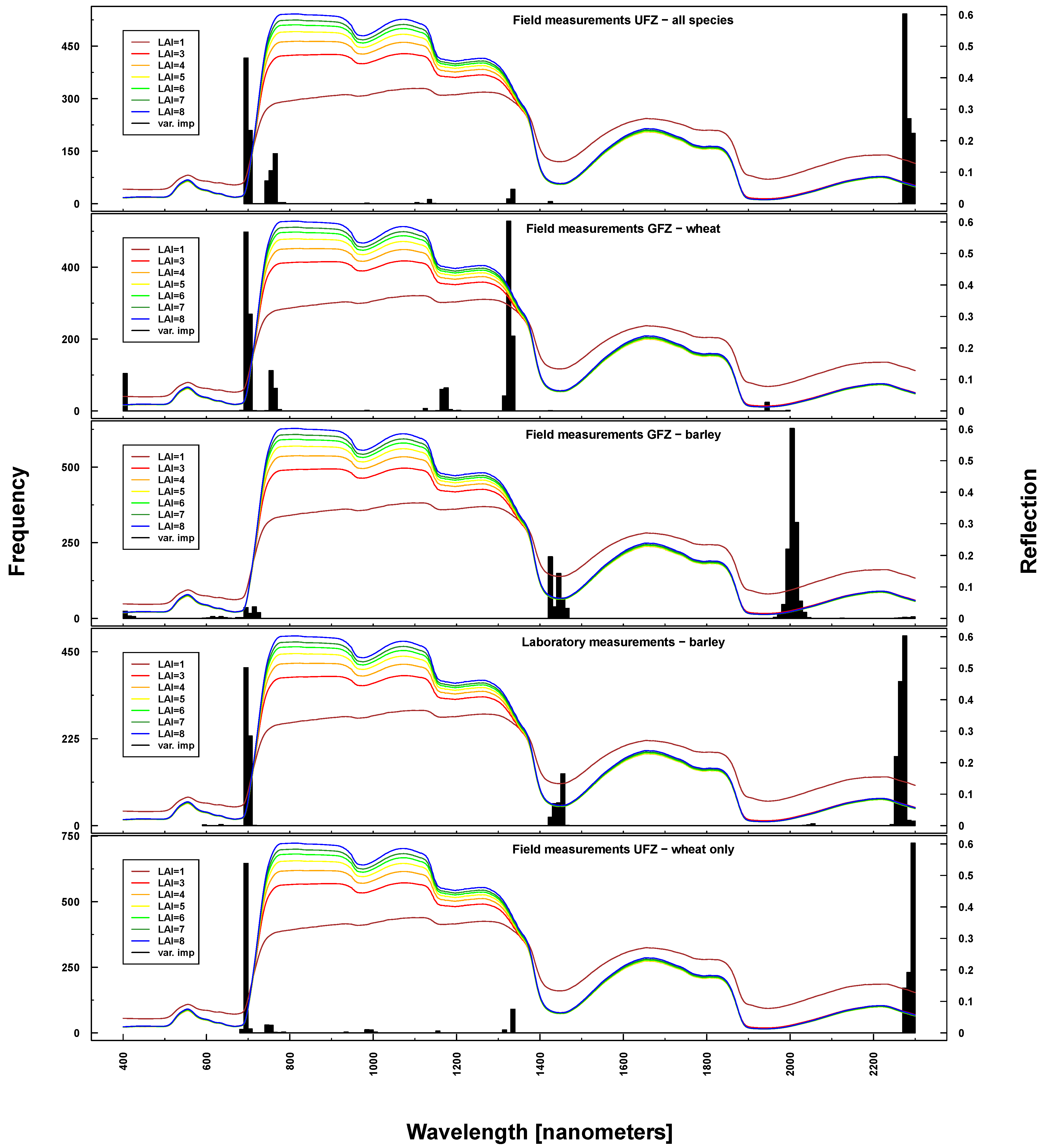
Important wavelengths for deriving phenological phases were considered to be in the red edge (~700 nm), at 1330 nm, 1450 nm, 2000 nm and 2200 nm (see
Figure 10). Differences between UFZ laboratory and field measurements mainly concerned wavelengths around 1450 nm (not selected for field measurements). This spectral region was included when using GFZ barley field measurements, but not GFZ wheat field measurements. Here, the spectral region around 1330 nm was selected as important, which features only marginally in UFZ wheat field measurements.
Figure 9.
Identified important wavelengths (according to RF) for predicting LAI based on ASD laboratory (bottom) and field measurements (top). One hundred RF runs were performed with randomly selected training datasets. Identified important wavelengths are plotted as frequencies (y-axis). Lines indicate PROSAIL simulated spectral profiles with changing LAI parameterization between one and nine.
Figure 10.
Identified important wavelengths (according to RF) for predicting BBCH based on ASD laboratory (bottom), UFZ field measurements (top) and GFZ field measurements (middle). One hundred RF runs were performed with randomly selected training datasets. Identified important wavelengths are plotted as frequencies (y-axis). Lines indicate PROSAIL simulated spectral profiles with changing LAI parameterization between one and nine.
4. Discussion
RF prediction accuracy was very high for simulated data. The more influencing variables were kept constant in the simulation process, the better the derivation of vegetation physiological status. C
ab estimates were excellent, even within more complex data structures,
i.e., varying all PROSAIL biophysical and structural vegetation parameters + additional noise and bias (
R2 = 0.98), while
R2 values were a bit lower for LAI (0.89). RF performance decreased slightly on laboratory and field data, but including field-based measurements had no detrimental affect on prediction accuracies. The goodness of chlorophyll estimates were comparable with other studies [
35,
36,
37].
The most important selected variables (wavelengths/spectral regions) changed marginally between PROSAIL Simulations 1–4 and also between simulations, laboratory and field measurements when regressing on C
ab. Moderate changes of prediction variables were found when regressing on LAI or BBCH; changes between laboratory and field measurements were not more pronounced than within PROSAIL simulations. Despite selecting, on average, prediction variables from appropriate spectral regions, prior knowledge of physical processes is crucial. Plant’s biophysical properties constitute different proportions of measured reflectance dependent on the wavelength. Bacour
et al. [
38], for example, quantified the relative contributions of all canopy variables on reflectance used in PROSAIL,
i.e., the percentage of the total variance explained by a given variable. Results indicate that chlorophyll content accounts for ~60% of the reflectance variation in the VIS (400–700 nm). In the NIR (700–1100 nm), the most important variables are the average leaf angle and the leaf area index, which contribute equally to reflectance [
15].
Consequently, one would expect that the selection of important variables for estimating chlorophyll and LAI refers to the spectral regions mentioned above. Overall, selected wavelengths for C
ab and LAI correspond well with the above-mentioned sensitivity analysis conducted by [
38,
39], independent of whether simulated, laboratory or field data were used. Bands considered to be most important for modeling C
ab were very similar to those identified in simulated data. LAI prediction was primarily based on wavelengths in the NIR and SWIR, spectral regions dominated by the vegetation’s structural components [
15,
23]. Wavelengths considered to be most important by RF corresponded well with the findings of other studies [
37,
40].
A few sets of important variables included wavelengths from spectral regions with no physical relationship to the response variable (for example, 2300 nm for predicting C
ab/BBCH). Furthermore, selected wavelengths were not always consistent between implemented simulations, especially concerning LAI (compare Simulations 1/2
vs. 3/4). This might be caused by the fact that parameter sets with different values can exhibit the same reflection profile: the complex variable interaction influencing NIR and SWIR seems to impede variable selection from that spectral region. Furthermore, some wavelengths most likely provide information that has only a mathematical-statistical relationship. Machine learning methods, including RF, sometimes show tendencies of overfitting [
41]. That means the algorithm in use actually fits background noise rather than selecting biophysically meaningful prediction variables. This would also explain the slightly improved LAI prediction for Simulation 4 compared to Simulation 3.
The devolution of barley phenological growth stages (BBCH scale) is intimately connected with C
ab and LAI changes: high chlorophyll content throughout the early to middle growing stages and a sharp decrease with the start of ripening, while LAI steadily increases until ear appearance, followed by slow, steady decline. A simple RF model can predict the BBCH scale well based on
in situ C
ab and LAI measurements alone (
R2 = 0.74). Consequently, one would expect the selected important wavelengths originating from two spectrally different groups (VIS and NIR). This was primarily the case, but waveband selection also included the far SWIR region for both field and laboratory measurements. Noticeable is the selection of the spectral region around 1450 nm as an important predictor when deriving phenological stages for GFZ barley field measurements and UFZ barley laboratory measurements. It seems that geometric properties specific to barley, e.g., the long awn, are behind this selection. Differences between spectral regions selected from GFZ and UFZ wheat measurements are likely to originate from the varying coverage of BBCH stages during data acquisition. However, also, other factors, such as crop management (row spacing, orientation) might affect variable selection from different datasets, as found by [
42] when discriminating crop types.
Possibly limiting factors of the implemented approach can be divided into four groups as follows.
- (1)
RF limitations related to hyperspectral data: Many highly correlated predictor variables were used to model vegetation status by the RF algorithm; variable importance often included groups of adjacent wavelengths. Furthermore, wavelengths that are not physically related to the investigated response, but that may contain unique information content (like the 2300-nm spectral region), can be selected as important prediction variables. Nevertheless, most predictors were selected from biophysically meaningful spectral areas. Given the RF preceding feature reduction, future studies might have to include a set of prominent machine learning/kernel methods. Wavelengths consistently selected by all applied methods could then be assumed as robust prediction variables. Even though PCA is often used for feature reduction of hyperspectral data [
43], there are other methods already available that sometimes outperform PCA, such as maximum noise fraction transformation (MNF, [
44]) or non-parametric weighted feature extraction (NWFE, [
45,
46]. Still, the Hughes’ phenomenon is likely to affect many pre-processing and data mining methods [
47,
48].
- (2)
Limitations of inverse modeling: Naturally, the retrieval of biophysical variables from remote sensing data is in any case affected by the problem that several biophysical and structural vegetation characteristics have an impact on the same spectral regions. As the inversion of RTM is generally an under-determined problem, knowledge on the distribution of model parameters is helpful [
15], which requires one to determine as many parameters required by the used RTM as possible.
- (3)
Limitations of PROSAIL. Although PROSAIL is an extensively used and tested RTM [
15], a simple one-dimensional model like this has limitations. The canopy description by the means of LAI and an LIDF should be mentioned here. A possible improvement might be the use of a more sophisticated, but also more complicated, three-dimensional model, where vegetation structure can be better represented [
6]. However, subsequently, the estimation of many more vegetation structure parameters would be necessary. Obviously, summer barley canopy structure changed substantially between growth, maturation and senescence phases. Describing these canopy structure changes is difficult based on parameter mean values. The collected ASD spectra over the whole measurement period could not be fully represented in the model parameterization. Especially, the appearance of ears/awns specific to summer barley cannot be described within PROSAIL. Investigating different growing stages separately could improve prediction accuracy, but limits transferability to field or airborne data acquisitions.
- (4)
Limitations of
in situ measurements: The selection of unexpected wavelengths by RF for LAI might originate from difficulties in providing a representative sample size of
in situ observations, despite intensive sampling efforts. Furthermore, C
ab, LAI and BBCH
in situ data are affected by measurement uncertainties. For example, indices based on hyperspectral reflectance measurements have been found to derive C
ab more robustly than SPAD measurements [
49,
50]. Finally, it was observed that there is an important influence of the phenological phase on the appearance of summer barley spectra, which is difficult to capture by PROSAIL model parameterization. Furthermore, the effect of ears specific to summer barley on ASD measurements could be detected, as already mentioned.
Advantages:
- (1)
RF was shown to be a robust prediction method for simulated, laboratory and field data. A performance decrease between simulated and measured hyperspectral signatures has to be expected given measuring inaccuracies (both in situ and hyperspectral); for example, inherent slight diversions from nadir positions performing ASD measurements even with strict measurement protocols. Temporal sampling in the laboratory, even on identical barley plots, was very dense compared to field measurements. In this respect, slight decreases in prediction performance are negligible indicating that environmental conditions, e.g., changing illumination, seem to have only minor influences. Prediction differences between the two independent field datasets of GFZ and UFZ can most likely be attributed to the different coverage of BBCH stages and different acquisition procedures, but are still comparably close.
- (2)
The inclusion of multi-temporal hyperspectral data with different growth stages (and physiological status’) posed no limitations on RF prediction performance. Most studies evaluated machine learning techniques on hyperspectral data acquisitions with very homogeneous growth stages. Here, we could show similar prediction accuracies with all phenological growth stages included. Likewise, [
51] used crop ASD measurements at different scales and different BBCH stages for successfully predicting biomass.
- (3)
Variables for predictive RF models were in most cases selected from biophysically meaningful spectral regions. Wavelengths selected for LAI prediction do vary more because changing LAI affects a considerable part of VNIR and SWIR, even extending into VIS at low LAI values.
- (4)
No extensive parameter tuning is required when applying RF on hyperspectral data. Changing “mtry” or “ntree” had little effect on prediction quality and robustness. The proposed settings of “mtry = 1000” and “ntree = 700” should also be applicable to other studies dealing with hyperspectral data. This is in contrast to other machine learning or kernel methods, such as in support vector regression or kernel ridge regression, where extensive parameter tuning, with the risk of overfitting, is standard procedure. Chan and Paelinckx [
52] also found RF to be a fast, stable and robust method when deriving land use classes.
5. Conclusions
This study tested whether the impediment to derive vegetation parameters from hyperspectral signatures at consistently high levels stems from their high dimensionality, (changing) environmental factors, such as illumination conditions, or the uncertainty of in situ measurements. Therefore, vegetation parameters were extracted from a unique combination of three independent datasets: simulated signatures, laboratory and field measurements covering a complete vegetation period combined with respective in situ measurements. Consequently, the applicability of machine learning methods, like randomForest, for deriving the plant physiological status from hyperspectral signatures was investigated. Based on PROSAIL simulated data, the potential of this approach, which is able to represent also non-linear relations and interactions between variables, could be demonstrated. randomForest was almost not affected by artificially introduced noise and bias in data: high accuracy estimates for chlorophyll content (R2 = 0.98) and LAI (R2 = 0.89). Despite shortcomings when simulating crop hyperspectral signatures at certain phenological growth stages, this study could still demonstrate the usefulness of a radiative transfer model, like PROSAIL, to assess statistical approaches on simulated hyperspectral data: when testing against simulated signatures, the truth is already known, i.e., one is able to discriminate between randomForest performance and measurement uncertainties or changing environmental conditions. This in contrast to most approaches, where machine learning methods are tested against measurements only.
In a next step, the transferability of the approach to laboratory and field data was investigated. For a full vegetation period of summer barley, RF performance was good, but accuracies were not as high as for simulated spectra (Cab: R2 = 0.94/LAI: R2 = 0.80/BBCH: R2 = 0.91). Prediction accuracies for field measurements were at a similar level demonstrating randomForest’s applicability also with datasets influenced by changing environmental conditions. Nevertheless, unexpected wavelengths were selected as important, specifically for Cab and BBCH estimation. These unexpected wavelengths, however, were not restricted to field, but included also laboratory measurements. The selection of different important predictors might be due to (i) insufficient sample sizes of laboratory and field data or (ii) PROSAIL model limitations. Providing a representative sample size of in situ observations is still considered to be one of the major difficulties despite intensive sampling efforts.
RandomForest performed well on hyperspectral data with underlying high phenological complexity. Applying this methodology on single principal growth stages would improve prediction accuracy, but was not investigated here. As a result, randomForest can be used for predicting plant physiological status on multi-temporal and also airborne hyperspectral data (given precise atmospheric/geometric correction). Mixed pixels should not have a detrimental effect on prediction accuracy if these consist of different crop types: BBCH estimates in this study could be performed at a similar level, including a single or different crop type(s). However, predictor variables were not consistently selected from similar spectral regions using randomForest. Most likely, varying plant geometry between crop types (wheat vs. barley) and also different data acquisition times (different geometry and chemical composition) cause this varying selection. Decreasing performance between simulated and laboratory and field data indicates that in situ measurement uncertainties are the most limiting factor when deriving bio-physical plant properties. This is despite some PROSAIL limitations simulating ASD, like data for all phenological stages.
Future studies should implement and test a set of prominent machine learning/kernel methods, especially for variable selection. Wavelengths consistently selected by all applied methods could then be assumed robust prediction variables. Geometrical plant properties at certain growth stages impede appropriate variable selection based on one method only. Consequently, we recommend a more intense use of 3D simulation models that account for changing geometrical properties dependent on phenological stage. This is even more important when airborne or satellite data over larger areas are analyzed, where exact phenological stages are not precisely known. Application on simulated spectral profiles (2D or 3D models) offers more insights regarding the general evaluation of a machine learning method and facilitates the interpretation of the results obtained. Regarding spectral field measurements, we recommend intense spectral sampling with many repetitions and averaging to minimize measurements inaccuracies.
Benefits from using hyperspectral remote sensing data could, next to the demonstrated randomForest potential, be shown, as well. Although their high dimensionality and autocorrelation complicates the interpretation of selected important variables, they offer extended information content compared to multispectral data. Allowing for the derivation of biophysical and structural vegetation parameters with high temporal and/or spatial resolution covering large areas, remote sensing data are of special importance for the ecosystem modeling science community.
Acknowledgments
The authors would like to acknowledge Ines Merbach, Renate Hintz and Sabine Straßenburg for cultivating and attending the analyzed crop in the Bad Lauchstädt laboratory. Many thanks also to Marion Pause, Gundula Schulz, Gudrun Schuhmann and Steffen Lehmann for the intense measurement efforts during 2009–2013.
Author Contributions
Daniel Doktor designed this study, analyzed the data, performed the radiative transfer modeling, feature reduction and wrote the manuscript together with Martin Thurner. Martin Thurner also significantly contributed to the data analysis and set-up the modeling part. Angela Lausch set-up the laboratory measurement design. Daniel Spengler contributed to the GFZ dataset and edited the manuscript.
Conflicts of Interest
The authors declare no conflict of interest.
References
- Baret, F.; Houles, V.; Guerif, M. Quantification of plant stress using remote sensing observations and crop models: The case of nitrogen management. J. Exp. Bot. 2007, 58, 869–880. [Google Scholar] [CrossRef] [PubMed]
- Migliavacca, M.; Meroni, M.; Busetto, L.; Colombo, R.; Zenone, T.; Matteucci, G.; Manca, G.; Seufert, G. Modeling gross primary production of agro-forestry ecosystems by assimilation of satellite-derived information in a process-based model. Sensors 2009, 9, 922–942. [Google Scholar] [CrossRef] [PubMed] [Green Version]
- Boegh, E.; Thorsen, M.; Butts, M.B.; Hansen, S.; Christiansen, J.S.; Abrahamsen, P.; Hasager, C.B.; Jensen, N.O.; van der Keur, P.; Refsgaard, J.C.; et al. Incorporating remote sensing data in physically based distributed agro-hydrological modeling. J. Hydrol. 2004, 287, 279–299. [Google Scholar] [CrossRef]
- Raupach, M.R.; Rayner, P.J.; Barrett, D.J.; DeFries, R.S.; Heimann, M.; Ojima, D.S.; Quegan, S.; Schmullius, C.C. Model-data synthesis in terrestrial carbon observation: Methods, data requirements and data uncertainty specifications. Glob. Chang. Biol. 2005, 11, 378–397. [Google Scholar] [CrossRef]
- Govender, M.; Dye, P.J.; Weiersbye, I.M.; Witkowski, E.T.F.; Ahmed, F. Review of commonly used remote sensing and ground-based technologies to measure plant water stress. Water SA 2009, 35, 741–752. [Google Scholar] [CrossRef]
- Dorigo, W.A.; Zurita-Milla, R.; de Wit, A.J.W.; Brazile, J.; Singh, R.; Schaepman, M.E. A review on reflective remote sensing and data assimilation techniques for enhanced agroecosystem modeling. Int. J. Appl. Earth Observ. Geoinf. 2007, 9, 165–193. [Google Scholar] [CrossRef]
- Breiman, L. Random forests. Mach. Learn. 2001, 45, 5–32. [Google Scholar] [CrossRef]
- Ismail, R.; Mutanga, O. A comparison of regression tree ensembles: Predicting Sirex noctilio induced water stress in Pinus patula forests of KwaZulu-Natal, South Africa. Int. J. Appl. Earth Observ. Geoinf. 2010, 12, S45–S51. [Google Scholar] [CrossRef]
- Prasad, A.M.; Iverson, L.R.; Liaw, A. Newer classification and regression tree techniques: Bagging and random forests for ecological prediction. Ecosystems 2006, 9, 181–199. [Google Scholar] [CrossRef]
- Cutler, D.R.; Edwards, T.C.; Beard, K.H.; Cutler, A.; Hess, K.T. Random forests for classification in ecology. Ecology 2007, 88, 2783–2792. [Google Scholar] [CrossRef] [PubMed]
- Lawrence, R.L.; Wood, S.D.; Sheley, R.L. Mapping invasive plants using hyperspectral imagery and Breiman Cutler classifications (RandomForest). Remote Sens. Environ. 2006, 100, 356–362. [Google Scholar] [CrossRef]
- Chan, J.C.W.; Paelinckx, D. Evaluation of Random Forest and Adaboost tree-based ensemble classification and spectral band selection for ecotope mapping using airborne hyperspectral imagery. Remote Sens. Environ. 2008, 112, 2999–3011. [Google Scholar] [CrossRef]
- Jacquemoud, S.; Baret, F. Prospect—A model of leaf optical-properties spectra. Remote Sens. Environ. 1990, 34, 75–91. [Google Scholar] [CrossRef]
- Verhoef, W. Light-scattering by leaf layers with application to canopy reflectance modeling—The sail model. Remote Sens. Environ. 1984, 16, 125–141. [Google Scholar] [CrossRef]
- Jacquemoud, S.; Verhoef, W.; Baret, F.; Bacour, C.; Zarco-Tejada, P.J.; Asner, G.P.; Francois, C.; Ustin, S.L. PROSPECT plus SAIL models: A review of use for vegetation characterization. Remote Sens. Environ. 2009, 113, S56–S66. [Google Scholar] [CrossRef]
- Lichtenthaler, H.K. Chlorophylls and carotenoids—Pigments of photosynthetic biomembranes. Methods Enzymol. 1987, 148, 350–382. [Google Scholar]
- Vohland, M.; Mader, S.; Dorigo, W. Applying different inversion techniques to retrieve stand variables of summer barley with PROSPECT plus SAIL. Int. J. Appl. Earth Observ. Geoinf. 2010, 12, 71–80. [Google Scholar] [CrossRef]
- Markwell, J.; Osterman, J.C.; Mitchell, J.L. Calibration of the Minolta SPAD-502 leaf chlorophyll meter. Photosynth. Res. 1995, 46, 467–472. [Google Scholar] [CrossRef] [PubMed]
- Bleiholder, H.; Weber, E.; Hess, M.; Wicke, H.; van den Boom, T.; Lancashire, P.; Buhr, L.; Hack, H.; Klose, R.; Stauss, R. Growth Stages of Mono- and Dicotyledonous Plants, BBCH Monograph; Federal Biological Research Centre for Agriculture and Forestry: Berlin/Braunschweig, Germany, 2001; p. 158. [Google Scholar]
- Feret, J.B.; Francois, C.; Asner, G.P.; Gitelson, A.A.; Martin, R.E.; Bidel, L.P.R.; Ustin, S.L.; le Maire, G.; Jacquemoud, S. PROSPECT-4 and 5: Advances in the leaf optical properties model separating photosynthetic pigments. Remote Sens. Environ. 2008, 112, 3030–3043. [Google Scholar] [CrossRef]
- Verhoef, W.; Jia, L.; Xiao, Q.; Su, Z. Unified optical-thermal four-stream radiative transfer theory for homogeneous vegetation canopies. IEEE Trans. Geosci. Remote Sens. 2007, 45, 1808–1822. [Google Scholar] [CrossRef]
- Baret, F.; Hagolle, O.; Geiger, B.; Bicheron, P.; Miras, B.; Huc, M.; Berthelot, B.; Nino, F.; Weiss, M.; Samain, O.; et al. LAI, fAPAR and fCover CYCLOPES global products derived from VEGETATION—Part 1: Principles of the algorithm. Remote Sens. Environ. 2007, 110, 275–286. [Google Scholar] [CrossRef] [Green Version]
- Jacquemoud, S. Inversion of the prospect + sail canopy reflectance model from aviris equivalent spectra—Theoretical-study. Remote Sens. Environ. 1993, 44, 281–292. [Google Scholar] [CrossRef]
- Weiss, M.; Baret, F. Evaluation of canopy biophysical variable retrieval performances from the accumulation of large swath satellite data. Remote Sens. Environ. 1999, 70, 293–306. [Google Scholar] [CrossRef]
- Breiman, L.; Friedman, J.; Olshen, R.; Stone, C. Classification and Regression Trees; Chapman and Hall: London, UK, 1984. [Google Scholar]
- Liaw, A.; Wiener, M. Package “randomForest”. Breiman and Cutler’s Random Forests for Classification and Regression. 2014. Available online: http://cran.r-project.org/web/packages/randomForest/randomForest.pdf (accessed on 28 October 2014).
- R Core Team. R Core Team; R Foundation for Statistical Computing: Vienna, Austria. Available online: http://www.R-project.org/ (accessed on 5 November 2014).
- Gislason, P.; Benediktsson, J.; Sveinsson, J. Random Forests for land cover classification. Pattern Recognit. Lett. 2006, 27, 294–300. [Google Scholar] [CrossRef]
- Waske, B.; Benediktsson, J.A.; Arnason, K.; Sveinsson, J.R. Mapping of hyperspectral AVIRIS data using machine-learning algorithms. Can. J. Remote Sens. 2009, 35, S106–S116. [Google Scholar] [CrossRef]
- Okujeni, A.; van der Linden, S.; Jakimow, B.; Rabe, A.; Verrelst, J.; Hostert, P. A comparison of advanced regression algorithms for quantifying urban land cover. Remote Sens. 2014, 6, 6324–6346. [Google Scholar] [CrossRef]
- Dalponte, M.; Orka, H.O.; Gobakken, T.; Gianelle, D.; Naesset, E. Tree species classification in boreal forests with hyperspectral data. IEEE Trans. Geosci. Remote Sens. 2013, 51, 2632–2645. [Google Scholar] [CrossRef]
- Schwieder, M.; Leitao, P.J.; Suess, S.; Senf, C.; Hostert, P. Estimating fractional shrub cover using simulated EnMAP data: A comparison of three machine learning regression techniques. Remote Sens. 2014, 6, 3427–3445. [Google Scholar] [CrossRef]
- Castaings, T.; Waske, B.; Benediktsson, J.A.; Chanussot, J. On the influence of feature reduction for the classification of hyperspectral images based on the extended morphological profile. Int. J. Remote Sens. 2010, 31, 5921–5939. [Google Scholar] [CrossRef]
- Fassnacht, F.E.; Neumann, C.; Foerster, M.; Buddenbaum, H.; Ghosh, A.; Clasen, A.; Joshi, P.K.; Koch, B. Comparison of feature reduction algorithms for classifying tree species with hyperspectral data on three central European test sites. IEEE J. Sel. Top. Appl. Earth Observ. Remote Sens. 2014, 7, 2547–2561. [Google Scholar]
- Atzberger, C.; Guerif, M.; Baret, F.; Werner, W. Comparative analysis of three chemometric techniques for the spectroradiometric assessment of canopy chlorophyll content in winter wheat. Comput. Electr. Agric. 2010, 73, 165–173. [Google Scholar] [CrossRef]
- Jarmer, T. Spectroscopy and hyperspectral imagery for monitoring summer barley. Int. J. Remote Sens. 2013, 34, 6067–6078. [Google Scholar] [CrossRef]
- Verrelst, J.; Alonso, L.; Rivera Caicedo, J.P.; Moreno, J.; Camps-Valls, G. Gaussian process retrieval of chlorophyll content from imaging spectroscopy data. IEEE J. Sel. Top. Appl. Earth Observ. Remote Sens. 2013, 6, 867–874. [Google Scholar] [CrossRef]
- Bacour, C.; Baret, F.; Jacquemoud, S. Information content of HyMap hyperspectral imagery. In Proceedings of the 1st International Symposium on Recent Advances in Quantitative Remote Sensing, Valencia, Spain, 16–20 September 2002; Sobrino, J., Ed.; University of Valencia: Valencia, Spain, 2002; pp. 503–508. [Google Scholar]
- Bacour, C.; Jacquemoud, S.; Tourbier, Y.; Dechambre, M.; Frangi, J.P. Design and analysis of numerical experiments to compare four canopy reflectance models. Remote Sens. Environ. 2002, 79, 72–83. [Google Scholar] [CrossRef]
- Li, X.; Zhang, Y.; Bao, Y.; Luo, J.; Jin, X.; Xu, X.; Song, X.; Yang, G. Exploring the best hyperspectral features for LAI estimation using partial least squares regression. Remote Sens. 2014, 6, 6221–6241. [Google Scholar] [CrossRef]
- Dormann, C.F.; Elith, J.; Bacher, S.; Buchmann, C.; Carl, G.; Carre, G.; Marquez, J.R.G.; Gruber, B.; Lafourcade, B.; Leitao, P.J.; et al. Collinearity: A review of methods to deal with it and a simulation study evaluating their performance. Ecography 2013, 36, 27–46. [Google Scholar] [CrossRef]
- Galvão, L. Crop type discrimination using hyperspectral data. In Hyperspectral Remote Sensing of Vegetation; Thenkabail, P.S., Lyon, J.G., Huete, A., Eds.; CRC Press, Taylor and Francis Group: New York, NY, USA, 2012; Chapter 17; pp. 397–422. [Google Scholar]
- Thenkabail, P.S.; Lyon, J.G.; Huete, A. Advances in hyperspectral remote sensing of vegetation and agricultural crops. In Hyperspectral Remote Sensing of Vegetation; Thenkabail, P.S., Lyon, J.G., Huete, A., Eds.; CRC Press, Taylor and Francis Group: New York, NY, USA, 2012; Chapter 1; pp. 3–29. [Google Scholar]
- Green, A.; Berman, M.; Switzer, P.; Craig, M. A transformation for ordering multispectral data in terms of image quality with implications for noise removal. IEEE Trans. Geosci. Remote Sens. 1988, 26, 65–74. [Google Scholar]
- Falco, N.; Benediktsson, J.A.; Bruzzone, L. A study on the effectiveness of different independent component analysis algorithms for hyperspectral image classification. IEEE J. Sel. Top. Appl. Earth Observ. Remote Sens. 2014, 7, 2183–2199. [Google Scholar] [CrossRef]
- Kuo, B.; Landgrebe, D. Nonparametric weighted feature extraction for classification. IEEE Trans. Geosci. Remote Sens. 2004, 42, 1096–1105. [Google Scholar] [CrossRef]
- Hughes, G. On the mean accuracy of statistical pattern recognizers. IEEE Trans. Inf. Theory 1968, 14, 55–63. [Google Scholar] [CrossRef]
- Thenkabail, P.S.; Gumma, M.K.; Teluguntla, P.; Mohammed, I.A. Hyperspectral remote sensing of vegetation and agricultural crops. Photogramm. Eng. Remote Sens. 2014, 80, 697–709. [Google Scholar]
- Richardson, A.; Duigan, S.; Berlyn, G. An evaluation of noninvasive methods to estimate foliar chlorophyll content. New Phytol. 2002, 153, 185–194. [Google Scholar] [CrossRef]
- Gitelson, A. Non-destructive estimation of foliar pigment (chlorophylls, carotenoids, and anthocyanins) contents: Evaluating a semi-analytical three-band model. In Hyperspectral Remote Sensing of Vegetation; Thenkabail, P.S., Lyon, J.G., Huete, A., Eds.; CRC Press, Taylor and Francis Group: New York, NY, USA, 2012; Chapter 6; pp. 141–166. [Google Scholar]
- Gnyp, M.L.; Bareth, G.; Li, F.; Lenz-Wiedemann, V.I.S.; Koppe, W.; Miao, Y.; Hennig, S.D.; Jia, L.; Laudien, R.; Chen, X.; et al. Development and implementation of a multiscale biomass model using hyperspectral vegetation indices for winter wheat in the North China Plain. Int. J. Appl. Earth Observ. Geoinf. 2014, 33, 232–242. [Google Scholar] [CrossRef]
- Chan, J.C.W.; Paelinckx, D. Evaluation of Random Forest and Adaboost tree-based ensemble classification and spectral band selection for ecotope mapping using airborne hyperspectral imagery. Remote Sens. Environ. 2008, 112, 2999–3011. [Google Scholar] [CrossRef]
© 2014 by the authors; licensee MDPI, Basel, Switzerland. This article is an open access article distributed under the terms and conditions of the Creative Commons Attribution license (http://creativecommons.org/licenses/by/4.0/).


