1. Introduction
In the last 30 years, Earth observation satellites have played a central role in monitoring, understanding and quantifying land cover-land use dynamics and environmental processes. Consistent and continuous datasets of Earth observations from coarse-resolution sensors [
1] have been extensively used and enabled the study of the phenological cycles of vegetation [
2,
3,
4,
5,
6], responses of vegetation dynamics to climate change [
7], inter- and intra-annual variations of ecosystem productivity [
8], land cover dynamics and biophysical variables at regional, continental and global scales [
9,
10]. With the advent of the century, an improved generation of moderate- and coarse-resolution instruments, such as SPOT-VEGETATION, Medium Resolution Imaging Spectrometer (MERIS) and Moderate Resolution Imaging Spectroradiometer (MODIS), has enhanced our capabilities for monitoring vegetation dynamics [
9,
11,
12], biophysical variables [
13,
14,
15,
16], ecosystem variables [
17,
18,
19] and land surface disturbances [
20,
21].
At higher spatial resolutions, the Landsat satellite series, starting in 1972, has accumulated the oldest temporal record of space-based Earth observations. Landsat provides 30-m spatial resolution imagery with a 16-day revisit period over a 183 × 170-km extent and represents a considerable improvement in spatial detail from previous sensors, allowing the identification of land surface dynamics previously undetectable from space. The opening of the Landsat archive [
22] creates new opportunities for temporal studies of land surfaces at higher spatial resolution. Taking advantage of these opportunities and in response to a need to expose variations of land surfaces at finer spatial detail, a number of studies have used temporal series of Landsat data to analyze vegetation trends and the dynamics of phenology [
23,
24], as well as forest disturbance and recovery patterns [
25,
26,
27,
28]. More recently, Zhu and Woodcock [
29] demonstrated, over a temperate site of the United States, a continuous change detection and classification method that uses historical and present Landsat imagery. Yan and Roy [
30] presented an automated computational methodology to extract agricultural crop fields over large regions from time series of Landsat data. However, the potential of Landsat for continuous monitoring of land surfaces is still limited by its revisit period and the availability of cloud-free surface observations [
31]. Some studies overcome this problem using cloud-free composites from multiyear Landsat images as representative of a given epoch [
32,
33,
34]. Yet, rather than a truly continuous monitoring capability, this approach provides Earth observation snapshots not necessarily suitable for monitoring surface processes associated with intra-annual variations, such as agriculture cycles, or gradual processes, such as post-fire vegetation recovery.
The combination of high-revisit moderate- and medium-spatial resolution from Landsat-like sensors has the potential to improve the capabilities for land surface monitoring. Moderate- and medium-spatial resolution sensors have been already integrated for regional and continental mapping initiatives [
32,
35,
36]. A limited number of studies explore the integration of sensors with different spatial and temporal resolutions for continuous monitoring of land surfaces. For instance, several methods have been proposed to simulate Landsat images at dates for which cloud-free imagery is not available. These methods rely on models of various complexity based on the relationships between moderate- and fine-resolution images coincident in time. Gao
et al. [
37] developed an empirical fusion technique that blends 500-m MODIS and Landsat surface reflectance using an initial Landsat image and a pair of MODIS images. Subsequently, Walker
et al. [
38] applied this approach to explore dryland forest phenology. Hilker
et al. [
39] proposed a method to monitor land cover changes in forested landscapes at fine resolution based on a fine-resolution land cover change map and a time series of 500-m MODIS Normalized Difference Vegetation Index (NDVI) images. Within a similar framework, Zhu
et al. [
40] enhanced Gao’s approach, implementing a spectral unmixing approach to improve the retrieval of heterogeneous pixels. Roy
et al. [
41] developed a semi-empirical fusion approach using MODIS/bidirectional reflectance distribution function (BRDF) albedo and Landsat surface reflectance to generate precedent or antecedent synthetic Landsat images. Unlike the previous methods, Roy
et al. [
41] accounted for the directional dependence of surface reflectance via Sun-sensor geometry. Zurita
et al. [
42] and Amorós-López
et al. [
43] have presented a spectral unmixing method to generate time series of vegetation indices at fine resolution using MERIS and Landsat imagery together with ancillary land use information. In general, these fusion methods successfully retrieve individual synthetic fine-resolution scenes, provided a pair of coincident in time moderate- and fine-resolution images are not too far apart. However, for a given site, the quality of their simulation degrades when the simulated scene is further in time from the reference pair, as the initial assumptions of the models become weaker and land surfaces change. None of these methods provide information for the uncertainty of the simulated images.
In this paper, we propose a data assimilation method that simulates time series of medium-resolution synthetic images built from existing medium-resolution imagery and time series of moderate resolution imagery. The method implements a Kalman filter (KF) algorithm in which information from observing systems and models are combined optimally to minimize residuals. Within the framework of a state-space statistical model, the approach incorporates uncertainties in the calculation of the synthetic images and quantifies the amount of knowledge about future outcomes [
44]. The inclusion of uncertainty information in the calculation process makes this method robust and flexible enough to work with datasets of suboptimal quality and still achieve results comparable to those reported in the literature. Rather than retrieving single synthetic images, it also enables the production of full temporal sequences of synthetic images. The method is demonstrated for the predictions of synthetic Landsat NDVI at 16-day time steps. Within the KF framework, it uses the available Landsat images as observations and the time series of 250-m NDVI MODIS (MOD13Q1) as the source of a model of the seasonal evolution of land surfaces. The method is applied on a per-pixel basis, does not require tuning parameters and has the flexibility to work independently of the number of existing medium resolution images. For simplicity, this paper applies the term “medium resolution” for Landsat and similar sensors and “moderate resolution” for MODIS and equivalent instruments.
3. Methods
This paper proposes a data assimilation approach based on a Kalman filter algorithm [
52] simulates time series of medium-resolution synthetic images assimilating information from medium-resolution imagery and time series of moderate resolution imagery. KF is a recursive inference algorithm that integrates observations, models and their respective uncertainties to estimate the state of a process minimizing the mean of the squared errors [
53,
54]. Kalman filter algorithms have been applied to correct atmospheric effects in satellite images [
55], image fusion of multisource images [
56,
57,
58,
59], integrate remote sensing data and ecosystem models in a number of studies to retrieve soil temperature [
60], surface BRDF parameters [
61], soil moisture [
62], change detection [
63], ecosystem productivity [
64] or monitoring crop phenology [
65].
KF retrieves the states of a process based on a combination of present measurements, a linear state-transition model and the respective uncertainties of these elements.
where
xk−1 and
xk are the model estimates in the previous and present state, respectively;
A represents the transition model linking
xk and
xk−1;
zk is the observation at a given state;
w and
v are Gaussian random variables that represent the process noise
N(0,
Q) and measurement noise
N(0,
R), respectively;
H relates the state to the observation
zk. The KF algorithm is implemented in two steps. First (time update), the linear state-transition model propagates the estimate of the previous state and its uncertainty to provide prior estimates of the present state of the model (3) and its uncertainty (4).
where
is the posterior estimate of the variable in the previous state;
is the prior estimate of the present estate;
is the posterior uncertainty of the previous state; and
the prior uncertainty for the present state. In a second step (measurement update), prior estimates (5) and their uncertainties (6) are updated with new observations via a linear combination of the prior model estimate and a weighted difference between the observations and the prior estimate of the model state. The weighs are defined by the “Kalman gain” (
K) (7).
where
is the posterior estimate of the state. Large measurement noise (
R) results in low Kalman gains, which give more weight to the model process. Conversely, large process covariance (
P) results in high Kalman gains and more weight for the new measurements.
KF can be applied in two different inference problems: “filtering” and “smoothing”. Filtering involves calculating the estimate of a certain state based on a partial sequence of outputs. This sequence can include precedent or subsequent states for forward and backward recursion, respectively [
52,
66]. Smoothing estimates a state based on data from both previous and later times and requires combining a forward and a backward recursion of the KF algorithm [
67]. Thus, while filtering is relevant in an online learning sense, in which current conditions are to be estimated by the currently available data, smoothing applies in a
post hoc sense, where there is a need to optimally interpolate past events in a time series.
3.1. Kalman Filter Implementation
In this study, a Kalman filter recursive algorithm was implemented to simulate synthetic NDVI images and estimate their respective uncertainties at 30-m spatial resolution at 16-day time steps with the goal of improving the temporal consistency of Landsat NDVI time series. The implementation of the KF algorithm required the definition of a set of observations and an underlying linear state-transition model. The available NDVI Landsat images within the period of study were defined as observations (
Figure 2). The number of available NDVI Landsat scenes and the time gaps between scenes varied for each site (
Table 2). A preliminary analysis showed that the average standard deviation of the NDVI values within 3 × 3 kernels ranged from 4.5% and 6.8% of the central NDVI value in the study sites. Based on these figures, a normally distributed noise of mean zero and standard deviation 5% of the NDVI pixel value was determined for all sites. This value accounted for potential misregistration between MODIS and Landsat images after a preliminary analysis of the variability of pixel values within a 3 × 3-pixel neighborhood in the NDVI Landsat scenes. Other potential sources of errors, such as instrumental and pre-processing errors, were not considered in this study.
The transition model was defined as an ensemble of two submodels. At each state, the outputs of both submodels were combined to reduce the uncertainty and provide a more robust estimate [
68], with uncertainties representing a measure of the confidence about a future state. The first submodel provides a general trajectory of the NDVI values to characterize the temporal vegetation dynamics in the areas of study [
61]. While there are a number of alternatives to generate local or pixel-based seasonal trends using ancillary and contextual information [
37,
42], in this study, we implement a single seasonal trend for each site. Adopting a single seasonal trend is an obvious simplification of the real world in which each vegetated land cover has a unique seasonal trajectory that fluctuates within the limits set by regional environmental factors, such as temperature, precipitation and photoperiod. However, despite its constraints, a transition model based on a single seasonal trend serves to test whether the inclusion of uncertainties can, despite the use of a simpler model, retrieve comparable results in the estimation of the synthetic images. This approach also ensures the flexibility to implement the method in the absence of ancillary information and maintain computationally efficiency. The phenological trajectories were extracted from the seasonal NDVI patterns obtained from MODIS 16-day composites (MOD13Q1). To minimize the impact of ephemeral clouds that are not masked out in the MODIS composites, the original 16-day NDVI composites were smoothed by applying a moving average with a five-composite temporal window for each pixel in the images. The model defined the trajectories as piece-wise regressions. Each piece was defined by the linear regression between NDVI MODIS values at consecutive states built from a sufficiently large subset of randomly selected pixels within the scene that preserved the computational efficiency of the routine (
N = 10,000). The slope and intercept of the linear regressions are used to obtain the
a priori estimate at state
k from Submodel (1),
where
is the
a priori estimate at state
k from Submodel (1) and
is the
a posteriori estimate from state
k − 1. Both
a and
b are the slope and intercept of the linear regression of NDVI MODIS values at consecutive states between time steps
k − 1 and
k. The uncertainties associated with each step of the submodel were calculated as the standard error of the linear regression at each step. A unique seasonal trajectory was defined for each study site.
The second submodel captured the relationship between MODIS and Landsat NDVI pixel values and provides an additional constraint to the seasonal trajectories of the first submodel. Rather than explicitly accounting for non-linearities induced by factors, such as viewing and illumination angles, pixel adjacency effects and radiometric differences between sensors, this submodel implicitly accounts for potential image noise and non-linearities that could result in weaker relationships between the pair of images and contribute larger uncertainties to the Kalman filter model. To do so, a linear regression model was built for each pair of concurrent MODIS composite and Landsat image. The slope and intercept of the linear regression are used to obtain the
a priori estimate at state
k from Submodel (2),
where
is the
a priori estimate at stake
k from Submodel (2). In this equation,
c and
d are the slope and intercept of the linear regression of NDVI MODIS and Landsat values at a given state
k. A Landsat scene was considered concurrent to a given MODIS composite when its acquisition date fell within the first and last acquisition dates of the composite. As with the first submodel, the linear regression was built from a subset of randomly selected pixels (
N = 10,000). For a given state, the linear regression of the last state with concurrent MODIS and Landsat NDVI images was applied. The uncertainties of the submodel were calculated as the standard error of the linear regression.
Assuming the estimates of the two submodels for the same time step are both independent and Gaussian, the transition model (A) at each time step is their joint estimate, calculated as:
where
,
,
denote the
a priori estimates of the state variable at time
k from the first and second submodels and the combined model, respectively; and
,
,
are the corresponding
a priori variances.
The initial state of the model is crucial to build accurate time series of NDVI values. The highest resolution available NDVI estimate was used for the initialization of the model. If a Landsat image was available for the first state (x0), it was taken as the initial step, and the uncertainty (Q0) was estimated as the standard deviation of the pixels within the image. If a Landsat image did not exist for the first state, the first MODIS NDVI composite defined the initial state within the period of study. The uncertainty associated with the MODIS NDVI composite was defined as the standard deviation of the pixels within the composite.
The KF algorithm was implemented in both filtering and smoothing modes. The smoothing mode estimates of the temporal sequences of medium-resolution NDVI images required the combination of forward and backward KF recursions applying equations equivalent to [
10] and [
11]:
where
,
and
denote the posterior estimates at state
t in forward, backward and combined mode, respectively;
PFk,
PBk and
PFBk, are the uncertainties at state
k in forward, backward and combined mode, respectively;
Rk is the measurement uncertainty at state
k. MATLAB software (MATLAB 2011a, The MathWorks, Inc., Natick, MA, United States) was used to code and implement the Kalman filter algorithm.
3.2. Accuracy Analysis
Accuracies were evaluated by comparing concurrent synthetic NDVI images against Landsat NDVI images not used as observations in the production of temporal sequences of synthetic images. For each pair of concurrent synthetic and validation Landsat images, prediction residuals at the pixel level were computed as the difference between the predicted and observed NDVI:
where
Δpredk is the residual at pixel level, NDVIsyn
k is the pixel value in the synthetic image and NDVIobs
k is the pixel value in the validation image. Additionally, as in Roy
et al. [
21], the residual difference between Landsat NDVI images at different acquisition dates (
k,
k +
i) was computed as:
where Δ
tempk,k+i is the temporal residual at the pixel level,
NDVIk+i and
NDVIk are the pixel values in the time steps
k +
i and
k, respectively, and
k +
i corresponds to the acquisition date of NDVIobs
k. Image level residuals were calculated as the average of residuals at the pixel level from a random sample of pixels within the image (
N = 10,000). After initial tests, this sample size proved to be representative of the whole image, while improving the efficiency of the computations. To allow the comparison of image-level residuals between sites, normalized residuals at the image level were computed as:
where
and
are the normalized predicted and normalized temporal residual at the image level, respectively. In a reliable synthetic NDVI image, the prediction residuals should be smaller than temporal residuals [
21].).
Figure 2.
Flow chart of the Kalman filter approach. At each time step, the transition model, A, projects the estimate from a previous state (time update). The time update combines the estimates of Submodels 1 and 2,
and , respectively, to produce a single a priori estimate, . If available, a Landsat observation, Zk, provides a new estimate for the state (measurement update). The final estimate of the state, , is the weighted average of the time update (transition model) and the measurement update (Landsat observation), with the weights inversely proportional to their respective uncertainties. If a new Landsat observation is not available, the estimate of the state at that time step is solely the result of the measurement update from previous time step. The model is alternatively run in forward and backward mode (filtering mode) and the corresponding estimates subsequently combined (smooth mode).
To evaluate the performance of the method for the generation of complete temporal sequences of synthetic NDVI images, a Monte Carlo framework was implemented and nearly 1000 simulations were run for each site. At each simulation, the number of Landsat observations and their position within the temporal sequence were randomly selected from the existing Landsat images. For each temporal sequence generated, image level residuals and normalized residuals were calculated using as validation the Landsat images not used in the process. Mean residuals for each temporal sequence were estimated from the image-level residuals within the sequence.
For a given site, the accuracy of a temporal sequence is a function of the number of observations and their position within the sequence. To evaluate the sensitivity of the residuals to the number of observations used in the generation of the temporal sequence, summary statistics (mean and standard deviation) were derived from temporal sequence residuals built with the same number of Landsat observations. These calculations were separately implemented for temporal sequences generated in forward, backward and combined recursions.
4. Results
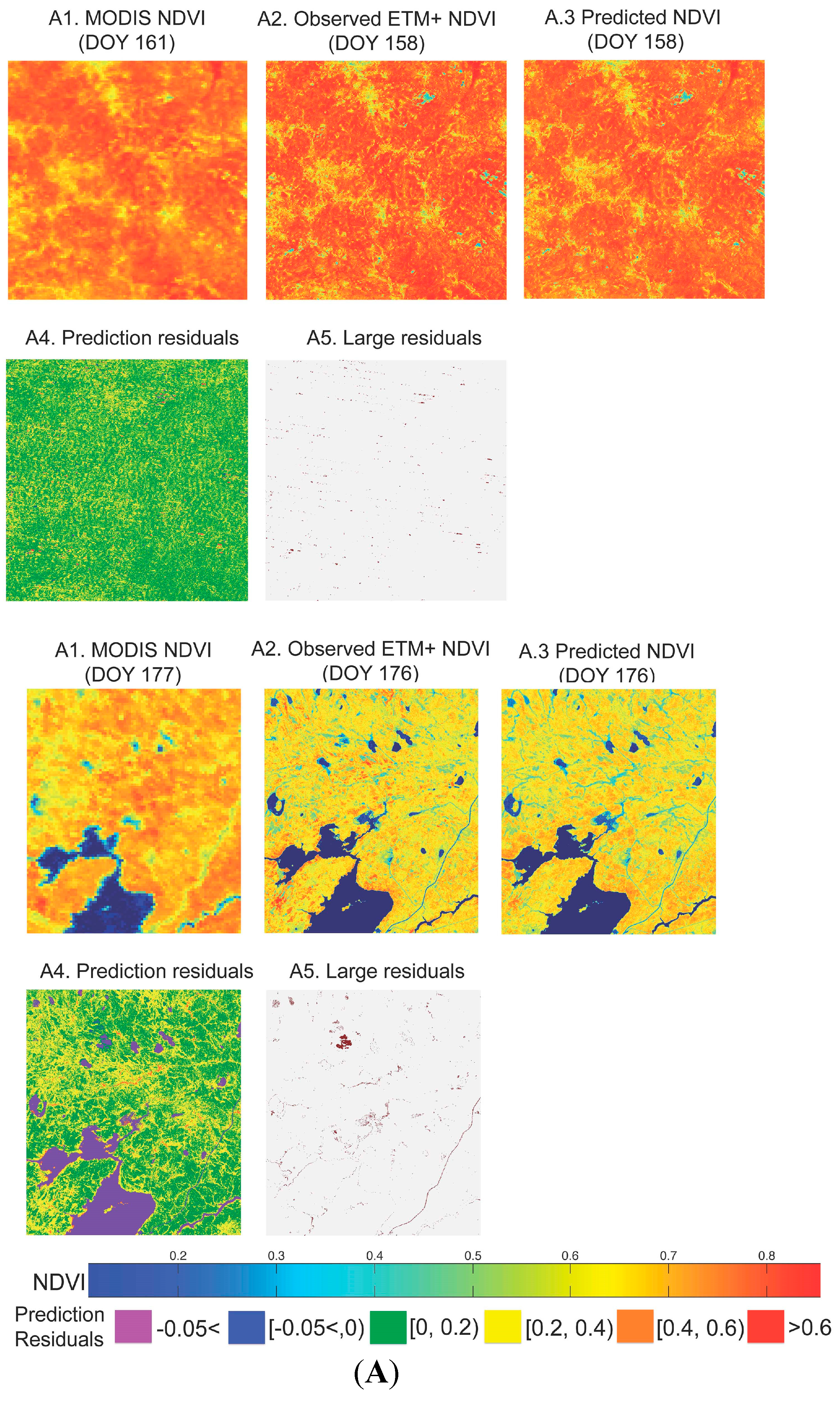
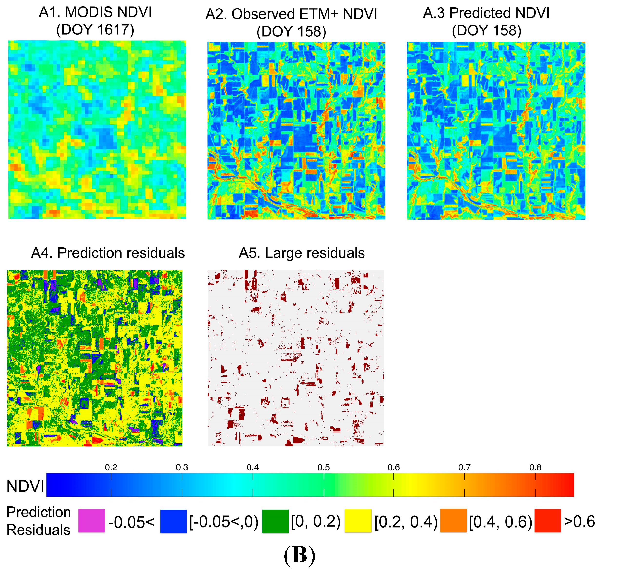
Figure 3a,b shows subsets of synthetic NDVI images generated one time step (
t +
1) from a Landsat observation and the concurrent Landsat NDVI validation, NDVI MODIS and residual images. For each site, there is a significant gain in spatial detail between the synthetic images and the 250-m NDVI MODIS images. Visually, the validation and synthetic NDVI images are highly similar in spatial structure. Low predicted residuals dominate the subset images, with values between zero and 0.25 dominating the images (
Figure 4 and
Figure 5). Large residuals (larger than 0.25) are limited and associated with linear features, such as watercourses at the Arizona and Manitoba sites, and areas of rough relief, such as deep valleys at the Arizona site. At the Kansas site, while still dominated by low residuals, larger residuals occur in areas where, because of agricultural management, there are rapid land surface changes.
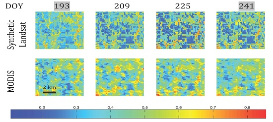
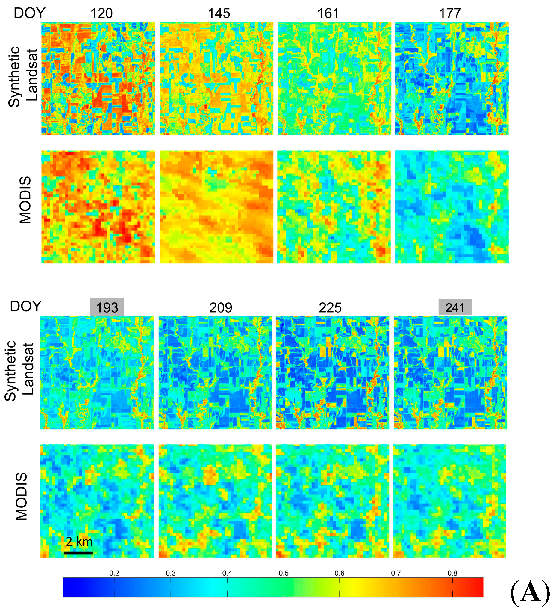
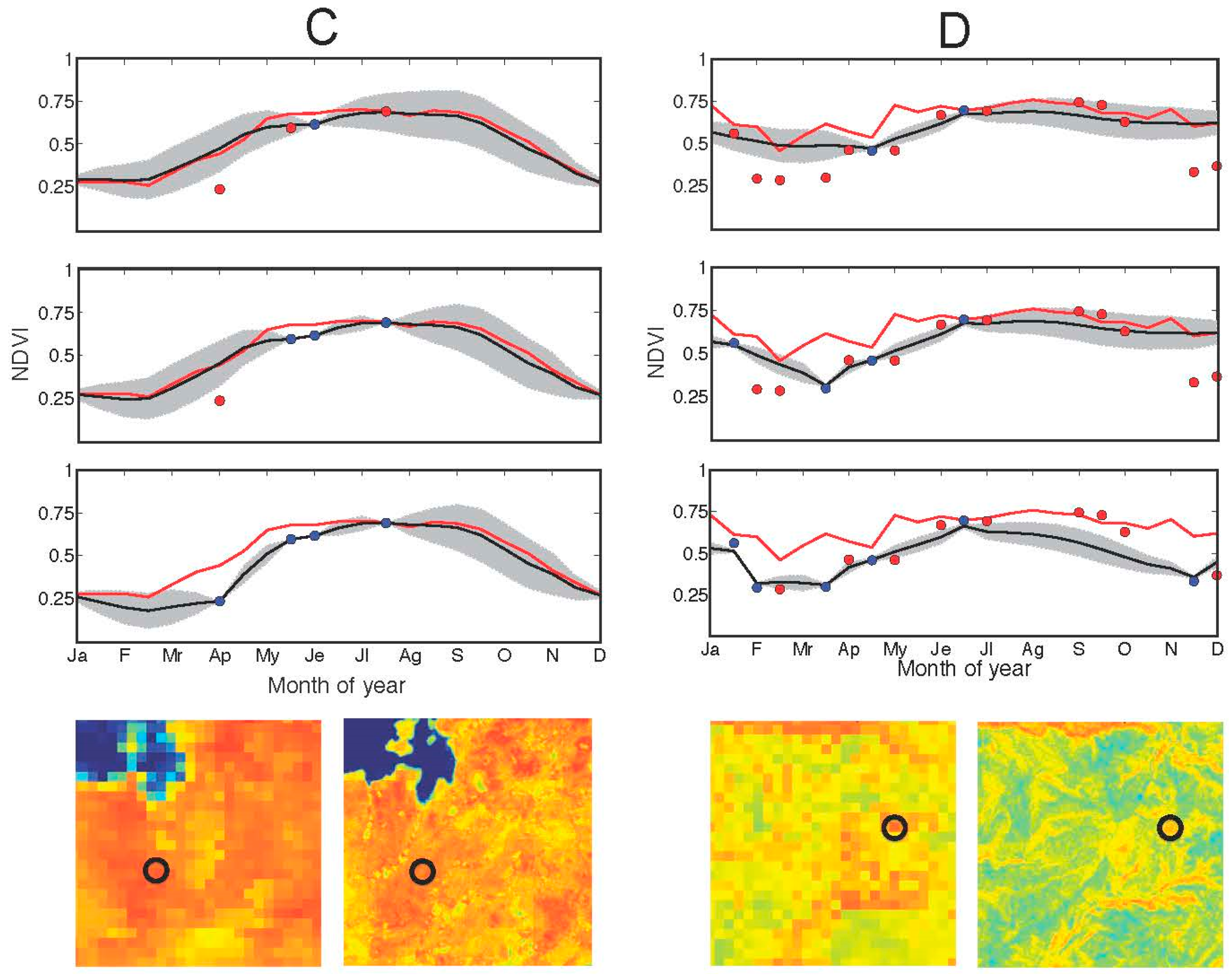
The time series of synthetic images in the four study sites captured the seasonal variations of NDVI values and revealed a more complex spatial structure than the NDVI MODIS time series. At the Kansas site, the KF-generated time series showed small fields with a clear border delineation, where the NDVI MODIS sequence only allowed the identification of large agriculture parcels and a fuzzy delineation of their limits. In this intensive agricultural landscape, the phenological pattern of the crops was discernible in both sequences, with NDVI values gradually increasing during the winter months to reach a maximum in the summer months and decline again towards autumn, with variations depending on the crop type and land use (
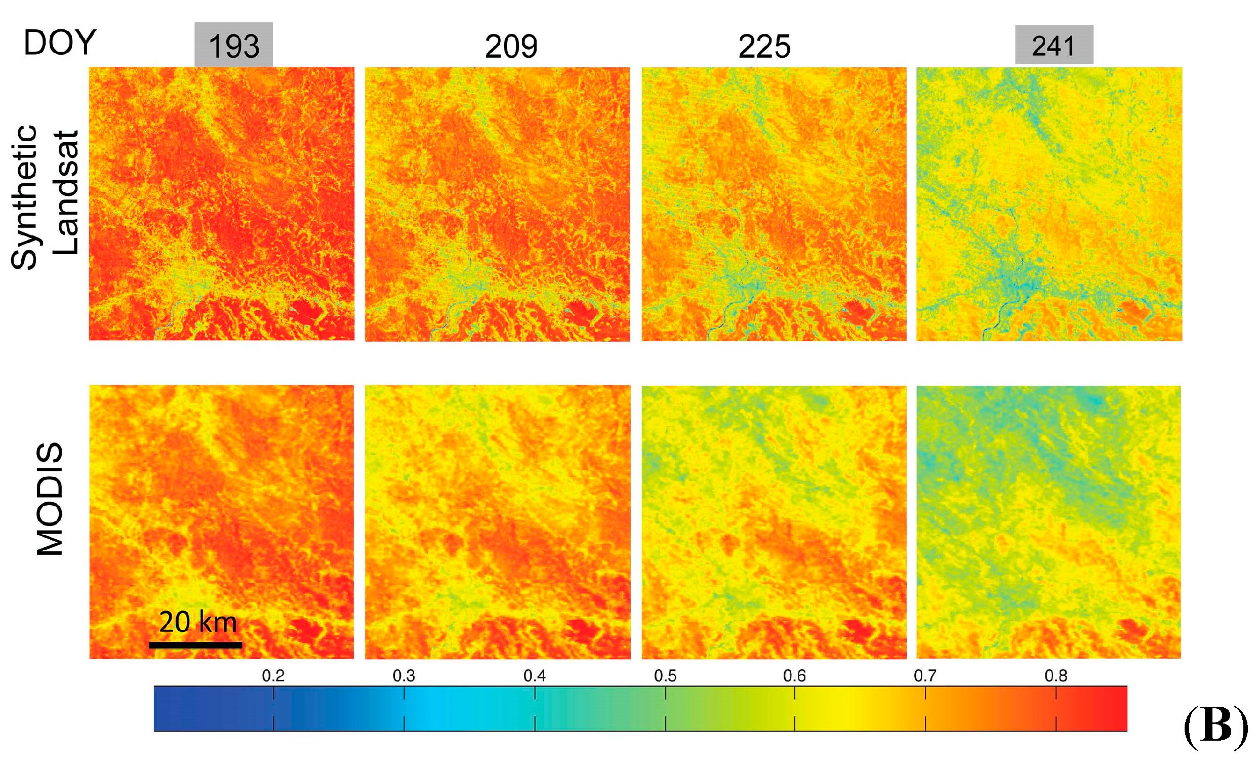
Figure 6a). At the Zambezia site, the NDVI MODIS images showed the main features of the surface within a landscape of quite homogeneous NDVI values. The synthetic time series revealed a more heterogeneous landscape with smaller features, such as subsistence agriculture openings, patches of dense and degraded forest and linear features, such as roads and rivers (
Figure 6b).
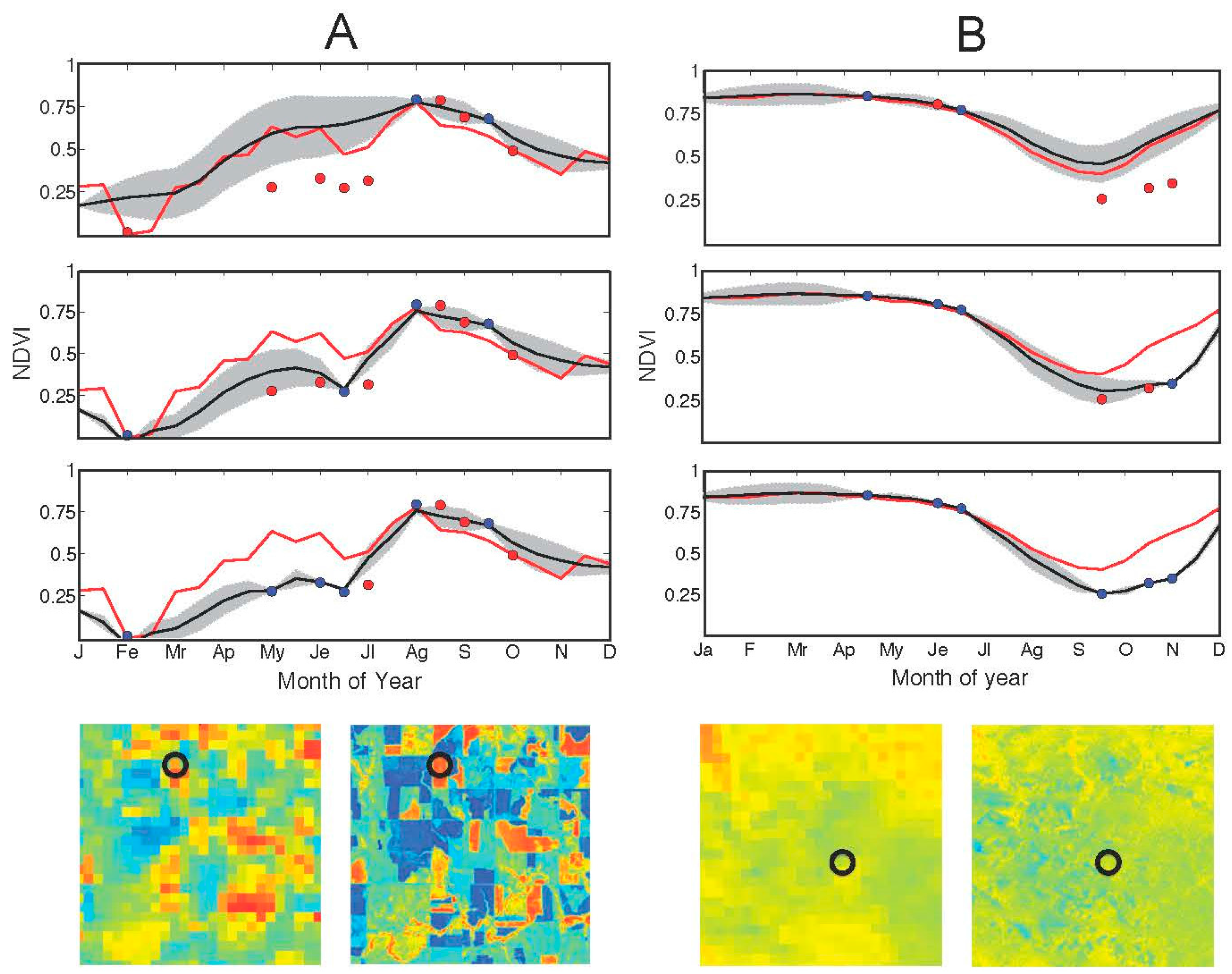
At the pixel level, time series of synthetic Landsat scenes kept the same general phenology trends of coarse-scale MODIS. However, while KF-generated NDVI time series created with few observations closely followed the NDVI MODIS temporal pattern, fine-scale differences in phenology emerge as the number of observations available to generate the sequence increased. The synthetic temporal sequence at the Kansas site showed lower NDVI values during spring months, with a faster rise reaching a peak in NDVI close to 0.75 in August, followed by a gradual decline (
Figure 7a). In Zambezia, both MODIS and the KF-generated curves captured the progressive decrease of NDVI values linked to the beginning of the dry season (July) and a later increase as rains trigger photosynthetic activity. The inclusion of more observation retrieved a slower NDVI recovery after the dry season (
Figure 7b). The NDVI temporal profiles of the Manitoba study site displayed an increase in NDVI values as spring advances, with a peak around 0.7 and a gradual decrease after September. The addition of observed data revealed that for some surfaces, the onset of the photosynthetic activity occurred later in the year, and the peak of annual NDVI values was reached more rapidly (
Figure 7c). In the case of the Arizona study site, despite the limited temporal variation in NDVI values, both the time series of synthetic images and the MODIS dataset show a drop in the late winter months associated with snow cover and a limited and gradual increase as the growing season advances. More NDVI Landsat observations in the calculation resulted in a profile with lower NDVI values and a significant drop in November’s values (
Figure 7d).
Figure 3.
MODIS, Landsat NDVI validation, synthetic NDVI images and spatially explicit residuals corresponding to one time step (k + 1) from the last Landsat observation for the 13 × 13-km subset of the site (A1–A5) and the 30 × 30-km subset of the Manitoba site (B1–B5). Prediction residual (A4 and B4) values are color coded: −0.05 ≤ purple, −0.05 < blue ≤ 0, 0 ≤ green < 0.2, 0.2 ≤ yellow < 0.4, 0.4 ≤ orange < 0.6, red ≥ 0.6. Plates A5 and B5 show residuals higher than ±0.25. (A) Zambezia site; (B) Arizona site.
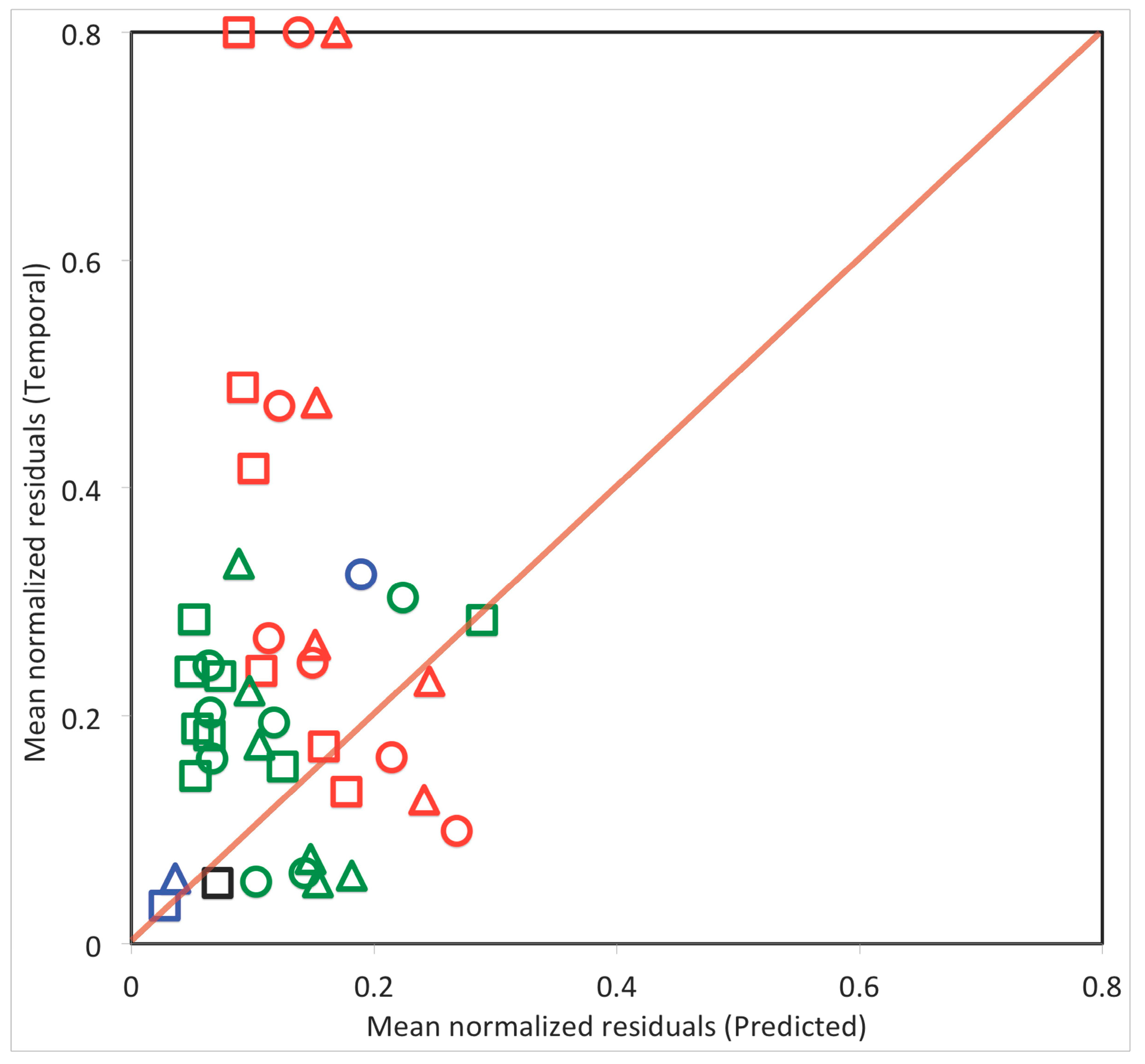
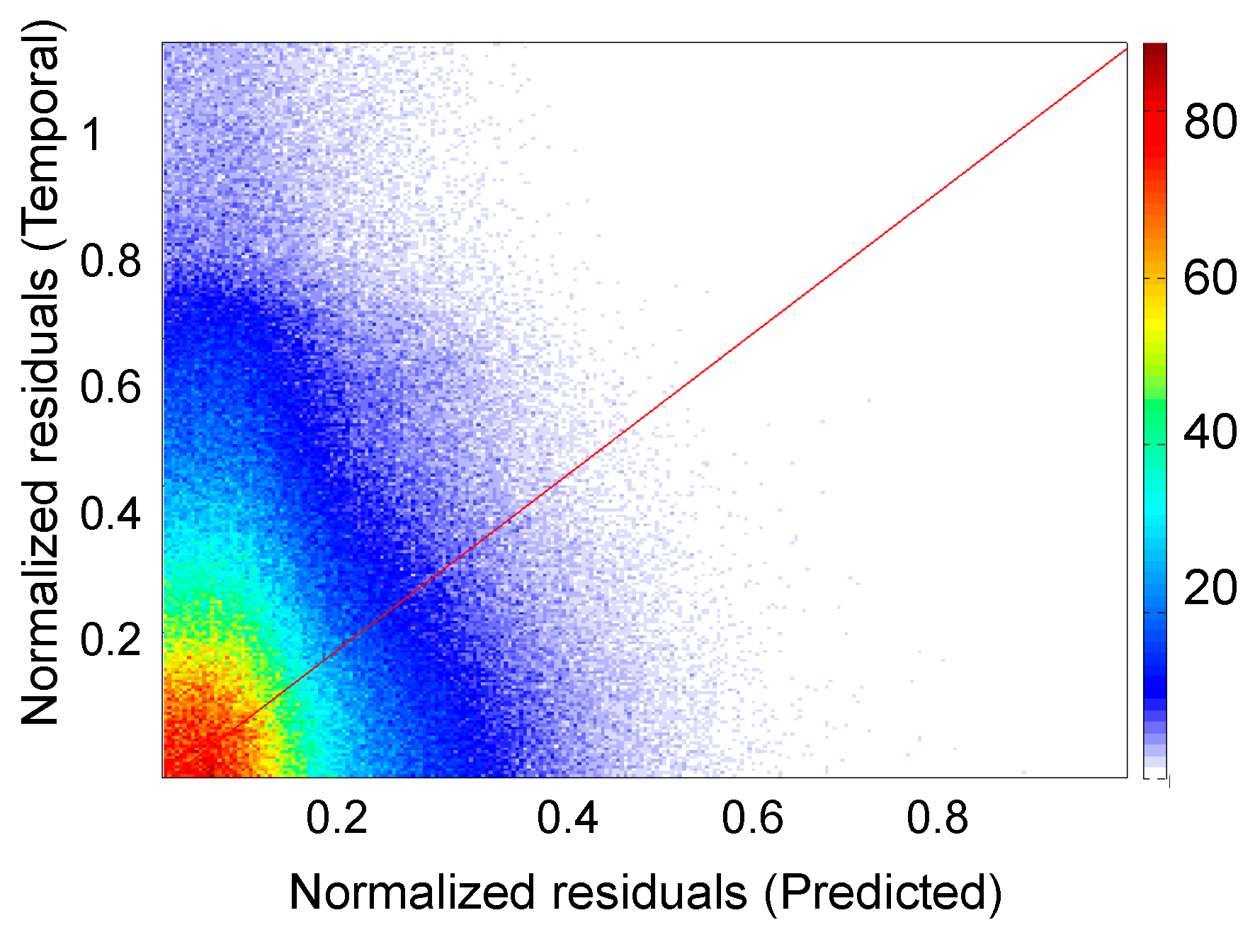
Figure 4.
Scatterplot of 67 image-level predicted and temporal mean normalized residuals for the four study sites: red (Kansas); blue (Mozambique); green (Arizona); black (Manitoba). Symbols indicate the number of time steps away of the synthetic image from the last Landsat observation: one time step observation, k + 1, (square); two time steps, k + 2, (triangle); three time steps, k + 3, (circle). Points with very high mean normalized values in the temporal axis indicate the presence of undetected clouds.
Figure 5.
Scatterplot of pixel-level predicted and temporal normalized residuals corresponding to one time step (k + 1) from the last Landsat observation for the Kansas site (k = DOY 160; k + 1 = 176). The larger number of points above the 1:1 line and the larger range of normalized temporal residuals values indicate that a reliable synthetic NDVI image has been generated. The normalized predicted residuals of 48% of the pixels in the image were below 0.1; 28% between 0.1 and 0.2; 13% between 0.2 and 0.3; 13% between 0.3 and 0.4; and 5% were higher than 0.4.
Figure 6.
(A) Time series of NDVI image subsets (9 km × 9 km) from the MODIS NDVI (MOD13Q1) and combined mode Kalman simulation NDVI images for the Kansas site. The time series includes eight 16-day periods starting in early May (DOY 120) and finishing in late August (DOY 241). The dates in grey indicate the time steps for which Landsat images were used as model observations. (B) Time series of NDVI image subsets (48 km × 48 km) from the MODIS NDVI (MOD13Q1) and combined mode Kalman simulation NDVI images for the Mozambique site. The time series includes four 16-day periods starting in June (DOY 193) and finishing in late September (DOY 241). The date in grey indicates the time steps for which a Landsat image was used as the model observation.
Figure 7.
NDVI pixel-level values for combined mode Kalman filter implementation time series for (A) Kansas, (B) Mozambique, (C) Manitoba and (D) Arizona for a variable number of Landsat images as model observations. The black line shows the NDVI time series retrieved from the Kalman filter implementation. The grey area indicates model uncertainties (±standard deviation from the model estimate). The red line shos the average seasonal NDVI pattern extracted from the MODIS NDVI 16-day composites (MOD13Q1). The blue dots indicate the time steps for which Landsat images where used as model observations. The red dots indicate the time steps for which Landsat images where not used as model observations. The images display snapshots of MODIS and synthetic Landsat images. The black circle in the NDVI snapshots indicates the location of the pixel shown in the time series.
For all four sites, mean residuals and mean normalized residuals of the time series of synthetic NDVI images decreased as the number of observations used to generate the temporal sequence increased. Residuals were also consistently lower for all sites in smoothing mode than in forward or backward filtering modes. The magnitude of the reduction in the residuals with the number of observations used to generate the temporal sequence varied from site to site (
Table 4,
Table 5,
Table 6 and
Table 7). In the case of the Kansas study site, the mean of normalized residuals for time series of synthetic NDVI images generated in combined mode with a single observation was 0.3, decreasing to 0.16 when three or more observations were included (
Table 4). For Zambezia, the mean normalized residuals for synthetic time series declined from 0.2 to 0.1 when one and five observations were used, respectively (
Table 5). At the Manitoba site, mean normalized residuals for synthetic time series generated in combined mode with one observation reached 0.32 and decreased to 0.16 when two observations were used (
Table 6). At the Arizona site, the decline was not as sharp in combined mode as in forward and backward modes. Mean normalized residuals for time series of synthetic NDVI images generated using only one observation reached 0.2 and gradually decreased to values of 0.16 when nine observations were included.
The average of the standard deviations of the residuals remained low and relatively stable for all sites as the number of observations increased (
Table 4,
Table 5,
Table 6 and
Table 7). The largest image-level normalized residual for a synthetic image within a temporal sequence decreased with the number of observations used to build the sequence. It also decreased when the algorithm was run in combined mode.
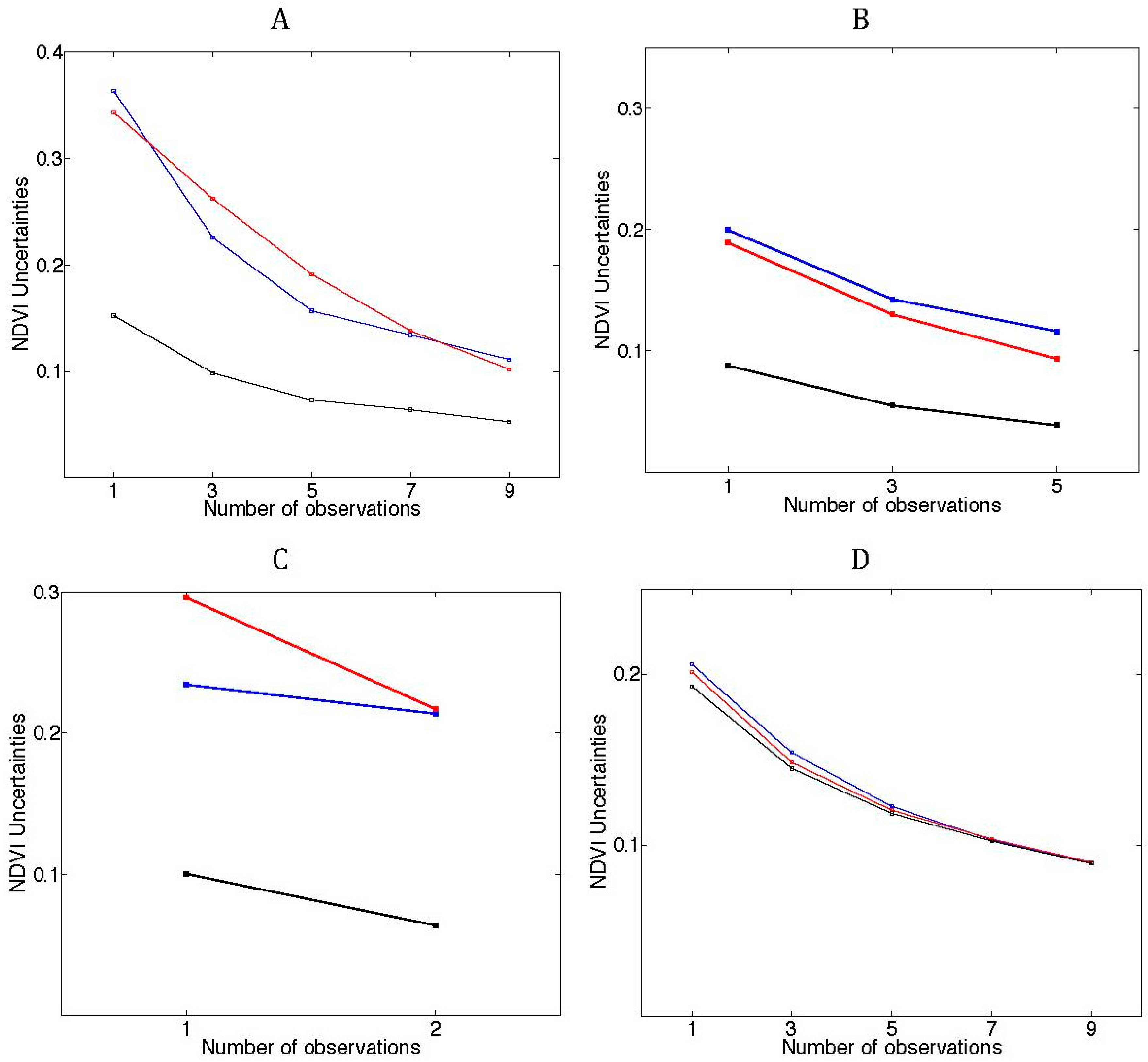
The model uncertainties also increased with time since the last observation, to be reduced in the event of a new Landsat scenes becoming available. A larger number of observations ensured shorter periods without observations and resulted in lower image uncertainties (
Figure 8). As a consequence, mean uncertainties decreased as more observations were used to produce the synthetic NDVI images. Combined mode synthetic images resulted in lower uncertainties than forward and backward modes (
Figure 8). At the Kansas site, mean uncertainties for the combined mode reached 0.15 for time series of synthetic NDVI images generated using only one observation and decreased under 0.05 when nine observations were used. In Zambezia, mean uncertainties declined from values close to 0.09 to 0.04 from one to five observation settings. For Manitoba, mean uncertainties moved from values close to 0.1 to 0.06 from one to two observation settings. At the Arizona site, the mean uncertainty for synthetic images in combined mode was 0.19 when a single observation was used and 0.09 when nine observations were used.
Table 4.
Kansas site. Summary statistics: temporal sequence level mean normalized residuals (mean), standard deviation (SD) and maximum image-level residuals (Max) calculated from all temporal sequences generated with the same number of Landsat observations in Monte Carlo simulations. Residuals are presented for forward, backward and combined mode recursions.
| Number Observations | Forward Mode | Backward Mode | Combined Mode |
|---|
| Mean | SD | Max | Mean | SD | Max | Mean | SD | Max |
|---|
| 1 | 0.306 | 0.04 | 0.438 | 0.315 | 0.04 | 0.442 | 0.141 | 0.01 | 0.195 |
| 3 | 0.229 | 0.05 | 0.438 | 0.246 | 0.04 | 0.411 | 0.103 | 0.02 | 0.190 |
| 5 | 0.177 | 0.04 | 0.420 | 0.195 | 0.04 | 0.391 | 0.081 | 0.01 | 0.171 |
| 7 | 0.144 | 0.04 | 0.395 | 0.163 | 0.05 | 0.374 | 0.068 | 0.01 | 0.156 |
| 9 | 0.130 | 0.06 | 0.233 | 0.161 | 0.09 | 0.323 | 0.067 | 0.03 | 0.106 |
Table 5.
Mozambique site. Summary statistics: temporal sequence level mean normalized residuals (mean), standard deviation (SD) and maximum image-level residuals (Max) calculated from all temporal sequences generated with the same number of Landsat observations in Monte Carlo simulations. Residuals are presented for forward, backward and combined mode recursions.
| Number Observations | Forward Mode | Backward Mode | Combined Mode |
|---|
| Mean | SD | Max | Mean | SD | Max | Mean | SD | Max |
|---|
| 1 | 0.200 | 0.03 | 0.328 | 0.189 | 0.02 | 0.308 | 0.088 | 0.01 | 0.126 |
| 3 | 0.143 | 0.04 | 0.237 | 0.130 | 0.04 | 0.259 | 0.055 | 0.02 | 0.108 |
| 5 | 0.116 | 0.07 | 0.210 | 0.094 | 0.06 | 0.184 | 0.039 | 0.02 | 0.068 |
Table 6.
Arizona site. Summary statistics: temporal sequence level mean normalized residuals (mean), standard deviation (SD) and maximum image-level residuals (Max) calculated from all temporal sequences generated with the same number of Landsat observations in Monte Carlo simulations. Residuals are presented for forward, backward and combined mode recursions.
| Number Observations | Forward Mode | Backward Mode | Combined Mode |
|---|
| Mean | SD | Max | Mean | SD | Max | Mean | SD | Max |
|---|
| 1 | 0.209 | 0.03 | 0.325 | 0.207 | 0.03 | 0.349 | 0.198 | 0.02 | 0.345 |
| 3 | 0.157 | 0.03 | 0.325 | 0.150 | 0.02 | 0.320 | 0.146 | 0.02 | 0.308 |
| 5 | 0.129 | 0.03 | 0.325 | 0.126 | 0.03 | 0.270 | 0.123 | 0.02 | 0.267 |
| 7 | 0.102 | 0.02 | 0.325 | 0.100 | 0.02 | 0.230 | 0.099 | 0.02 | 0.229 |
| 9 | 0.084 | 0.02 | 0.234 | 0.090 | 0.02 | 0.227 | 0.090 | 0.02 | 0.226 |
Table 7.
Manitoba site. Summary statistics: temporal sequence level mean normalized residuals (mean), standard deviation (SD) and maximum image-level residuals (Max) calculated from all temporal sequences generated with the same number of Landsat observations in Monte Carlo simulations. Residuals are presented for forward, backward and combined mode recursions.
| Number Observations | Forward Mode | Backward Mode | Combined Mode |
|---|
| Mean | SD | Max | Mean | SD | Max | Mean | SD | Max |
|---|
| 1 | 0.265 | 0.07 | 0.388 | 0.274 | 0.09 | 0.376 | 0.112 | 0.02 | 0.152 |
| 2 | 0.210 | 0.11 | 0.340 | 0.228 | 0.12 | 0.375 | 0.084 | 0.04 | 0.132 |
Figure 8.
Sensitivity of temporal level mean uncertainties to the number of observations (Landsat scenes) used to generate the temporal sequence: (A) Kansas; (B) Mozambique; (C) Manitoba; (D) Arizona. Temporal sequence level mean uncertainties were calculated from all temporal sequences generated with the same number of Landsat observations in Monte Carlo simulations. NDVI uncertainties are4 expressed as the standard deviation of the NDVI value for that state. Forward mode recursion (blue line); backward mode recursion (red line); combined mode recursion (black line).
5. Discussion
The performance of the method has been evaluated for various environmental settings and with input datasets of different qualities and numbers of observations. The quality of the outputs was consistent over the four study sites. The time series of synthetic images captured the seasonal variations of 250-m NDVI MODIS images, while retaining the spatial structure of NDVI Landsat images. The results showed that the residuals of the synthetic images retrieved by the method were in agreement with values reported in the literature for similar methods producing single synthetic images [
21,
37]. Average residuals for temporal sequences were also within the similar ranges of residuals (
Table 4,
Table 5,
Table 6 and
Table 7).
The inclusion of uncertainties in the calculation process provides a solid statistical framework, rather than single images, to produce full temporal sequences of synthetic images at given time intervals within a defined period. The uncertainties also enable the use of more general and simpler transition models in the implementation of this method. The unique seasonal trend for an entire site applied in this method to characterize seasonal vegetation patterns is a clear simplification of reality. More refined data-intensive and computationally-expensive alternatives to model land cover-based seasonal trends have been proposed in previous studies [
37,
42]. However, the results of our simulations show that the average normalized residuals for temporal sequences remained below 0.2, which indicates that accounting for uncertainties at each time step can compensate for the use of a simpler and more general transition model. A simpler transition model also adds generalization power to the method, ensuring that it can be used with limited medium-resolution observations of variable quality, in the absence of ancillary information and also remaining computationally efficient.
Since the uncertainties increase with the time lag from the last observation, the generation of reliable synthetic images relies on a sufficient and evenly-distributed number of observations (
Figure 7). In the absence of observations, the MODIS-based transition model dominates the Kalman filter algorithm, and the temporal profiles resemble those of the MODIS NDVI product (
Figure 7, top panels: A, B, C and D). As more observations are incorporated into the algorithm, the temporal profiles diverge from MODIS NDVI and distinct features emerge, reflecting the spatial heterogeneity at the MODIS subpixel scale (
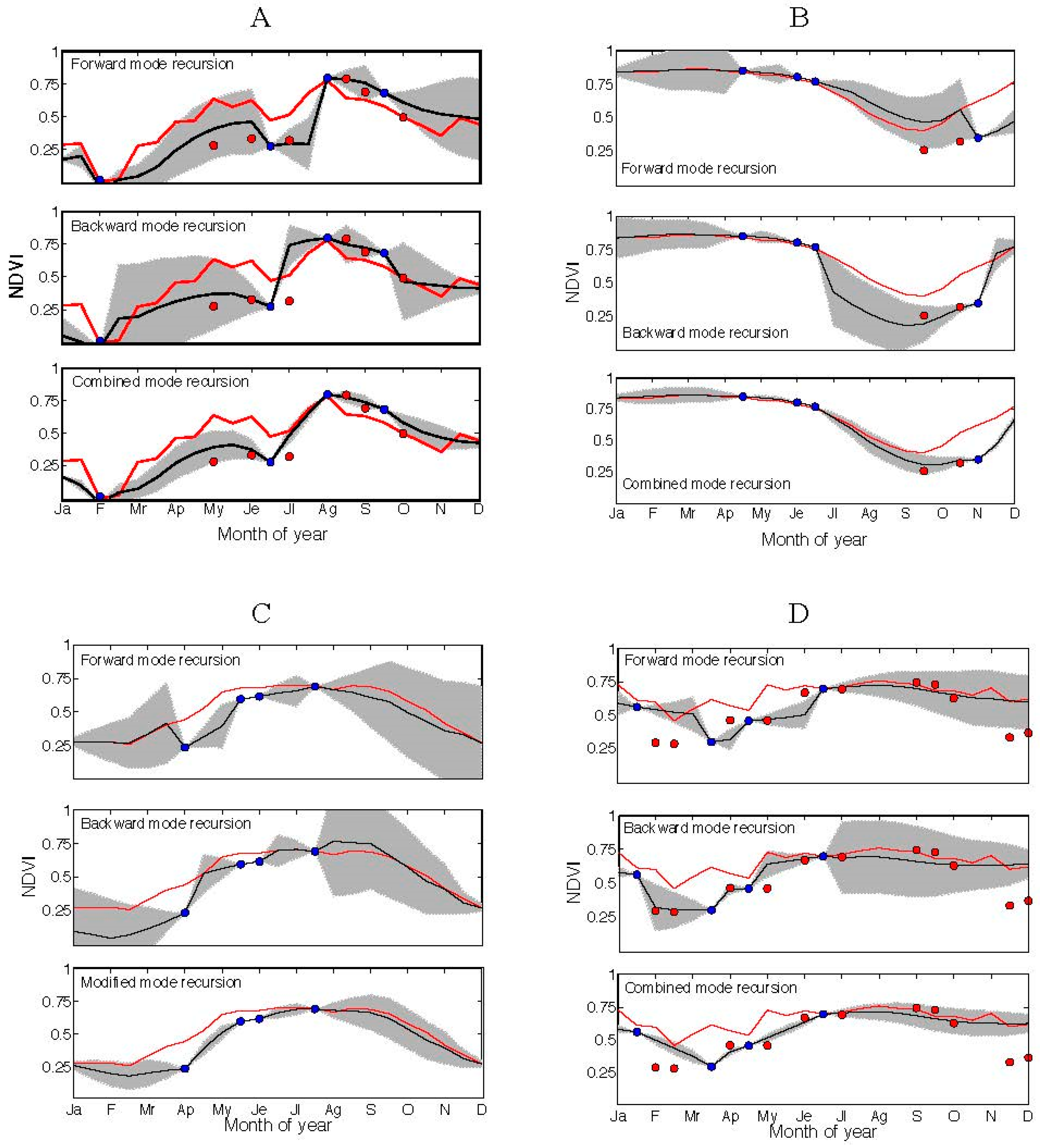
Figure 7). The results indicated that the number and distribution over time of the medium-resolution images used as observations by the algorithm are relevant in the detection of rapid land surface changes. Large numbers of evenly-spaced observations imply that synthetic images will be close in time to an actual observation. Under these circumstances, the probability of rapid small-scale changes occurring during that time span is lower. As a consequence, synthetic images and their closest observations are likely to be more similar, resulting in lower residuals and model uncertainties. As the number of observations decreases and/or they become unevenly distributed over time, some of the synthetic images in a temporal sequence are generated using medium-resolution information from further away time steps. As the time gap from the last available observation increases, surface changes, including rapid small-scale changes, are more likely to occur. If not captured by the MODIS imagery, these changes will not be retrieved in the synthetic image until a new observation is incorporated into the sequence, resulting in higher residuals and uncertainties of the synthetic images. The implementation of the forward and backward modes consecutively in a combined mode reduces the time gap between synthetic images and the last available Landsat observation, resulting in lower uncertainties of the synthetic images and improving the capacity of the method to detect rapid small-scale land cover changes (
Figure 9).
The method requires an adequate co-registration of moderate and medium-resolution images, a cloud and cloud shadow mask and preferably atmospherically-corrected data. The introduction of abnormal pixel values due to any of the above-mentioned causes could result in erroneous estimates and higher uncertainties that would propagate to subsequent states. Equally, the wavelength or the variable for which the sequence of synthetic images is generated must be available from both the moderate and the medium-resolution sensors. The existence of complete time series of moderate spatial resolution observations within the period of study and at least one medium-resolution observation within that period is also a requirement for the implementation of the method.
The scale difference between the moderate- and medium-resolution imagery is a potential source of limitations for the generation of reliable time series of synthetic images. The seasonal patterns generated from the moderate-resolution imagery within the KF algorithm will not capture the specific and distinct seasonal trends of subpixel land surfaces. The impact can be particularly distinct in areas of intense land use management with very different spectral signatures from their surroundings, such as small parcels of irrigated agriculture. The effect will be also evident when medium-resolution observations are scarce and far in time from the periods in which major land surface changes occur. While the scale difference between the 250-m MODIS NDVI product and the 30-m Landsat NDVI used in this study is not extreme, this impact would increase for the generation of synthetic images relying on coarser spatial resolution products.
The method does not explicitly account for viewing and illumination angles. Instead, a submodel is introduced to implicitly account for potential non-linearities between concurrent moderate- and medium-resolution images. Anisotropic properties from land surfaces affect spectral reflectance, vegetation indices and other remote sensing-based biophysical variables. These effects are particularly relevant in moderate resolution sensors with a large field of view [
69], such as MODIS. This study uses MODIS NDVI from MOD13Q1, which uses a simple BRDF model [
51] and an angular compositing method to minimize angle effects and BRDF-related issues. The MODIS nadir BRDF-adjusted reflectance product (MCD43A4) provides 16-day composites at 500-m spatial resolution, and it is a potential alternative dataset to minimize these effects [
38]. However, for this study, the higher spatial resolution of MOD13Q1 was preferred to keep a lower scale difference between the moderate- and medium-resolution imagery. Medium-resolution sensors, with a narrow field of view, are not severely affected by view angle variation, but solar illumination variations remain when acquisitions span a full year [
21,
70,
71]. Although some methods to correct these effects have been proposed in the literature [
32,
70], their implementation is not always feasible. Therefore, the Landsat imagery was not radiometrically normalized in this study.
As the Landsat archive expands and more fine-resolution Earth observation sensors (Disaster Monitoring Constellation, IRS-LISS III, SPOT, Sentinel 2,
etc.) become available, the analysis of land surface dynamics and ecosystem processes enters a new era of increasing possibilities for Earth system monitoring [
44]. While this study used MODIS and Landsat as sources of moderate- and medium-resolution data, other sensors can potentially be used as input for the proposed method. Future work will test the integration of medium-resolution imagery from several instruments. Moreover, following a similar approach, the method can be adapted to produce sequences of synthetic images for other ecosystem variables, provided that they can be calculated from both moderate- and medium-resolution resolution instruments. Examples include additional vegetation indices, leaf area index [
72], fraction of photosynthetically active radiation [
73,
74,
75,
76], albedo [
77], net primary productivity, snow, water and burn indices,
etc.
Figure 9.
NDVI pixel values for combined mode Kalman filter implementation time series for (A) Kansas, (B) Mozambique, (C) Manitoba and (D) Arizona for forward, backward and combined recursive modes. The black line shows the NDVI time series retrieved from the Kalman filter implementation. The grey area indicates model uncertainties (±standard deviation from model estimate). The red line shows the average seasonal NDVI pattern extracted from the MODIS NDVI 16-day composites (MOD13Q1). The blue dots indicate the time steps for which Landsat images where used as model observations. The blue dots indicate the time steps for which Landsat images were used as model observations.
This approach is pixel-based, does not require parameter tuning and can be implemented independently of the number of existing medium-resolution images. Its robustness and flexibility make it potentially suitable for large-scale operational applications. The retrieval of complete time series at a higher spatial resolution enables the extraction of seasonal metrics and spectral libraries for operational vegetation mapping [
78,
79]. Equally, the time series of synthetic medium-resolution data can potentially contribute to filling the gaps of large-scale medium-resolution mosaics, such as the Web-enabled Landsat Data (WELD) [
33]. The development of methods for continuous monitoring of land surfaces at medium spatial resolution will, in the coming years, improve our capabilities for continuous monitoring of land surfaces.


